Improving Remote Species Identification through Efficient Training Data Collection

Abstract

Plant species identification and mapping based on remotely-sensed spectral signatures is a challenging task with the potential to contribute enormously to ecological studies. Success in this task rests upon the appropriate collection and use of costly field-based training data, and researchers are in need of ways to improve collection efficiency based on quantitative evidence. Using imaging spectrometer data collected by the Carnegie Airborne Observatory for hundreds of field-identified tree crowns in Kruger National Park, South Africa, we developed woody plant species classification models and evaluated how classification accuracy increases with increasing numbers of training crowns. First, we show that classification accuracy must be estimated while respecting the crown as the basic unit of data; otherwise, accuracy will be overestimated and the amount of training data needed to perform successful classification will be underestimated. We found that classification accuracy and the number of training crowns needed to perform successful classification varied depending on the number and spectral separability of species in the model. We also used a modified Michaelis-Menten function to describe the empirical relationship between training crowns and model accuracy, and show how this function may be useful for predicting accuracy. This framework can assist researchers in designing field campaigns to maximize the efficiency of field data collection, and thus the amount of biodiversity information gained from remote species identification models.

1. Introduction

Identification and mapping of woody plant species from remotely-sensed imagery is an emerging field of research with great potential to contribute to ecology and ecosystem management. Several studies have examined the potential for tree species identification based on species’ spectral signatures [1–8]. Thus far, successful application of remote species identification models has been accomplished for only a handful of study ecosystems, usually of low to moderate diversity. For example, classification models have been successfully applied for the remote species identification of individual tree crowns in boreal forests [9], temperate montane forest [10], mixed open forest [11], semi-arid savanna [12] and Hawaiian tropical forest [13]. While the results from these studies are encouraging, the full potential of remote sensing technology to map species distributions in most ecosystems remains poorly understood.

Many advances supporting remote species classification have come from improvements to spectral sensors, increasing the spatial and spectral resolution of images and the signal-to-noise ratio of spectra, as well as exploration of different classifiers and classification techniques. An equally important step in the process is the gathering of suitable training data, as the quality of a classification model critically depends on the quantity and distribution of training data across the different model classes [14]. Here, we refer to the “quality” of a classification model as including both the accuracy of the model and the number of species that are included (the “scope” of the model). At the same time, acquisition of training data is very labor and cost intensive. This step may not present much difficulty in ecosystems with few species, but may become quite difficult in diverse ecosystems when it is desirable to map many species. Therefore, we need ways to make the most of costly field work; specifically, to optimize the accuracy and scope of classification models given a finite amount of resources devoted to the collection of training data.

Classification accuracy has been shown to be positively related to the amount of training data across different types of classifiers and remote sensing classification tasks, e.g., [15,16]. In a remote species identification task, Féret and Asner [13] found accuracy increasing non-linearly with greater amounts of training data, showing sharp increases at first but with the gain in accuracy decreasing as the accuracy approaches an asymptote. The shape of this curve indicates that there is some optimal amount of training data to collect: that one should collect until the gain in model accuracy no longer justifies the cost. In practice, training data may be collected in a manner which randomly samples the vegetation of a landscape, creating an uneven distribution of training data among the potential model classes (species). Thus, some species may be greatly oversampled, while others may be severely undersampled. Knowledge of when this “optimal” point is reached would be useful during field campaigns for optimizing the distribution of training data among the desired model classes.

However, previous analyses of the relationship between species classification accuracy and the amount of training data have been performed at the pixel level, meaning that pixels were randomly drawn from the full set of labeled data for each class and added to the training set. This method ignores the inherently nested structure of the training data used in species classification tasks, in which pixels are non-independent spectral measurements that are grouped into tree crowns. We would expect greater similarity of spectral measurements taken from the same crown compared to measurements from different crowns of the same species due to genetic and environmental effects on vegetative traits, and this is supported by evidence from studies of the variation in leaf chemical, structural, and spectral properties, e.g., [8,17,18]. This is also expected because of spatially structured variation in reflectance across an image due to differences in illumination and viewing angle. When spectral differences exist among crowns, then classification accuracies that are evaluated at the pixel level—with pixels randomly assigned to training and test datasets regardless of crown membership—may provide unrealistic accuracy estimates. Specifically, the accuracy evaluated in this way may not reflect the accuracy obtained when applying the model to new crowns. This effect could also have important implications for the nature of the observed relationship between the quantity of training data and classification accuracy.

Other factors expected to influence accuracy estimates are the number of species to be classified and the spectral separability of those species. The number of species in a model is known to affect classification accuracy, with more species leading to lower accuracy [13]. We would also expect that the spectral separability of species would affect classification accuracy, with more spectrally distinct species being classified with greater accuracy. Less apparent, however, is whether these factors also influence the shape of the relationship between the quantity of training data and classification accuracy. Changes in the shape of this relationship—either apparent changes due to the treatment of the data or real changes due to the inherent difficulty of the classification task—could affect an assessment of the amount of training data that must be collected for successful classification.

We used imaging spectrometer data collected by the Carnegie Airborne Observatory (CAO) over an African savanna and hundreds of field-identified tree crowns to investigate how classification accuracy increases with greater amounts of training data. We explored how this relationship was affected by the treatment of pixels as independent spectral measurements. We also examined how the number of species included in the model and the spectral separability of those species influenced the accuracy relationship and the amount of training data needed to obtain good classification results. The understanding of these relationships gained from this study and others lead us to propose a framework for how to best evaluate model accuracy and help researchers plan efficient field data collection campaigns, supporting the construction of models with both greater accuracy and greater species modeling capacity.

2. Methods

2.1. Spectral Data

The landscape of Kruger National Park (KNP; Figure 1), South Africa, is a classic savanna landscape, consisting of a spatially patchy mixture of woody and herbaceous vegetation. The topography is relatively flat and characterized by shallow undulating hills. The mean annual temperature is approximately 22 °C and the mean annual precipitation is approximately 550 mm/yr. Many of the common tree and shrub species belong to the genera Acacia and Combretum. More information about the landscapes of KNP can be found in [19].

The Carnegie Airborne Observatory (CAO) Alpha system [20] was flown over several areas of KNP in April–May 2008. All images were collected between 9:00 am and 1:00 pm, local time. The CAO Alpha system combines three instrument subsystems into a single airborne package: (i) a High-fidelity Imaging Spectrometer (HiFIS); (ii) a Light Detection and Ranging (LiDAR) scanner; and (iii) a Global Positioning System-Inertial Measurement Unit (GPS-IMU). The CAO HiFIS subsystem provided spectroscopic images spanning the visible-near infrared spectral range between 384.8 and 1054.3 nm, resampled to 9.4 nm spectral resolution. The HiFIS is a pushbroom imaging array with 1500 cross-track pixels, and was flown at an altitude of 2 km providing 1.12 m pixel resolution. The LiDAR subsystem was operated in discrete-return mode, with up to four returns per laser shot. Laser beam divergence was designed to match the field-of-view of the imaging spectrometer for accurate alignment of spectroscopic and laser return data [20]. The GPS-IMU subsystem provided three-dimensional positioning and attitude data for the CAO-Alpha system for accurate projection of HiFIS and LiDAR data onto the land surface.

Radiance data from the imaging spectrometer were converted to surface reflectance using ACORN 5BatchLi (Imspec LLC, Palmdale, CA, USA) with a MODTRAN look-up table to compensate for Rayleigh scattering and aerosol optical thickness. The reflectance data were adjusted using a kernel-based bidirectional reflectance distribution function model to correct for cross-track reflectance gradients [3]. Lastly, the vegetation height information provided by the LiDAR subsystem was used for the accurate orthorectification of the spectral data [20]. A sample of the CAO imagery is displayed in Figure 1b.

Within the overflight areas, over one thousand individual tree and shrub crowns were identified to species and their location was recorded using a survey-grade handheld Global Positioning System (GPS) with differential correction during post-processing (GS50 Leica Geosystems Inc., Norcross, GA, USA). These crowns were manually delineated within the images and their corresponding pixels were extracted to construct a library of species’ spectral signatures. Prior to analysis, noisier spectral bands at the lower and upper portions of the spectra were eliminated, for a total of 54 bands spanning 517 nm to 1016 nm. Additionally, the crown spectral data were filtered to contain only well-lit, leafy vegetation pixels with NDVI ≥ 0.5 (NIR band = 857 nm, VIS band = 649 nm) and mean NIR (850–1016 nm) reflectance ≥ 20%, and crowns occupying at least three such pixels. For our analysis, we used crowns from 11 species having at least 30 crowns each: Acacia nigrescens, Acacia tortilis, Combretum apiculatum, Combretum hereoense, Combretum imberbe, Colophospermum mopane, Diospyros mespiliformis, Euclea divinorum, Philenoptera violacea, Sclerocarya birrea, and Terminalia sericea. These crowns had an average of 24.9 pixels per crown.

2.2. The Relationship between the Number of Training Crowns and Model Accuracy

We used the support vector machine (SVM) as the classifier for this analysis. SVM is a non-parametric classifier which is widely used in the remote sensing community due to its excellent performance in classifying unknown samples based on relatively small amounts of training data [21–23]. Additionally, SVM showed good performance in a previous species mapping task with this particular dataset [3,12]. SVM performs an implicit mapping of the data into a higher dimensional feature space through the application of a kernel function. We used a radial basis function kernel, requiring the fitting of two parameters for the SVM: λ, which controls the width of the kernel function, and C, which controls the penalty associated with classification error. Optimal values of these parameters were found through an exhaustive grid search, with each combination evaluated via four-fold cross validation. SVMs were constructed using the “e1071” package [24] of the R programming language [25].

We evaluated a series of classification models to characterize the relationship between the number of crowns used to train the model and classification accuracy. We varied the number of training crowns per species (n) from one to 25. For each value of n, n crowns were selected from each of the 11 species to form the training data and five separate crowns were selected from each species to form the test data. The overall accuracy was recorded as the percent of pixels in the test dataset that were correctly classified. This process was repeated 100 times for each value of n, producing a curve of the classification accuracy in relation to the number of crowns used to train the classification model. We note that although we treat the crown as the basic unit of data for training a model (representing what is collected in the field), we were primarily interested in assessing model accuracy at the pixel level.

2.3. Variation Partitioning and the Relevance of Among-Crown Variation

To explore how spectral measurements vary among crowns of the same species, we partitioned the total spectral variation of each species into within-crown and among-crown components. For each species, the total variation was partitioned with a nested, random-effects MANOVA, with pixels nested within crowns, which quantifies the proportion of the total variation explained by crown identity. Because the reflectances of the spectral bands are highly intercorrelated, the Mahalanobis distances between individual spectra (pixels) were used rather than Euclidian distances. The Mahalanobis distances were determined by the species’ spectral covariance matrices, accounting for the hyper-ellipsoidal shape of each species in spectral space.

The presence of among-crown variation indicates that the pixels contained in a crown represent a non-independent spectral sample of a species. To evaluate the relevance of this among-crown variation to the observed relationship between the amount of training data and model accuracy, we re-constructed this relationship while violating the boundaries defined by crown units. This was done in two ways: In the first variant, five test crowns from each species were set aside to form the test data as in the previous analysis. Then, the training data were created by randomly drawing pixels from the remaining crowns of each species. This was done so that the number of pixels used in each model matched the number of pixels used in a corresponding model of the previous analysis (Section 2.2). In the second variant, both the training and test pixels were drawn randomly from the entire pool of pixels available for a species, while keeping the number of training and test pixels equal to the numbers used in the previous models.

2.4. Fitting the Relationship

We found that the accuracy curves were well-fit by a scaled, shifted Michaelis-Menten function. This is a simple and intuitive function, allowing for straightforward inferences about the relationship given the fitted values of the parameters [26]. The function is given by the formula

$$y=\frac{a(x-c)}{b+x-c}+d$$

(1)

where x is the number of training crowns, y is the classification model accuracy, and a, b, c, and d are the fitted parameters. The parameter c is the lower bound of the function on the x axis, which was set to one in all cases (the lowest number of crowns per species that could be used to train the model was one). The parameter d is the lower bound of the function on the y axis, or the classification accuracy at one training crown per species. The parameter a is the maximum additional accuracy that can be gained by adding more training data, and thus the asymptote of the relationship is given by a + d. This function was fit to the accuracy curves by finding the maximum likelihood estimates of the parameters a, b, and d.

2.5. Species Number and Spectral Dissimilarity

We also investigated how the number of species in a model and their spectral similarity would affect classification accuracy as well as the number of crowns needed to construct a satisfactory model. By this, we mean that the accuracy has reached a point that is close to the asymptote, but the additional accuracy that would be gained by adding more training data has fallen to a point where it no longer justifies the cost. Locating this point on the curve requires a value judgment by the researcher, but for the purposes of comparison across many accuracy curves, we defined this to be the smallest value of n for which increasing n by one would increase the model accuracy by less than 0.5% (we call this C_0.5%). We repeated the analysis of model accuracy with respect to the number of training crowns (Section 2.2) for different numbers of species. The 11 species in our dataset yielded 55 unique pairwise species combinations, and we repeated the accuracy analysis for each of them. To create models with more species, either five or eight species were selected at random from the pool of 11 species, and the accuracy analysis was performed on this set of species. This was repeated 55 times for each number of species, for a total of 55 unique combinations of two, five, and eight species, along with the single 11 species model.

The radial basis function parameters γ and C were optimized separately for each accuracy analysis (each distinct set of species) using 25 crowns from each species. These values of γ and C were used for all models containing that same set of species. The modified Michaelis-Menten function (Section 2.4) was fit to each accuracy curve, and properties of the fitted curves, including the asymptote and C_0.5%, were derived from the fitted curves. All fitted curves were visually inspected to ensure the quality of the values obtained.

We also expected that the accuracy of a classification model and the number of crowns needed to obtain good classification results would be related to the spectral separability among the species in the model. We quantified the spectral separability between species for all 55 pairwise species combinations using the Bhattacharyya distance [27,28]. This metric quantifies the integrated difference between two species over the full spectral range, and has performed favorably in recognizing differences between species compared to other spectral separability metrics [13]. The Bhattacharyya distance is given by the formula.

$$\mathit{Bhattacharyya} \mathit{distance}=\frac{1}{8}{\left({\mu }_i-{\mu }_j\right)}^T{\sum }^{-1}\left({\mu }_i-{\mu }_j\right)+\frac{1}{2}\text{ln}\left(\frac{|\sum |}{\sqrt{\left|{\sum }_i\right|\left|{\sum }_j\right|}}\right)$$

(2)

where μ_i and μ_j are the mean values across all spectral bands for species i and j, ∑_i and ∑_j are the covariance matrices for each species, and ∑ is the pooled covariance matrix. We then tested whether the spectral dissimilarity between two species was related to the fitted accuracy at n = 25 training crowns (A₂₅) and C_0.5% of the accuracy relationship for classifications differentiating those species. The relationship between the pairwise Bhattacharyya distance and A₂₅ and C_0.5% were evaluated using Mantel tests, with significance determined by 9999 random permutations of the matrices.

2.6. Predicting the Relationship between Training Data and Accuracy

To explore the possibility of predicting the accuracy curve given only a subset of crowns, we subsetted the full crown dataset and predicted the accuracy curve beyond what could be directly assessed with the subset. We created the subset randomly sampling 10 crowns per species. Then we repeated the procedure for performing the accuracy analysis (Section 2.2), except in this procedure, n ranged from one to nine crowns, and one crown per species was used to evaluate accuracy. Using the accuracy values generated by the 100 repetitions at each of the nine levels of n, we generated bootstrapped 95% confidence intervals for the fitted accuracy curve up to 25 crowns. This was done by resampling the data 1000 times, fitting the modified Michaelis-Menten function to each bootstrapped sample, and generating the 95% quantiles of the fitted relationship from one to 25. Thus for a given subset of 110 crowns, we generated a 95% confidence envelope for the fitted accuracy relationship that extended up to 25 crowns. We repeated the subsetting and bootstrapping procedure 100 times, creating 100 confidence envelopes for the true relationship. We then evaluated how well our predictions created from the crown subsets performed in predicting the true relationship by recording how many times the true relationship fell within the confidence envelopes.

3. Results

The full 11 species classification model showed the expected non-linear relationship between the number of input training crowns and the accuracy assessed on an independent set of crowns (Figure 2a). The accuracy increased from an average of 30.1% for models trained with only one crown per species to an average of 74.3% accuracy for models trained with 25 crowns per species. By fitting the modified Michaelis-Menten function to the relationship, we estimated that the asymptote for this relationship was 82.7% accuracy and the number of crowns per species needed to obtain good accuracy (C_0.5%) was 19 crowns. There was excellent fit between the observed data and the modified Michaelis-Menten function (Figure 2b), and similar fit was observed for all accuracy curves generated in this study.

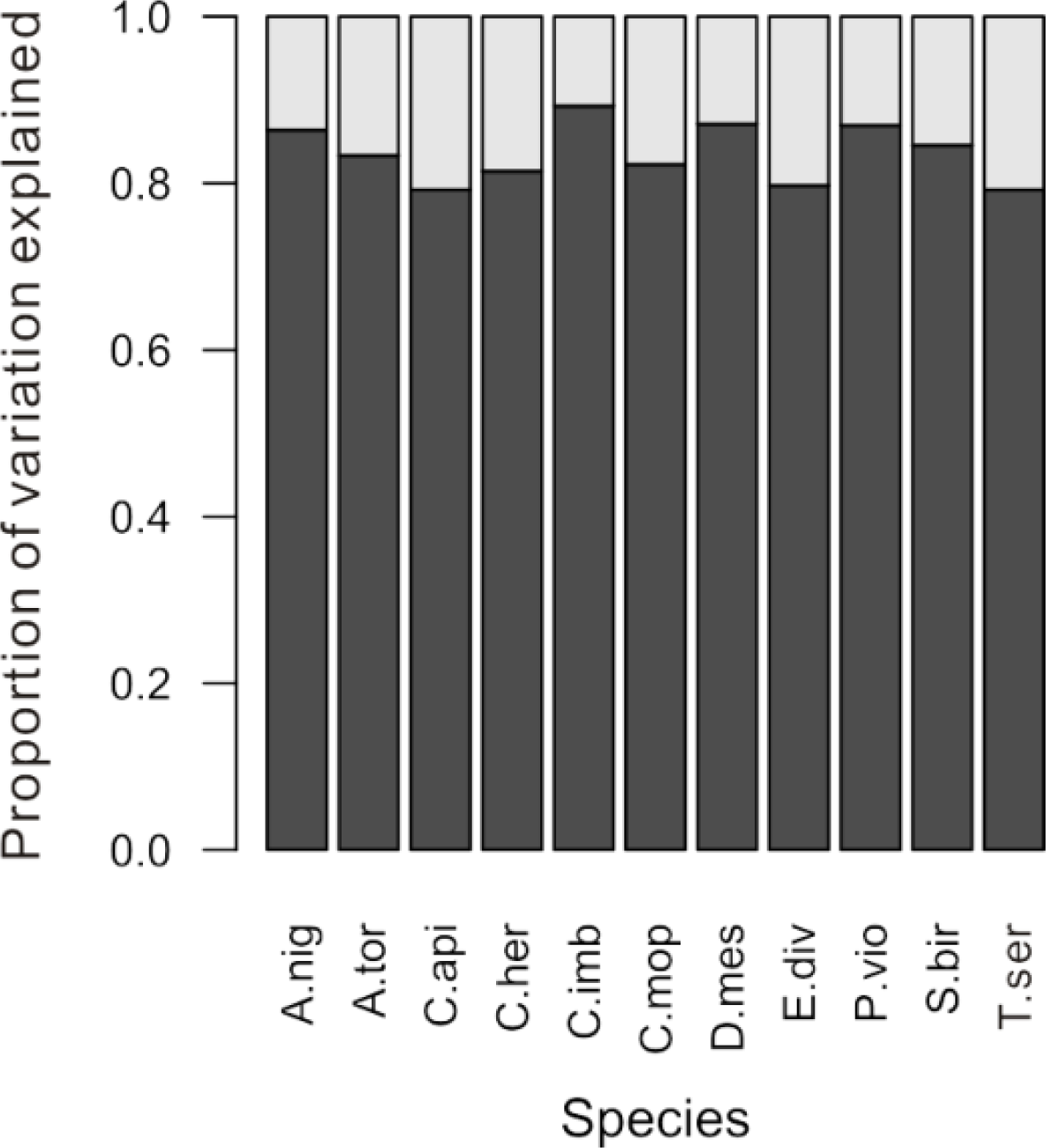
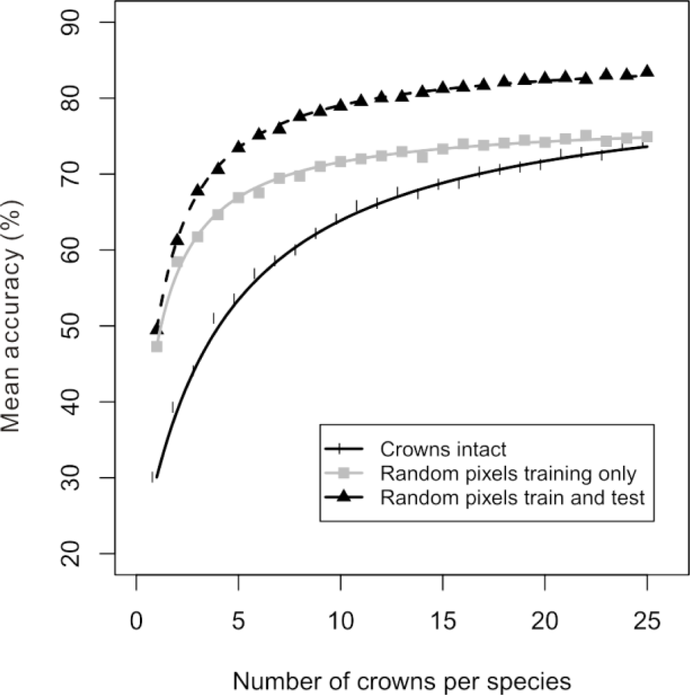
From the variation partitioning analysis, we found that 11%–21% of the spectral variation within a species was explained by crown identity (representing among-crown variation), while the remaining 79%–89% of the variation was unexplained (representing within-crown variation) (Figure 3). Although spectral variation among crowns accounted for a relatively small portion of the overall variation within a species, it was enough to cause substantial differences between accuracy estimates that were generated in different ways. Compared to the previous method of randomly selecting intact crowns to create the training dataset (black line in Figure 4), the accuracy evaluated on a separate set of testing crowns increased when training pixels were randomly drawn from the set of training crowns (gray line in Figure 4). The increase in the estimated accuracy was present across all amounts of training data, but was greatest for smaller amounts of training data, with the two accuracy curves reaching similar accuracy estimates for large amounts of training data. From this curve, the C_0.5% was calculated as the pixel equivalent of 10 crowns per species. When training pixels and test pixels were both randomly drawn from the pool of all pixels for a given species, the estimated accuracy was even higher (dashed line in Figure 4). This increase in estimated accuracy was substantial regardless of the amount of training data—always more than 9% but sometimes as great as 22%. From this curve, the C_0.5% was calculated as the pixel equivalent of 11 crowns per species.

The properties of the accuracy curve were also found to be influenced by the number of species included in the model and the spectral separability among species. As the number of species included in the classification increased, accuracy decreased for all amounts of training data (Figure 5a). The asymptotic accuracy of these relationships decreased from an average of 96.9% for two species classifications to 82.7% for the full 11 species classification (Figure 5b). 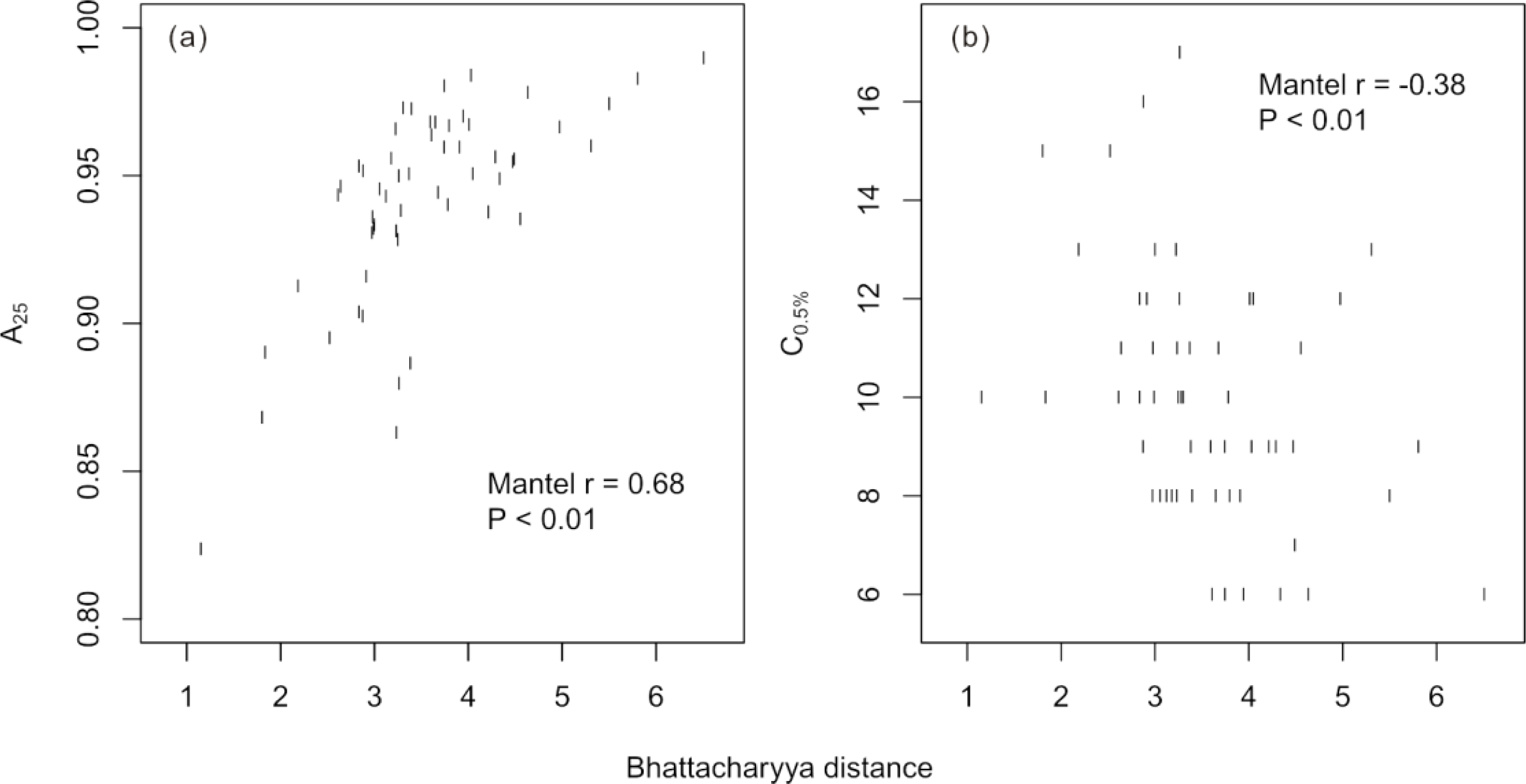The C_0.5% increased with more species included in the classification, from a mean of approximately 10 crowns for two species classifications compared to the 19 crowns needed for the 11 species classification (Figure 5c). Over all possible two-species models, the Bhattacharyya distance between species was positively related to the model accuracy evaluated at 25 training crowns (Mantel r = 0.68, p < 0.01) and negatively related to the C_0.5% of the accuracy curves (Mantel r = −0.38, p < 0.01; Figure 6).

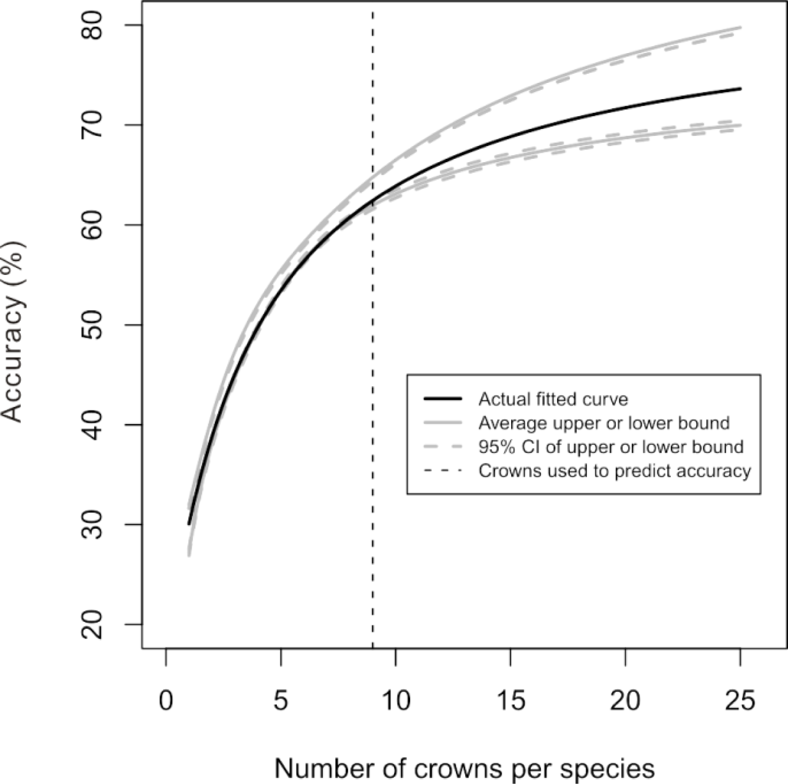
In the simulations where an initial dataset was used to predict the accuracy relationship for greater numbers of crowns, we found that all of the simulated datasets with only 10 crowns per species generated confidence intervals that encompassed the relationship generated with all available data (Figure 7). The 95% confidence envelope for the predicted relationship widened as the accuracy was predicted for greater numbers of crowns, reflecting greater uncertainty in the prediction.

4. Discussion

We took advantage of a crown spectral dataset with a large amount of field-identified crowns for many species—often many more crowns than would be needed to perform classification successfully—for an in-depth exploration of the relationship between the number of training crowns and the classification model accuracy, and how this relationship responds to the species included in the model. As remote species identification models are applied to more diverse ecosystems and attempt to incorporate more species, the collection of sufficient training data is likely to become more problematic. By gaining a better understanding of the relevant issues, we hope that researchers will be able to collect costly training data more efficiently, and thus increase the amount of information that can be gained through remote species identification models.

In this study, we highlighted some important matters that should be considered when evaluating the accuracy of a species classification model. We found important differences in spectral measurements (pixels) taken from different savanna tree crowns, with 11%–21% of the spectral variation of a species explained by crown identity. The presence of spectral differences among crowns of the same species was expected as it is well known that there can be substantial differences among conspecific individuals in chemical and morphological leaf characteristics, canopy structure, and leaf age [7,8,17,18,29,30], as well as differences in shading and view angle which vary across space in an image. The relative amounts of within- and among-crown variation are also expected to vary depending on the ecosystem, and may vary within an ecosystem due to fluctuations in water and temperature stress, and leaf phenology [31,32]. Thus, the amount of among-crown variation reported here is specific to our observations of semi-arid savanna trees at the beginning of the dry season.

The spectral variation among crowns observed for this dataset was associated with large changes in accuracy estimates that depended on the treatment of either pixels or crowns as the sampling unit and the independence of the training and test datasets. For practical applications, an accuracy estimate should reflect the accuracy that would be obtained when the model is applied to the image, which in the case of species classification is best represented by the accuracy obtained when applying the model to an unseen set of test crowns. When training and test pixels were randomly selected from the same set of crowns, the accuracy estimates were substantially higher than when accuracy was assessed on a fully independent set of test crowns, and thus they represent an unrealistic, inflated assessment of accuracy. Estimated accuracy was also inflated for a given amount of training pixels when training pixels were randomly selected from a separate pool of training crowns. These inflated accuracy estimates also changed the nature of the relationship between the amount of training data and accuracy, which could cause a misunderstanding of the amount of data needed to perform classification. In both scenarios, violating the crown as the basic unit of data caused the amount of training data needed to obtain good classification results to be underestimated by half.

To evaluate the model accuracy realistically, the training and test datasets must be independent at the crown level. Some studies have been careful about doing this, e.g., [3,5,32] but the practice is not yet standard, and many studies report accuracy estimates for which the independence of training and test datasets is unclear. Some researchers have eliminated the problem of non-independence with good results by reducing the data to one observation per crown, for example by averaging the spectra within each crown or selecting a single measurement from each crown, e.g., [2,33]. However, we are cautious of this approach as classification with mean crown spectra resulted in very low accuracy for this dataset [3], suggesting that the success of this approach is highly variable. It remains to be seen how these results generalize to other ecosystems.

Traditional guidelines regarding the amount of training data needed fail us when it comes to remote species identification with non-parametric classifiers. Some heuristic rules designed for traditional (parametric) classifiers depend directly on the dimensionality of the data, for example the suggestion of 10–30p samples per class for maximum likelihood classification, where p is equal to the number of data dimensions [15,34]. However, the non-parametric SVM classifier circumvents this rule and makes more efficient use of the data by fitting an optimal separating hyperplane between two classes. This approach renders SVM very robust to the loss of predictive power that may come from increased dimensionality, or the Hughes phenomenon [22]. Furthermore, traditional heuristics are based on the assumption that training observations are independent, which is clearly violated when using multiple spectra from the same crown.

The relationship between the number of training crowns and classification accuracy also varies depending on the specifics of the classification, and here we highlighted the influences of the number of species in the model and the spectral separability of the species. As expected, the accuracy of the classification increased with fewer species to be differentiated and greater spectral separability of the species. These factors also influenced the number of crowns that one would need to collect to perform classification successfully. The differences in the number of crowns needed in different classification scenarios were considerable: with this dataset, we found that 19 crowns per species were needed to differentiate 11 species, whereas an average of 10 crowns per species was needed to differentiate only two species. Among all two species classification models, there was also considerable variability in the number of crowns needed, ranging from 6 to 17 crowns per species, which was related to the spectral separability of the two species. Therefore, the nature of the data-accuracy relationship—whether it is capable of reaching high levels of accuracy, whether the accuracy increases steeply or slowly with additional training data, and the number of crowns needed to obtain satisfactory classification results—is dependent upon the set of species that is being modeled. If we imagine each of these different classification scenarios as different hypothetical ecosystems, these results indicate that, unfortunately, there is no magic number of crowns to be collected that is best for all ecosystems.

With these issues in mind, we propose that the best way to grapple with this relationship is by examining it empirically while respecting the fundamental unit of data (crowns). Fitting the modified Michaelis-Menten function to the accuracy curve may be a useful tool as it was found to fit remarkably well to all of the accuracy curves produced in this analysis. Féret and Asner [13] found the shapes of accuracy curves produced by random sampling of pixels were similar across many different classifier types for a different dataset with fewer spectral bands; therefore, we expect the basic structure of this relationship to hold for different classifiers and datasets. This can provide estimates of the asymptote of the relationship or the number of crowns needed to obtain some user-defined accuracy level. It is worth noting that this function is capable of producing values that are greater than 100% (i.e., y values are not intrinsically bound to be between 0 and 100; e.g., Figure 5b). However, we do not consider this to be an impediment to the use of this function, as it is possible to reach 100% classification accuracy in some real-world situations. By fitting this function to the data, we were able to produce confidence intervals for the accuracy relationship and predict the relationship for greater amounts of training data. In all of the trials where the accuracy was predicted beyond the number of training crowns available, the 95% confidence limits of the model contained the true relationship that we were attempting to predict. Although it is admittedly risky to predict y for values of x that are beyond the observed range of x, we found this to work well in this situation.

In this analysis, the classification models contained all of the possible species classes that could be encountered in the test dataset and each species class was equally trained (in terms of the number of crowns belonging to each class; roughly equal in the number of pixels). For many real-world applications it is not possible to include every species occurring across the landscape in the classification model. One way that this has been dealt with in the past is to include an “other” class in the model, trained with data from all crowns identified in the field that do not belong to one of the focal species classes e.g., [10,12]. As a composite class consisting of many species, the “other” class is expected to be more spectrally heterogeneous than the focal species classes, and thus may require a larger amount of training data. This fact should be kept in mind if models containing composite species classes are included in the model, and future research should investigate how focal species classes and composite species classes respond to increases in training data, and how best to balance these classes.

Knowledge of how many training crowns to collect for each species, and when to stop collecting, can be enormously useful when designing field campaigns and can lead to major improvements in the quality of classification models. The danger of undersampling is that the species classes will be poorly defined, and the model accuracy will fall far short of its potential. The danger of oversampling is that the researcher will waste resources on data collection, or that fewer species will be included in the model. In reality, model accuracy will always fall short of its potential, as the asymptotic accuracy can never be reached, but ideally researchers would have some understanding and control over how close to this asymptote the model reaches. The key aspects of the relationship between classification accuracy and training data discussed here, and methods of evaluating this relationship, help facilitate a reasonable cost-benefit analysis that should be a part of planning a data collection campaign.

5. Conclusions

We performed an in-depth analysis of the relationship between the amount of training data and classification model accuracy for the case of remote species identification. We showed that treating pixels independently (while disregarding crown identity) can drastically inflate accuracy estimates, especially if pixels are randomly assigned to the training and test datasets. This treatment of pixels also changes the nature of the relationship between the amount of training data and classification accuracy, leading to an underestimation of the amount of training data needed for successful classification. Estimates of model accuracy and the number of crowns that must be collected are also highly influenced by the number of species classes in the model and their spectral similarity. Because of the nested structure of training data in species classification work, expected differences in the spectral similarities among species from different ecosystems, and (optionally) use of non-parametric classification techniques, we see no general rule regarding the appropriate amount of data to collect for a certain classification task. However, a realistic understanding of the relationship between training data and model performance, along with tools such as fitting of the Michaelis-Menten function and projecting the accuracy for increasing numbers of crowns can help researchers collect more meaningful training data and improve species classification models.