Reconstructed Wind Fields from Multi-Satellite Observations

Abstract

We present and validate a method of reconstructing high-resolution sea surface wind fields from multi-sensor satellite data over the Grand Banks of Newfoundland off Atlantic Canada. Six-hourly ocean wind fields from blended products (including multi-satellite measurements) with 0.25° spatial resolution and 226 RADARSAT-2 synthetic aperture radar (SAR) wind fields with 1-km spatial resolution have been used to reconstruct new six-hourly wind fields with a resolution of 10 km for the period from August 2008 to December 2010, except July 2009 to November 2009. The reconstruction process is based on the heapsort bucket method with topdown search and the modified Gauss–Markov theorem. The result shows that the mean difference between the reconstructed wind speed and buoy-estimated wind speed is smaller than 0.6 m/s, and the standard deviation is smaller than 2.5 m/s. The mean difference in wind direction between reconstructed and buoy estimates is 3.7°; the standard deviation is 40.2°. There is fair agreement between the reconstructed wind vectors and buoy-estimated ones.

1. Introduction

Measurements of ocean wind vectors serve as a basis for marine weather forecasting and offshore wind farms planning and contribute to the understanding of air-sea interactions and atmospheric dynamics [1–3]. Conventional wind observations from ships, buoys and meteorological stations cannot characterize the detailed distribution of offshore wind vectors. Representative long-term offshore meteorological time series with high spatial and temporal resolution are often not available. Satellite-based wind field maps cover most of the globe and are readily available from satellite archives. Therefore, satellite observations are alternative data sources for studying ocean winds. Satellite-based sensors are capable of systematically providing measurements over the entire globe. Sensors operating at microwave frequencies can make measurements of the ocean surface day and night and under nearly all-weather conditions [4,5]. Both active (radar, scatterometer and altimeter) and passive (radiometer) microwave sensors have been shown to be capable of retrieving the ocean surface wind speed [4,6]. In this paper, the blended products [7,8] (BP) on a global 25-km grid with a time resolution of six-hourly and 226 synthetic aperture radar (SAR) images with a resolution of 1 km covering different areas near Newfoundland have been used to generate new six-hourly ocean wind fields on a global 10-km grid for the period from August 2008 to December 2010, except July 2009 to November 2009. Surface wind stress largely regulates the amplitude of the centimeter-scale short waves of the ocean surface, which can be directly related to the observed radar backscatter intensity. It has long been known that backscatter from the ocean surface at microwave frequencies is a function of wind speed and the relative angle between the radar look direction and the wind direction [9]. The SeaWinds scatterometer aboard QuikSCAT can measure wind vectors at 25-km resolution over a 1800 km-wide swath [10]. The satellite scatterometer demonstrates that wind measurements can achieve an accuracy of ±2 m/s in speed and ±20° in direction. The passive microwave radiometry does not require the transmission of microwave energy to the surface, as in conventional scatterometry [11]. The polarized radiometric signature of microwave emissivity depends on ocean wind speed and direction [12]. Wind speed could be derived from the radiometer observations from the series of the Special Sensor Microwave Imager (SSM/I, 1995, 1997, 1999) carried onboard the Defense Meteorological Satellite Program (DMSP) [5,13,14]. The design of the Tropical Rainfall Measuring Mission’s (TRMM, 1997) Microwave Imager (TMI) [15,16] was similar to that of SSM/I, but the resolution of data measurements was better, due to the lower altitudes of the satellite orbit. More instrument channels were provided by the Advanced Microwave Scanning Radiometer for Earth Observing System (AMSR-E) [17] flown on Adeos-II. The mission goal of the WindSat radiometer on the Coriolis satellite (2003) was to demonstrate that wind measurements from passive microwave emissions can achieve the same accuracy as conventional scatterometry, both in wind speed and wind direction [18]. Whether through active microwave scatterometry or through passive polarimetry, the measurements of the ocean surface wind vector at 25-km resolution from space could be achieved. In coastal regions, land returns can contaminate wind speed measurements, and wind fields cannot sufficiently be described in a few kilometers from the coast. Since the launch of the European Remote Sensing Satellite-1(ERS-1), European Remote Sensing Satellite-2(ERS-2), Envisat and the Canadian satellites, RADARSAT-1 and RADARSAT-2, SAR images have been acquired over the oceans continuously over the past two decades. Well-calibrated SAR images can be used to routinely provide high spatial resolution ocean surface wind fields over a specified domain [19–21]. The retrieved wind speeds from SAR images have been refined and improved with an accuracy up to approximately 2 m/s in the wind speed range of 0–35 m/s [22–24]. SAR images have high spatial resolution, but irregular temporal and spatial coverage for a specified domain. The blended products (BP) can provide high accuracy, six-hourly (up to three-hourly) wind data in a regular global grid. The multi-sensor satellite data have their own merits, respectively. BP provides the synoptic wind patterns, while the SAR allows us to monitor higher resolution wind field features.

The present study aims at developing a method that combines SAR and the BP wind fields for high-resolution wind fields over the Grand Banks of Newfoundland. The information about BP winds has been introduced in Section 2. In Section 3, data sets of SAR images and the process for deriving SAR winds are described. The methodology for reconstructing ocean surface wind from existing blended products (BP) and SAR is presented in Section 4. The reconstructed wind fields are compared with the BP and buoy measurement in Section 5. In the last section, conclusions are given.

2. BP Winds

BP combines measurements from six satellites (SSM/I F13, SSM/I F14, TMI, QuikSCAT, SSM/I F15, AMER-E) from the U.S. National Climatic Data Center [7]. The BP used in this research from the available multiple resources had been produced to fill data gaps and aliases associated with the subsampling by the individual satellite observations. Global 0.25° gridded, blended products with temporal resolutions of six hours, 12 hours and daily have become feasible since mid-2002, mid-2005 and January 1991, respectively (with ≥75% time coverage and ≥90% spatial coverage between 65°S and 65°N) [7,8]. One of the limitations on the application of the blended products was the lack of wind direction. The wind directions observed by the scatterometer on QuikSCAT were interpolated onto the blended speed grids. BP winds with a temporal resolution of six hours and a spatial resolution of 25 km × 25 km for the selected geographic region have been blended with SAR data to produce reconstructed wind fields in this study.

3. SAR-Derived Winds

It has long been recognized that Newfoundland has a higher average wind speed than many other places in Canada. The Grand Banks southeast of Newfoundland is near the intersection of the equatorward Labrador Current and the poleward Gulf Stream and North Atlantic Current. The ocean circulation and the marine climate have strong interactions in this region. Therefore, the studies of the wind field in this special geographic region have great significance in weather forecasting, atmospheric dynamics, air-sea interactions and climate.

There are 226 RADARSAT-2 SAR images collected from MDA Geospatial Services Inc. (MDA GSI) over the Grand Banks from 2008 to 2010. The RADARSAT-2 satellite operates in a circular, near-polar, sun-synchronous orbit at a mean altitude of 797 km. It has an orbital period of 100.46 min and operates in a 24-day repeat cycle. The 226 scenes were acquired in two different beam modes, namely ScanSAR Narrow and ScanSAR Wide. Beam Mode characteristics are listed in

Table 1. Beam mode characteristics. SAR, synthetic aperture radar.

Beam Mode	Product	Pixel Spacing (Rng × Az) (m)	Resolution (Rng × Az) (m)	Scene Size (Rng × Az) (km)	Incidence Angle (deg)	Polarizations Options
ScanSAR Narrow	SCN	25 × 25	50 × 60	300 × 300	20 to 46	HH(122) VV(68) HH + HV(26) VV + VH(10)
ScanSAR Wide	SCW	50 × 50	130 × 100	500 × 500	20 to 49

.

3.1. Wind Direction Retrieval

The relation between the ocean surface wind speed and normalized radar cross section, σ₀, can be described by:

$${\sigma }_0=a(\theta )u^{r(\theta )}\left(1+b(u,\theta )\text{cos}\mathrm{\Phi }+c(u,\theta )\text{cos}2\mathrm{\Phi }\right)$$

(1)

where θ is the local incident angle, u is the wind speed (usually assumed to be measured at 10 m above the surface with neutral atmospheric stability) and Φ is the relative angle between the radar look direction and the wind direction. The quantities, a(θ), γ(θ), b(u,θ) and c(u,θ), are empirical parameters that are functions of θ and sometimes u. In order to perform the wind speed inversion, the wind direction must be specified first.

Obtaining an accurate initial wind direction is a key challenge in SAR wind vector retrieval. Generally, there are three approaches to the derivation of wind directions. The first method directly extracts wind directions from wind-induced streaks visible in SAR images using fast Fourier transforms [20,25], local gradients [26–28] and wavelet analysis techniques [29]. However, the wind streak signature is sometimes weak, and other non-wind-streak features grow in SAR images, which can contaminate wind direction retrievals. In addition, the 180° direction ambiguities need to be eliminated by using wind shadows, weather charts, atmospheric model, buoy measurements or any other ancillary data. The second method utilizes the wind direction from global operational numerical weather prediction (NWP) models. The disadvantages are the low spatial resolution and insufficient marine atmospheric boundary layer physics, so that fine-scale features observed by SAR are not resolved. The third method uses wind direction measurements from other operational sensors, i.e., the scatterometer. The wind vector measurements are generally six-hourly reported from NWP and the scatterometer. Hence, the time differences of NWP-SAR and scatterometer-SAR are all within three hours. The standard deviations were smaller when the QuikSCAT-measured wind directions instead of those from NWP models were used to initialize the inversion of RADSASAT-1 SAR images [11]. In this study, the near-real-time wind direction measurements interpolated from BP are used to initialize RADSASAT-2 SAR wind speed retrieval.

3.2. Wind Speed Retrieval

Once the wind direction has been determined, Equation (1) can be inverted to determine the wind speed from the backscatter, σ₀. In recent years, several empirical geophysical model functions (GMF), such as CMOD4 [30], CMOD_IFR2 [31], CMOD5 [22] and CMOD5.N [32,33] have been explored for C-band σ₀ acquired at vertical polarization in transmit and receive mode. C-band SAR-retrieved moderate winds (5 to 20 m/s) using the CMOD4 and CMOD_IFR2 have errors of ±2 m/s [23,34,35]. CMOD5 is applicable for higher wind speeds (>20 m/s), extending the dynamical range for C-band scatterometer data from 24 to 35 m/s. CMOD5.N improves by 0.5 m/s in accuracy over CMOD5 when compared to buoy data [32].

Although numerous algorithms have been proposed for vertically polarized SAR images, well-developed models do not exist for horizontal polarization. To mitigate this deficiency, a hybrid model function has been developed that consists of a GMF and a polarization ratio [36,37]. The polarization ratio (PR) is defined as the ratio of σ₀ obtained at horizontal polarization to that obtained at vertical polarization. Several different PR algorithms have been proposed [3,38–40]. Thompson has proposed a PR model depending only on the radar incidence angle, θ, expressed by:

$$\text{PR}=\frac{{(1+\alpha {\text{tan}}^2\theta )}^2}{{(1+2{\text{tan}}^2\theta )}^2}$$

(2)

where α is an empirical parameter. Unal et al. and Monaldo et al. [35,41] suggested a constant value of α = 0.6 to achieve consistency with their measurements. Vachon and Dobson [37] recommended α for ocean wind retrievals from RADARSAT-1 SAR. A value of 1.0 for α was proposed by comparing RADARSAT-1 SAR-retrieved wind speeds with weather forecast model results [36]. Horstmann et al. [20] suggested that different α values were partially due to the different calibrations of RADARSAT-1 SAR data at processing facilities. Mouche et al. [39] showed that the PR model of Elfouhaily [3] produced generally the best agreement with their observations and developed two new PR model using airborne real aperture radar data acquired at the C-band with both vertical and horizontal polarizations for moderate incidence angles. The first attempt to analyze C-band RADARSAT-2 measurements of the normalized radar cross-sections in quad-polarization acquisition mode over the ocean has been presented in Zhang et al. [42]. Results showed that the constructed PR model with both wind speed and incidence angle dependence (SAD), in conjunction with CMOD5.N, achieved the smallest bias and standard deviation by comparing retrieved wind speeds from different CMOD algorithms with buoy measurements. This joint GMF-PR approach constituted a promising hybrid model for wind speed retrievals from HH-polarized RADARSAT-2 images. In this research, the range of buoy-measured wind speeds in the selected geographic locations is between one and 26 m/s. We chose a hybrid model function consisting of a CMOD5.N and SAD for wind vector retrievals from HH-polarized RADARSAT-2 images.

4. Reconstruction of Regular Wind Field

The wind vector retrieved from SAR images and corresponding BP wind observations in the same month are used to reconstruct six-hourly regular wind fields on a 10-km grid. The reconstruction process is based on the two principles: heapsort bucket method with topdown search and the modified Gauss–Markov theorem.

Suppose that at L locations, data for the wind vector have been obtained from SAR and BP, and at M grid points, wind vectors are to be derived. Every wind vector, v(u,v), exists in a corresponding geographical location (geographic coordinates need to be transformed to Cartesian coordinates (x,y)) and time t, and it is shown as:

$$\overrightarrow{v}(u,v)=f[(x,y),t],\hspace{0.17em}\hspace{0.17em}\hspace{0.17em}\hspace{0.17em}\hspace{0.17em}\hspace{0.17em}\hspace{0.17em}\{\begin{array}{c}{x}_1\le x\le x_2\\ y_1\le y\le y_2\\ t_1\le t\le t_2\end{array}$$

(3)

where x₁, y₁, t₁ and x₂, y₂, t₂ restrict the range of variables for the continuous function. The wind vectors, v_L(u_i,v_i) and v_M(u_i,v_i), are used to indicate the known satellites’ data and the wind vectors to be derived, respectively, and are shown as:

$${\overrightarrow{v}}_{\text{L}}(u_i,v_i)=f[(x_i,y_i),t_i]$$

(4)

$${\overrightarrow{v}}_{\text{M}}(u_j,v_j)=f[(x_j,y_j),t_j]$$

(5)

For this study, the range of distance is 5 km and the time period is three hours between the known satellites’ data and the derived wind vectors. Assume N data points that meet the requirements as follows:

$$\{\begin{array}{c}{x}_j-{\varepsilon }_1\le x_i\le x_j+{\varepsilon }_1\\ y_j-{\varepsilon }_2\le y_i\le y_j+{\varepsilon }_2\\ t_j-{\varepsilon }_3\le t_i\le t_j+{\varepsilon }_3\end{array}$$

(6)

where ε₁, ε₂, ε₃ depend on the density distribution of data points.

The distance, D_i−j^N, between the known satellites’ data point and the grid point where winds are to be derived can be calculated as:

$$D_{i-j}^N=\sqrt{a{(x_i-x_j)}^2+b{(y_i-y_j)}^2+c{(t_i-t_j)}^2}$$

(7)

where a, b and c are the coefficients standing for the weights of each independent variable relative to D_i−j^N.

$$a:b:c=\left(\frac{1}{N}\sum _{i=1}^N\frac{\mathrm{\Delta }\overrightarrow{v_{i-j}}}{\mathrm{\Delta }{x}_{i-j}}\right):\left(\frac{1}{N}\sum _{i=1}^N\frac{\mathrm{\Delta }\overrightarrow{v_{i-j}}}{\mathrm{\Delta }{y}_{i-j}}\right):\left(\frac{1}{N}\sum _{i=1}^N\frac{\mathrm{\Delta }\overrightarrow{v_{i-j}}}{\mathrm{\Delta }{t}_{i-j}}\right)$$

(8)

A heap can be built out of the N data of D_i−j^N. The heapsort bucket method with topdown search will be used to search the K known nearest neighbours with the minimum value of D_i−j^N for the grid point, j.

The v_L(u_i,v_i) of the K known nearest neighbours relative to the grid point, j, should be used to estimate the v_M(u_j,v_j) by optimal linear estimation (modified Gauss–Markov theorem). We can introduce the following matrix and vector:

$$L=\left(\begin{array}{ccc}{x}_1& x_2& \cdots x_K\\ y_1& y_2& \cdots y_K\\ t_1& t_2& \cdots t_K\end{array}\right)$$

(9)

$$V_L^K=\left(\begin{array}{cc}{u}_1& v_1\\ u_2& v_2\\ ⋮& ⋮\\ u_K& v_K\end{array}\right)$$

(10)

$$C_M^j=\left(\begin{array}{ccc}{x}_i& y_j& t_j\end{array}\right)$$

(11)

$${\overline{V}}_L^K=\left(\begin{array}{cc}\frac{1}{K}\sum _{i=1}^K{u}_i& \frac{1}{K}\sum _{i=1}^K{v}_i\end{array}\right)$$

(12)

Then, the v_M(u_j,v_j) can be calculated by:

$${\overrightarrow{v}}_{\text{M}}(u_j,v_j)={\overline{V}}_L^K+C_M^j\left[{({\mathit{LL}}^T)}^{-1}{\mathit{LV}}_L^K\right]$$

(13)

5. Results and Discussion

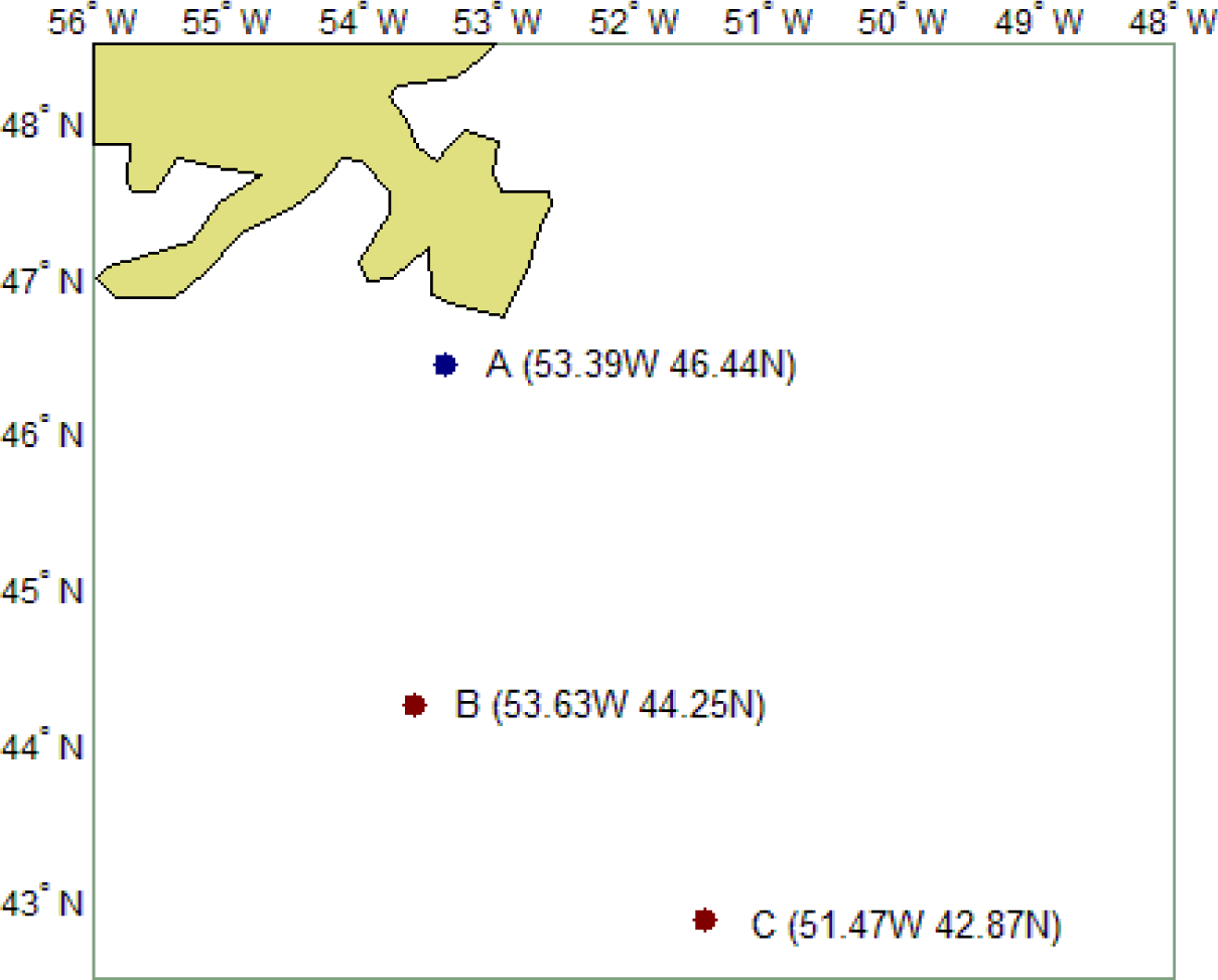
5.1. Buoy Data Set

To assess the performance of the proposed approach for reconstructing wind field, the retrieved wind speeds are compared with buoy-measured wind speeds. The buoy wind measurements are generally reported on the hour and represent 10-min averages. The reconstructed wind is averaged over 10 km in space and is a proxy point measurement in time.

Figure 1 shows the area coverage of reconstructed wind field and buoy locations used in the comparison. Since the anemometer on the buoys measures the wind speed at 5.2 m above the water surface, all the buoy data had to be converted to the equivalent neutral winds at 10 m for comparison. The Tropical Ocean Global Atmosphere Coupled Ocean Atmosphere Response Experiment (TOGA-COARE) bulk flux algorithm has been used for the stability correction [43].

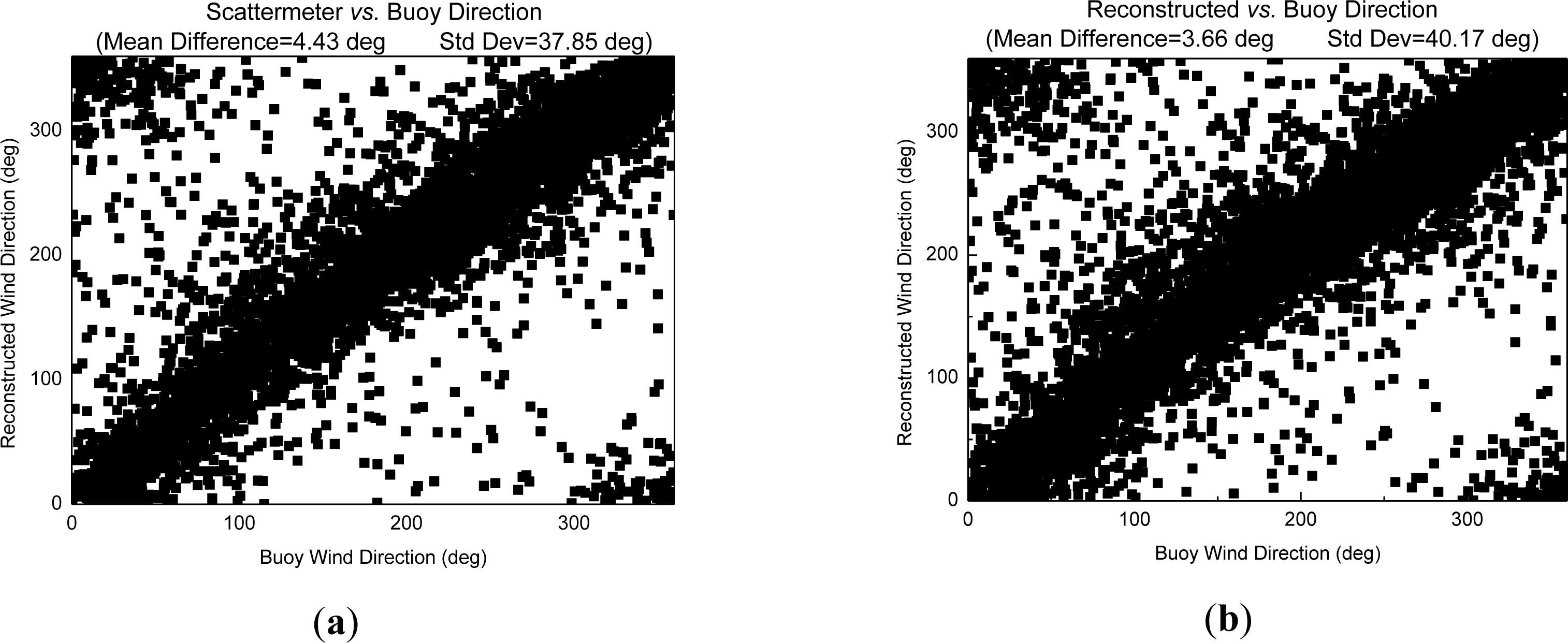
5.2. Wind Direction Comparisons

The SAR wind-speed retrieval depends on the near-real-time wind direction measurements interpolated from BP. Differences between the actual direction and the inferred wind direction from BP may contribute to those between SAR and buoy wind speeds. Sequentially, differences between reconstructed and buoy wind speeds would be affected.

Figure 2 shows scatter plots that respectively compare the BP and reconstructed wind directions with the buoy-estimated ones. The mean difference in wind direction between the reconstructed and buoy estimates is 3.7°, smaller than that between BP and the buoy by 0.8°. However, the standard deviation of the difference between the reconstructed and buoy estimates is 40.2°, 2.3° greater than that between BP and buoy estimates.

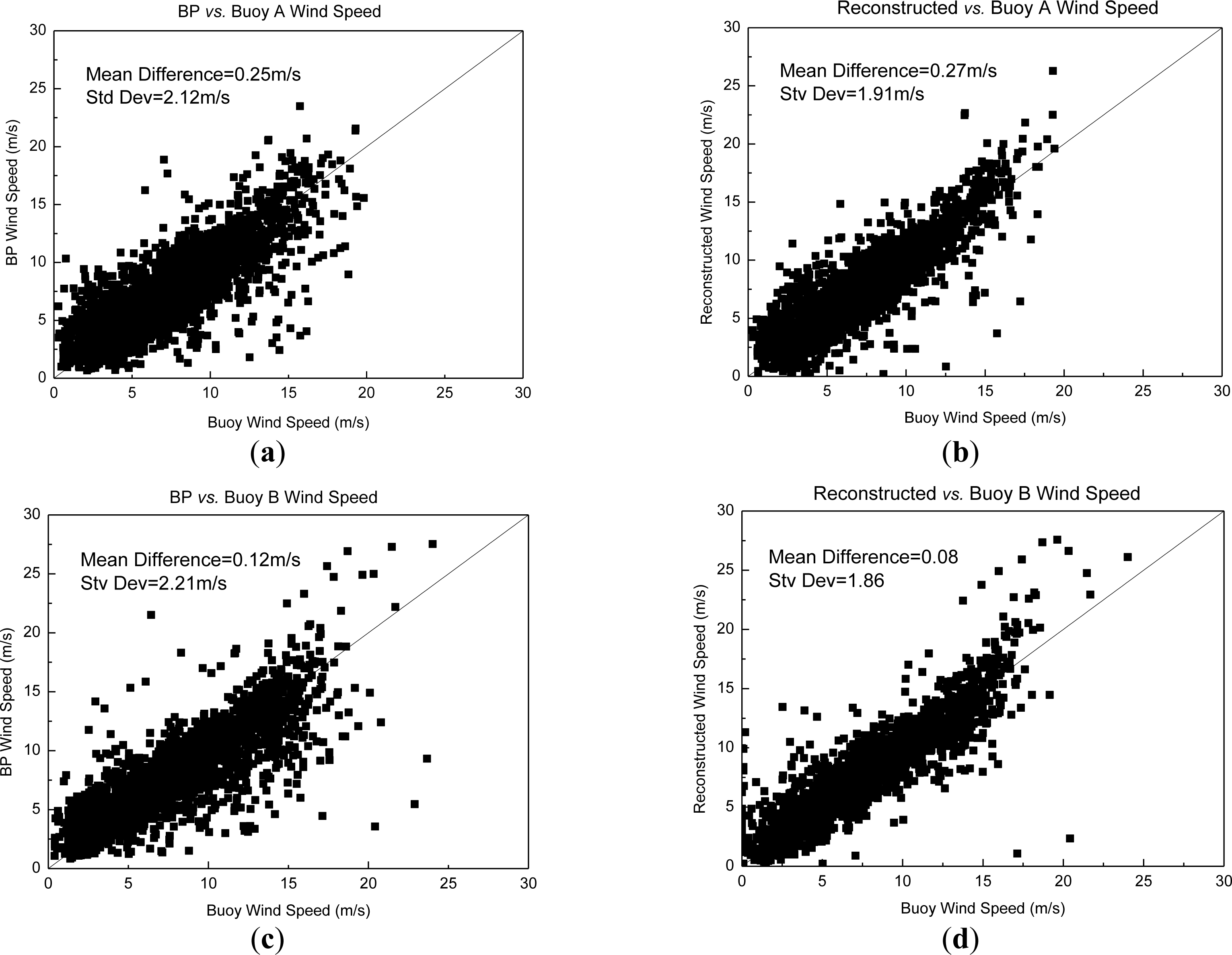
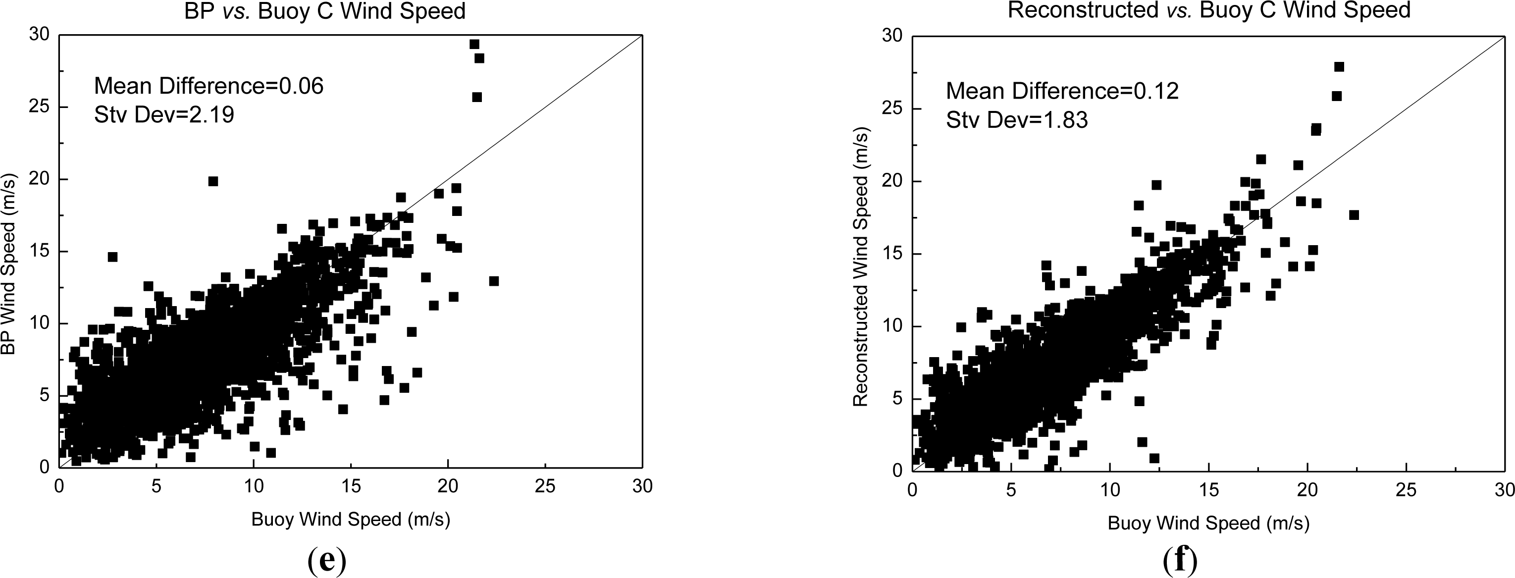
5.3. Differences between Buoy and Reconstructed Wind Speeds

The number of available observations for comparisons from the A, B and C buoy is 2688, 2568 and 2480 respectively. Figure 3 shows the reconstructed and BP wind speeds vs. the buoy-measured wind speed for each buoy. The mean difference and the standard deviation are also indicated in the figures. The mean difference between the BP wind speed and buoy measurements is smaller than 0.25 m/s, and the standard deviation is smaller than 2.21 m/s. The mean difference between the reconstructed wind speed and buoy measurements are approximately equal to that between the BP and buoy measurements. However, the standard deviation between the reconstructed wind speed and buoy measurements has been improved.

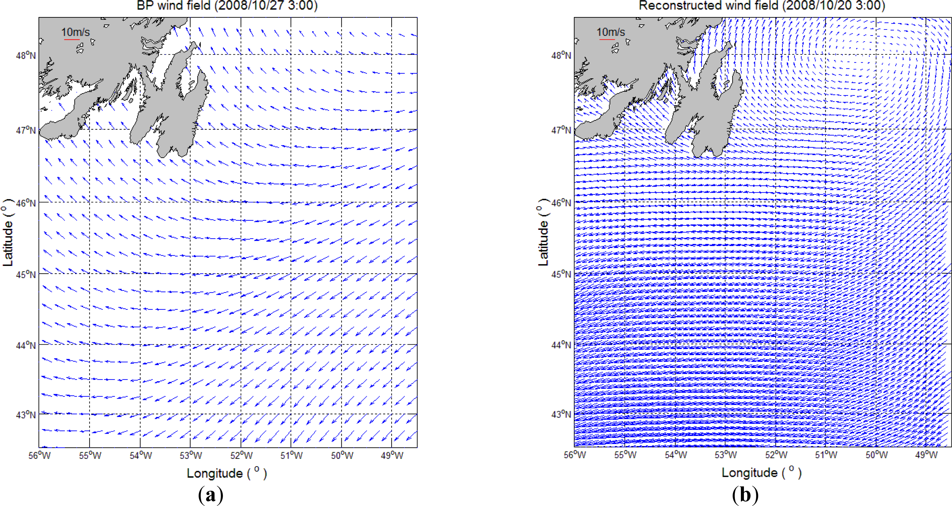
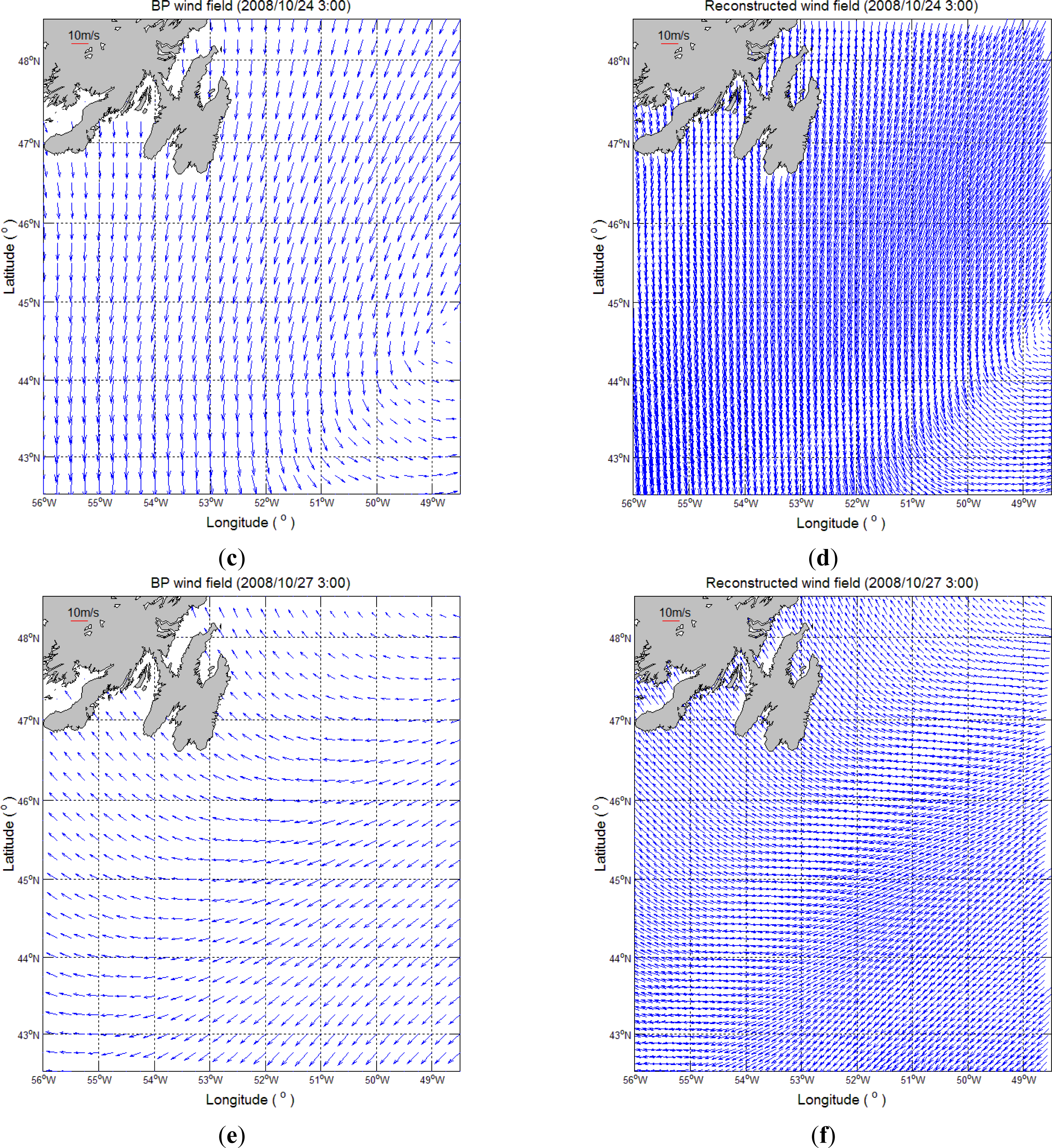
5.4. Comparison between the BP and Reconstructed Wind Fields

The reconstructed wind fields at 3:00 on 20, 24 and 27 October have been chosen for comparison with the BP wind fields, because near-real-time SAR wind fields were obtained on those dates. Figure 4 shows that there is overall consistency in wind regime between the BP wind fields and reconstructed wind fields. The wind vortex at the top right corner of Figure 4b, a sudden change in the direction of the wind at the bottom right corner of Figure 4d and the gradual change in the direction of the wind in Figure 4f have been described in more detail in the reconstructed data. Fine-scale wind features near the coast have also been shown in Figure 4d–f.

6. Conclusion

In this paper, the six-hourly lower spatial resolution wind fields from BP and irregular higher spatial resolution wind fields derived from SAR images have been blended to reconstruct wind fields. Both the resolution and regularities of wind fields have been taken into account in the study.

The comparison of reconstructed wind speeds and buoy measurements shows good agreement for both wind speed and direction. The mean difference in wind direction between reconstructed and buoy estimates is 3.7°, the standard deviation is 40.2°. The mean difference in wind direction between reconstructed and buoy estimates is 0.8° lower than the mean difference in wind direction between BP and buoy estimates. However, the standard deviation is 2.3° greater than the mean difference in wind direction between reconstructed and buoys estimates.

The accuracy of the wind speed has been improved a little, because the standard deviation between the reconstructed wind speed and buoy measurements is less than the one between the BP wind speed and buoys measurement. The comparison of the reconstructed wind fields with the BP wind fields shows a preferable identity and suggests that the results are reasonable and reliable. Higher spatial resolution regular wind fields have been obtained successfully.

The results suggest that the joint GMF-PR approach (CMOD5.N-SAD) constitutes a promising hybrid model for wind speed retrievals from HH-polarized RADARSAT-2 SAR images, and the reconstruction process based on the heapsort bucket method with topdown search and the modified Gauss–Markov theory is practicable. There are a number of factors for the residual differences between the reconstructed and buoy wind speed measurements. For example, the residual differences may in part come from BP. The CMOD5.N and polarization ratio functions used here may be further refined. More SAR images should be acquired in this reconstruction process.

References and Notes

1. Christiansen, M.B.; Koch, W.; Horstmann, J.; Bay Hasager, C.; Nielsen, M. Wind resource assessment from C-band SAR. Remote Sens Environ 2006, 105, 68–81. [Google Scholar]
2. Christiansen, M.B. Wind Energy Applications of Synthetic Aperture Radar; Risø National Laboratory: Roskilde, Denmark, 2006. [Google Scholar]
3. Elfouhaily, T. Physical Modeling of Electromagnetic Backscatter from the Ocean Surface; Application to Retrieval of Wind Fields and Wind Stress by Remote Sensing of the Marine Atmospheric Boundary Layer. Ph.D. Thesis, Dépt d’Océanogr Spatiale, l’Inst Français Rec l’Exploitation Mer (IFREMER), Plouzane, France,. 1997. [Google Scholar]
4. McCollum, J.R.; Ferraro, R.R. Next generation of NOAA/NESDIS TMI, SSM/I, and AMSR-E microwave land rainfall algorithms. J. Geophys. Res.: Atmos 2003. [Google Scholar] [CrossRef]
5. Wentz, F.J.; Spencer, R.W. SSM/I rain retrievals within a unified all-weather ocean algorithm. J Atmos Sci 1998, 55, 1613–1627. [Google Scholar]
6. Surussavadee, C.; Staelin, D.H.; Chadarong, V.; McLaughlin, D.; Entekhabi, D. Comparison of NOWRAD, AMSU, AMSR-E, TMI, and SSM/I Surface Precipitation Rate Retrievals over the United States Great Plains. In Proceeding of the 2007 IEEE International Geoscience and Remote Sensing Symposium, Barcelona, Spain, 23–28 July 2007; pp. 3923–3926.
7. Zhang, H.-M.; Bates, J.J.; Reynolds, R.W. Assessment of composite global sampling: Sea surface wind speed. Geophys. Res. Lett 2006. [Google Scholar] [CrossRef]
8. Zhang, H.; Reynolds, R.; Bates, J. Blended and Gridded High Resolution Global Sea Surface Wind Speed and Climatology from Multiple Satellites: 1987–Present. In Proceeding of American Meteorological Society 006 Annual Meeting, Atlanta, GA, America, 29 January–2 February 2006; p. 2.23.
9. Stoffelen, A. Toward the true near-surface wind speed: Error modeling and calibration using triple collocation. J. Geophys. Res.: Ocean 1998, 103, 7755–7766. [Google Scholar]
10. Spencer, M.W.; Chialin, W.; Long, D.G. Improved resolution backscatter measurements with the SeaWinds pencil-beam scatterometer. IEEE Trans. Geosci. Remote Sens 2000, 38, 89–104. [Google Scholar]
11. Monaldo, F.M.; Thompson, D.R.; Pichel, W.G.; Clemente-Colon, P. A systematic comparison of QuikSCAT and SAR ocean surface wind speeds. IEEE Trans. Geosci. Remote Sens 2004, 42, 283–291. [Google Scholar]
12. Pospelov, M.N. Wind direction signal in polarized microwave emission of sea surface under various incidence angles. Gayana (Concepción) 2004, 68, 493–498. [Google Scholar]
13. Wentz, F.J. A well calibrated ocean algorithm for special sensor microwave/image. J. Geophys. Res 1997, 102, 8703–8718. [Google Scholar]
14. Wentz, F.J. SSM/I Version-7 Calibration Report; RSS Technical Report 011012; Remote Sensing Systems: Santa Rosa, CA, USA, 2013. [Google Scholar]
15. Gentemann, C.L.; Meissner, T.; Wentz, F.J. Accuracy of satellite sea surface temperatures at 7 and 11 GHz. IEEE Trans. Geosci. Remote Sens 2010, 48, 1009–1018. [Google Scholar]
16. Wentz, F.J.; Ashcroft, P.; Gentemann, C. Post-launch calibration of the TRMM microwave imager. IEEE Trans. Geosci. Remote Sens 2001, 39, 415–422. [Google Scholar]
17. Hilburn, K.; Wentz, F. Intercalibrated passive microwave rain products from the Unified Microwave Ocean Retrieval Algorithm (UMORA). J. Appl. Meteorol. Clim 2008, 47, 778–794. [Google Scholar]
18. Pospelov, M.N. Surface wind speed retrieval using passive microwave polarimetry: The dependence on atmospheric stability. IEEE Trans. Geosci. Remote Sens 1996, 34, 1166–1171. [Google Scholar]
19. Flett, D.G.; Wilson, K.J.; Vachon, P.W.; Hopper, J.F. Wind information for marine weather forecasting from RADARSAT-1 synthetic aperture radar data: Initial results from the “Marine winds from SAR” demonstration project. Can. J. Remote Sens 2002, 28, 490–497. [Google Scholar]
20. Horstmann, J.; Koch, W.; Lehner, S.; Tonboe, R. Ocean winds from RADARSAT-1 ScanSAR. Can. J. Remote Sens 2002, 28, 524–533. [Google Scholar]
21. Vachon, P.W.; Wolfe, J.; Hawkins, R.K. Comparison of C-band wind retrieval model functions with airborne multipolarization SAR data. Can. J. Remote Sens 2004, 30, 462–469. [Google Scholar]
22. Hersbach, H.; Stoffelen, A.; de Haan, S. An improved C-band scatterometer ocean geophysical model function: CMOD5. J. Geophys. Res.: Ocean 2007. [Google Scholar] [CrossRef]
23. Horstmann, J.; Schiller, H.; Schulz-Stellenfleth, J.; Lehner, S. Global wind speed retrieval from SAR. IEEE Trans. Geosci. Remote Sens 2003, 41, 2277–2286. [Google Scholar]
24. Monaldo, F.; Kerbaol, V.; Clemente-Colón, P.; Furevik, B.; Horstmann, J.; Johannessen, J.; Li, X.; Pichel, W.; Sikora, T.; Thomson, D. The SAR Measurement of Ocean Surface Winds: An Overview. In Proceedings of the Second Workshop Coastal and Marine Applications of SAR, Svalbard, Norway, 8–12 September 2003; pp. 2–12.
25. Koch, W. Directional analysis of SAR images aiming at wind direction. IEEE Trans. Geosci. Remote Sens 2004, 42, 702–710. [Google Scholar]
26. Fetterer, F.; Gineris, D.; Wackerman, C.C. Validating a scatterometer wind algorithm for ERS-1 SAR. IEEE Trans. Geosci. Remote Sens 1998, 36, 479–492. [Google Scholar]
27. Gerling, T.W. Structure of the surface wind field from the Seasat SAR. J. Geophys. Res.: Ocean 1986, 91, 2308–2320. [Google Scholar]
28. Lehner, S.; Horstmann, J.; Koch, W.; Rosenthal, W. Mesoscale wind measurements using recalibrated ERS SAR images. J. Geophys. Res.: Ocean 1998, 103, 7847–7856. [Google Scholar]
29. Du, Y.; Vachon, P.W.; Wolfe, J. Wind direction estimation from SAR images of the ocean using wavelet analysis. Can. J. Remote Sens 2002, 28, 498–509. [Google Scholar]
30. Stoffelen, A.; Anderson, D. Scatterometer data interpretation: Estimation and validation of the transfer function CMOD4. J. Geophys. Res.: Ocean 1997, 102, 5767–5780. [Google Scholar]
31. Quilfen, Y.; Chapron, B.; Elfouhaily, T.; Katsaros, K.; Tournadre, J. Observation of tropical cyclones by high-resolution scatterometry. J. Geophys. Res.: Ocean 1998, 103, 7767–7786. [Google Scholar]
32. Herbach, H. CMOD5: A C-band Geophysical Model Function for Equivalent Neural Wind; Technical Memorandum No. 554; European Centre for Medium-Range Weather Forecasts: Reading, UK, 2008. [Google Scholar]
33. Herbach, H. Comparison of C-band scatterometer CMOD5.N equivalent neural winds with ECMWF. J. Atmos. Oceanic. Technol 2010. [Google Scholar] [CrossRef]
34. Horstmann, J.; Koch, W. Measurement of ocean surface winds using synthetic aperture radars. IEEE J. Oceanic Eng 2005, 30, 508–515. [Google Scholar]
35. Monaldo, F.M.; Thompson, D.R.; Beal, R.C.; Pichel, W.G.; Clemente-Colon, P. Comparison of SAR-derived wind speed with model predictions and ocean buoy measurements. IEEE Trans. Geosci. Remote Sens 2001, 39, 2587–2600. [Google Scholar]
36. Horstmann, J.; Koch, W.; Lehner, S.; Tonboe, R. Wind retrieval over the ocean using synthetic aperture radar with C-band HH polarization. IEEE Trans. Geosci. Remote Sens 2000, 38, 2122–2131. [Google Scholar]
37. Vachon, P.W.; Dobson, F.W. Wind retrieval from RADARSAT SAR images: Selection of a suitable C-band HH polarization wind retrieval model. Can. J. Remote Sens 2000, 26, 306–313. [Google Scholar]
38. Johnsen, H.; Engen, G.; Guitton, G. Sea-surface polarization ratio from Envisat ASAR AP data. IEEE Trans. Geosci. Remote Sens 2008, 46, 3637–3646. [Google Scholar]
39. Mouche, A.A.; Hauser, D.; Daloze, J.F.; Guerin, C. Dual-polarization measurements at C-band over the ocean: Results from airborne radar observations and comparison with ENVISAT ASAR data. IEEE Trans. Geosci. Remote Sens 2005, 43, 753–769. [Google Scholar]
40. Thompson, D.R.; Elfouhaily, T.M.; Chapron, B. Polarization Ratio for Microwave Backscattering from the Ocean Surface at Low to Moderate Incidence Angles. In Proceedings of the 1998 IEEE International Geoscience and Remote Sensing Symposium, Seattle, WA, USA, 6–10 July 1998.
41. Unal, C.M.H.; Snoeij, P.; Swart, P.J.F. The polarization-dependent relation between radar backscatter from the ocean surface and surface wind vector at frequencies between 1 and 18 GHz. IEEE Trans. Geosci. Remote Sens 1991, 29, 621–626. [Google Scholar]
42. Zhang, B.; Perrie, W.; He, Y. Wind speed retrieval from RADARSAT-2 quad-polarization images using a new polarization ratio model. J. Geophys. Res.: Ocean 2011. [Google Scholar] [CrossRef]
43. Fairall, C.W.; Bradley, E.F.; Rogers, D.P.; Edson, J.B.; Young, G.S. Bulk parameterization of air-sea fluxes for tropical ocean-global atmosphere coupled-ocean atmosphere response experiment. J. Geophys. Res.: Ocean 1996, 101, 3747–3764. [Google Scholar]
Figure 1. Geographic location of the three buoys for comparison with reconstructed wind vectors.
Remotesensing 06 02898f1
Figure 2. (a) Blended products (BP) vs. buoy wind directions (Buoys A + B + C). (b) Reconstructed vs. buoy wind directions (Buoys A + B + C).
Remotesensing 06 02898f2
Figure 3. (a) BP vs. Buoy A-estimated wind speeds. (b) Reconstructed vs. Buoy A-estimated wind speeds. (c) BP vs. Buoy B-estimated wind speeds. (d) Reconstructed vs. Buoy B-estimated wind speeds. (e) BP vs. Buoy C-estimated wind speeds. (f) Reconstructed vs. Buoy C-estimated wind speeds.
Remotesensing 06 02898f3aRemotesensing 06 02898f3b
Figure 4. (a) BP wind field at 03:00, 20 October 2008. (b) Reconstructed wind field at 03:00, 20 October 2008. (c) BP wind field at 03:00, 24 October 2008. (d) Reconstructed wind field at 03:00, 24 October 2008. (e) BP wind field at 03:00, 27 October 2008. (f) Reconstructed wind field at 03:00, 27 October 2008.
Remotesensing 06 02898f4aRemotesensing 06 02898f4b