Performance Evaluation of Machine Learning Algorithms for Urban Pattern Recognition from Multi-spectral Satellite Images

Abstract

In this study, a classification and performance evaluation framework for the recognition of urban patterns in medium (Landsat ETM, TM and MSS) and very high resolution (WorldView-2, Quickbird, Ikonos) multi-spectral satellite images is presented. The study aims at exploring the potential of machine learning algorithms in the context of an object-based image analysis and to thoroughly test the algorithm’s performance under varying conditions to optimize their usage for urban pattern recognition tasks. Four classification algorithms, Normal Bayes, K Nearest Neighbors, Random Trees and Support Vector Machines, which represent different concepts in machine learning (probabilistic, nearest neighbor, tree-based, function-based), have been selected and implemented on a free and open-source basis. Particular focus is given to assess the generalization ability of machine learning algorithms and the transferability of trained learning machines between different image types and image scenes. Moreover, the influence of the number and choice of training data, the influence of the size and composition of the feature vector and the effect of image segmentation on the classification accuracy is evaluated.

1. Introduction

Extraction of information on the built environment from remote sensing imagery is a complex task, mainly due to the manifold combinations of surface materials and the diversity of size, shape and placement of the objects composing a typical image scene. It is increasingly being recognized that image domains beyond spectral information, such as geometrical, temporal or textural domains must be utilized in order to tackle the complexity of the information extraction. In this regard, algorithms that make use of the extended information content of image segments (also referred to as super-pixels or objects) have been adapted by the remote sensing community in recent years [1]. Such an object-based image analysis emerged primarily in the context of Very High Resolution (VHR) image analysis (Ground Sampling Distance (GSD) < 1–4 m), where it showed advantages over pixel-based approaches [2] for extracting detailed thematic information such as single buildings or streets [3,4]. An object-based image analysis can also be beneficial, when analyzing the built environment from Medium Resolution (MR) satellite images (GSD 15–60 m) [5,6], where different urban patterns are mainly defined by the placement of buildings, streets and open-spaces and therefore cannot sufficiently be described by just the spectral values of a single pixel.

When segments are used as the basic spatial entity for analysis, a large number of image features can be generated to describe the objects of interest in an image. This includes spectral features such as mean and standard deviation values per image band, minimum and maximum pixel values, mean band ratios or mean and standard deviation of band indices such as the Normalized Difference Vegetation Index (NDVI) [7]. Textural features, which take into account neighborhood relations between pixels, can be effectively computed over the segments. Commonly used textural descriptors in remote sensing analysis include second-order texture features derived from the Gray-Level Co-occurrence Matrix (GLCM), such as angular second moment, entropy, contrast or correlation. A mathematical notation of the GLCM and the related second-order textural features is given in Haralick et al. [8]. A class of features unique to object-based approaches that has frequently claimed to provide major improvements in object recognition is geometrical features [1,9]. Geometrical features or shape descriptors can be generally divided into contour-based and region-based. Contour-based features are extracted from the contour of an object and include, amongst others, convexity, perimeter, compactness or major axis orientation. Region-based features are extracted from the shape region and include area, eccentricity or moment features like the Hu moments [10]. Reviews of shape representation and description techniques with mathematical explanations of the different mentioned descriptors can be found in [11,12].

To reduce the dimensionality of the feature space and preselect the most significant features for a specific classification task, dataset and classifier, several feature selection methods have been proposed in the literature [13,14]. The most commonly found method in remote sensing applications is a manual feature selection with conventional data exploration tools such as histograms or scatter-plots. This method requires a sound understanding of the classification task and the characteristics of the features under observation. However, increasing the number of features of manual methods becomes impracticable and more quantitative feature selection techniques are needed [15]. The ReliefF feature ranking algorithm for example has been widely used in other research fields such as medical imaging, and has been successfully applied to noisy and correlated datasets [14]. Despite its great potential, it has only rarely been used in remote sensing applications so far [16].

To partition a multi-dimensional feature space into homogeneous areas and therefore to label segments with respect to desired classes, several image classification algorithms are available, commonly categorized into parametric and non-parametric classifiers. Parametric classifiers assume a normally distributed dataset and statistical parameters are directly inferred from training data [4]. A parametric classifier, which has been widely used in remote sensing application, is the Normal Bayes classifier. Non-parametric classifiers do not assume a specific data distribution to separate a multi-dimensional feature space into classes. Most commonly used non-parametric classifiers include Decision Trees, Support Vector Machines and Expert Systems. It can be inferred from the literature that machine learning algorithms (both parametric and non-parametric) have mainly been used as per-pixel classifiers in remote sensing image analysis [4]. For the classification of image segments, many studies so far have used fuzzy set theory-based expert systems [17,18]. Expert systems are considered to have a great potential for image classification when also considering ancillary data [4]. However, a critical part of such systems is the development of rule sets to describe the classes of interest. Often threshold values need to be manually adjusted and classification rules are strongly bound to a particular image scene and image type. Only a few studies have designed generalized rule sets that aim at being transferable [3]. The application of machine learning algorithms in the context of an object-based image analysis has only rarely been tested [19] and further research in this direction is advocated. In particular, the potential of applying pre-trained learning machines to different image types and image scenes should be further assessed. While most pattern recognition methods in remote sensing are trained and tested on the same image distribution, real-world applications often involve changing visual domains (e.g., multi-temporal change detection, regional landuse/landcover mapping). In general, satellite image distributions could differ in combinations of partially uncontrollable or unknown factors, including atmospheric effects, sensor gain or seasonal variations in the image scene. Recent studies have proposed the use of domain adaptation [20], retraining [21] or multi-task learning [22] techniques to improve the transferability of pixel-based classifications in the spectral domain. The question of transferability of classifiers on an extended and partly domain-invariant feature space derived from an object-based image analysis remains still largely unanswered in remote sensing applications.

The objectives of this study are to develop a method and the related software tools based on Free and Open-Source Solutions (FOSS) for the recognition of urban patterns in multi-spectral satellite images. Four machine learning classification algorithms (Normal Bayes, K Nearest Neighbors, Random Trees and Support Vector Machines) are implemented and thoroughly tested for their performance under varying conditions to optimize their usage and assess their applicability in the context of an object-based image analysis. In particular, the following research questions are addressed:

(1)

What are the most important image features for class separability?

(2)

How sensitive are learning machines to the size of the feature vector?

(3)

How does the number of training instances influence the performance of the learning machines?

(4)

How well can a trained learning machine be transferred between different image types and image scenes?

(5)

How does image segmentation influence the classification results?

The goal is to develop classifiers for the recognition of built-up areas from different MR and VHR image types that are able to maximize true positive and true negative detection rates, while minimizing the number of input features and training instances to reduce computation time and training efforts. It is furthermore desirable that a trained learning machine can be transferred between different image types and image scenes to reduce the effort of manually selecting training instances and therefore to maximize the level of automation of the classification procedure.

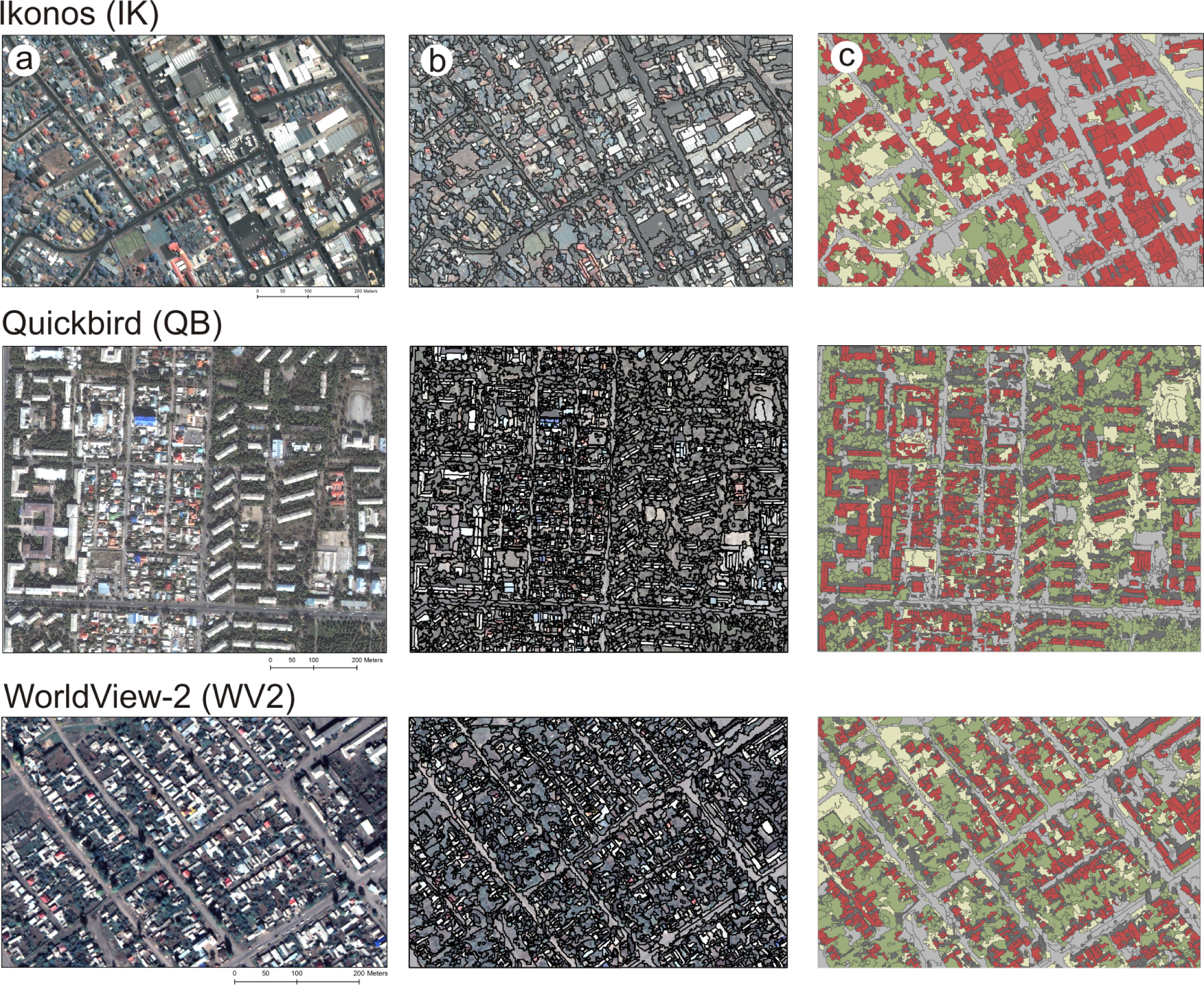
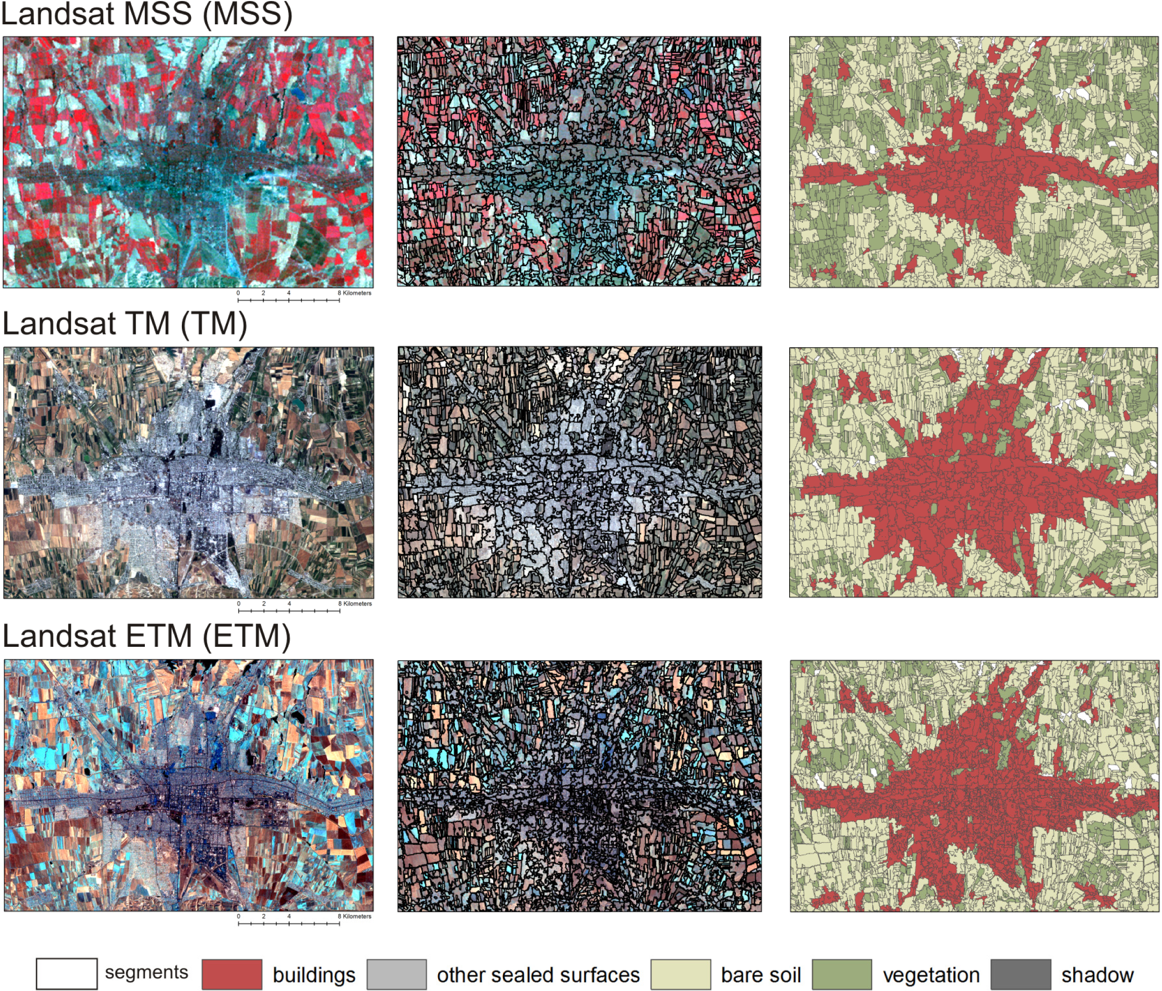
2. Data Specifications and Preprocessing

To train and test classification algorithms under varying conditions, six subsets of different multi-spectral satellite image types are used in the following (Figure 1a). Details about the specific images, including spectral, radiometric and geometric properties, acquisition date, subset area and applied image preprocessing steps are listed in

Table 1. Satellite images, their specifications and applied preprocessing steps.

Image	Type	Spectral Res. (μm)	Radiom. Res. (bit)	Geom. Res. (m)	Size (px)	Date Coverage	Preprocessing
IK	Ikonos	0.45–0.9 (4 bands)	11	1 (pan) 4 (mul)	800 × 500	22.02.03 Hobart	pan-sharpened
QB	Quickbird	0.45–0.90 (4 bands)	11	0.6 (pan) 2.4 (mul)	1500 × 1200	29.09.09 Bishkek	pan-sharpened
WV2	WorldView-2	0.45–0.89 (4 bands)	11	0.5 (pan) 2.4 (mul)	1200 × 800	12.10.11 Karakol	pan-sharpened
MSS	Landsat MSS	0.52–1.10 (4 bands)	8	60 (mul)	1000 × 700	22.08.77 Bishkek	-
TM	Landsat TM	0.45–12.5 (7 bands)	8	30 (mul) 120 (TIR)	1000 × 700	08.07.09 Bishkek	resampled to 30m (TIR)
ETM	Landsat ETM	0.45–12.5 (7 bands)	8	15 (pan) 30 (mul) 60 (TIR)	2000 × 1200	14.08.01 Bishkek	pan-sharpened, resampled to 15 m (TIR)

. All images have been layer-stacked, georectified and when covering the same spatial subset have been co-registered to each other. In case of resampling operations, a nearest neighbor algorithm has been applied since it is the interpolator that alters the spectral values the least [23]. For image fusion of multi-spectral and panchromatic bands (pan-sharpening), the Brovey transform, which is implemented in GRASS [24], has been used. The Brovey transform [25] is a color transform algorithm that normalizes the lower resolution multi-spectral image bands and multiplies the result with a higher resolution (panchromatic) band.

For each image subset, a reference dataset has been compiled. The images have been segmented using an efficient graph-based segmentation algorithm [26] (see also Section 3) (Figure 1b) and the resulting segments have been manually labeled based on visual interpretation of the satellite image to create the reference datasets (Figure 1c). For the VHR satellite images (Quickbird (QB), WorldView-2 (WV2) and Ikonos (IK) [27]), landcover classes were organized in two groups: (1) “built-up areas” (“buildings”) and (2) “not built-up areas” (“vegetation”, “bare soil”, “shadow”, “other sealed surfaces”). For the MR images (Landsat Enhanced Thematic Mapper (ETM), Landsat Thematic Mapper (TM) and Landsat Multi-Spectral Scanner (MSS)), three landcover classes (“built-up areas”, “vegetation” and “other not built-up areas”) were organized in the two groups and reference datasets were created in the same way through manual labeling of image segments.

3. Image Segmentation and the Scale of Analysis

Image segmentation clusters the original image pixels into segments, based on one or more criteria of similarity in one or more dimensions of a feature space, and is a preliminary and crucial step in object-based image analysis [1]. An efficient graph-based image segmentation algorithm, which has been originally developed by Felzenszwalb and Huttenlocher [26], is used within this study. The algorithm measures the evidence for a boundary between two segments by comparing the feature vectors across the boundary with those between neighboring pixels within each segment. The brightness values of the image pixels in all spectral bands of the satellite image are used to define the input feature space for segmentation, and the L2 Euclidean distance is used to measure the dissimilarity. A threshold function with runtime parameters k (scale parameter) and m (minimum allowable segment size) allow to effectively set a spatial scale of analysis, since larger values for k and m favor larger segments.

Ideal segments are considered as singular entities outlining objects of homogeneous appearance without over- or under-segmenting them. To define the scale of analysis, segmentation parameters must be adjusted and quantitative evaluation of the segmentation quality becomes important. In this study, segmentation parameters for the VHR images have been adjusted based on a comparison of the segmentation results with reference objects by using supervised segmentation quality measures [28]. In a set of segmentations, the parameter values that produced the best area-fit to the reference objects with the least number of segments where selected.

Compared to VHR images where analysis scales can be defined by comparing the segmentations with reference objects, the delineation of reference objects in MR images is problematic due to their large GSD. Given a GSD in a range of 15–60 m for Landsat imagery, individual buildings cannot be detected. However, larger morphological units that are composed of a mixture of buildings, streets and open-space can be distinguished from this image type. Such units cannot be delineated solely based on geometrical properties, but are mainly defined by spectral and textural image properties. This makes the manual delineation of reference objects difficult and potentially strongly biased from an operator’s point of view. It emphasizes that segmentation quality needs to be assessed in an unsupervised way using image statistics. A generally accepted segmentation quality measure is based on the comparison of intra-segment homogeneity and inter-segment heterogeneity [29]. In a set of segmentations, the segmentation that minimizes intra-segment variability and maximizes inter-segment separability is defined as being optimal in terms of providing the most appropriate analysis scale for a given image scene. A global Moran’s I has been utilized to quantify inter-segment heterogeneity. The standard deviation of the brightness values of the input image bands, weighted by each segment’s size and summed over all the segments in the image scene, has been used for assessing intra-segment homogeneity [30]. Parameter values resulting in the segmentation with largest inter-segment heterogeneity and intra-segment homogeneity have been selected.

4. Classification Algorithms

The classification algorithms, which have been implemented in this study, represent the state-of-the-art in machine learning and are based on different concepts (probabilistic, nearest neighbor, tree-based, function-based). The implemented classification algorithms are based on OpenCV solutions [31] and are briefly described in the following. Common to all the classifiers is that they make use of training samples. The basic structure of a training sample in remote sensing consists of a point-location with an associated class label, which has been identified and defined by an expert, usually based on either ground-truth knowledge or visual image interpretation. Once a training dataset is defined in its basic structure, it can be used to train a classifier on any kind of input image type and feature space.

4.1. Normal Bayes (NB)

Normal Bayes (NB) is a simple probabilistic classification model that assumes the normal distribution of the feature space for each class. This means that the whole data distribution function is assumed to be a Gaussian mixture with one component per class [31]. Based on selected training instances, the NB algorithm estimates mean vectors and covariance matrices for each class and utilizes them for predictions. A detailed mathematical description of the classification model can be found, for example, in Fukunaga [32].

4.2. K Nearest Neighbors (KNN)

The K Nearest Neighbors (KNN) classification model classifies for each unlabeled instance its k nearest neighbors in the multi-dimensional feature space spanned by a set of training instances and assigns a class value according to the majority of a particular class within this neighborhood. The k nearest neighbors are identified by a distance measure that compares the feature vectors of the unlabeled instance and the set of training instances provided to the classifier. Once a list of nearest neighbors is obtained, the prediction is based on voting (majority or distance-weighted) [33].

4.3. Random Trees (RT)

Random Trees (RT) are also referred to as random forests and have been introduced by Leo Breiman and Adele Cutler [34,35] as an ensemble of decision tree (DT) classifiers. DT use a chain of simple decisions based on the results of sequential tests for class label assignment. The branches of the DT are composed of sets of decision sequences where tests are applied at the nodes of the tree and the leaves represent the class labels. To construct a DT, a training dataset is recursively split into increasingly homogeneous subsets based on tests that are applied to one or more values of the input feature vector. Prediction or label assignment is performed at the end nodes of the tree (leaves) by using an allocation strategy [36]. In RT, the input feature vector is classified with every tree in the forest where the final prediction is based on a majority voting. The trees are trained with the same parameters, but with different sets of training instances. The training sets are selected by using a bootstrap procedure on the original training dataset where for each training set the same number of vectors as in the original set is randomly selected with replacement. A random subset of the variables is used at each node of the trained trees to find the best split. The size of subsets generated at each node is fixed for all the nodes and trees by a training parameter. None of the trees that are built are pruned [31]. The classification error for each tree is estimated from out-of-bag data, which is compiled by vectors that were left out during the training phase of the single tree classifiers by sampling with replacement.

4.4. Support Vector Machine (SVM)

A Support Vector Machine (SVM) is a classifier derived from statistical learning theory and was originally developed by Vladimir Vapnik [37,38]. SVM separates any two classes of interest by identifying an optimal linear separating hyperplane. A kernel function is used to project non-linearly separable classes from the original feature space to a higher dimensional space, where the non-linearly separable classes can be separated by a linear hyperplane. To choose the optimal separating hyperplane between two classes, SVM utilizes the maximum margin concept, which maximizes the margin between the separating hyperplane and the closest feature vectors. These feature vectors are called “support vectors”, meaning that the position of other feature vectors does not affect the hyperplane. Selecting this particular hyperplane maximizes the ability of the SVM to predict the correct class of previously unseen samples. Furthermore, a soft-margin parameter is introduced in SVM to deal with outliers in the data, which allows some data points to violate the separation through the hyperplane without affecting the final result. Therefore, the soft-margin parameter determines a trade-off between the size of the margin and the hyperplane violations. As the SVM classifier is dependent on a distance measure, it is important to account for the normalization of the feature variables by their average variance or covariance. To apply SVM to multi-class problems, a simple and commonly used generalization method is to train multiple, one-versus-all classifiers. Optimal SVM parameters are selected according to a standard ten-fold cross-validation method during the training phase of the classifier. Using a k-fold cross-validation moreover decreases the risk of over-fitting [39].

5. Performance Evaluation of Classification Algorithms

To assess the performance of classifiers and to select the most appropriate classifier for a given task and image type (here, the recognition of built-up areas from MR and VHR satellite images), several experiments were carried out on the reference datasets. For performance evaluation, commonly used accuracy measures (sensitivity, specificity and overall accuracy) were estimated using a ten-fold cross-validation. Overall accuracy is defined as the total number of correctly classified segments divided by the total number of test segments. Sensitivity, also referred to as the true positive rate or producer’s accuracy, means the proportion of actual positives, which are classified as positives. Specificity, also referred to as true negative rate or user’s accuracy, is the proportion of actual negatives, which are classified as negatives. A random stratification procedure was used on the reference datasets to produce ten unique datasets for training (80%) and testing (20%) for each image type and image scene. Accuracy measures were averaged for each classification and the same training and testing datasets were used to train and test the four classifiers under different conditions, thus making it possible to assess the relative performance and consistency of the algorithms for a given task. The conditions for training and testing the classifiers were varied depending on the evaluation criteria which include the impact of feature selection, the impact of number and choice of training instances, the transferability of trained learning machines between different image types and image scenes and the effect of image segmentation on the classification results.

The following experiments have been carried out for each image subset on the basis of the same segmentation result that has been used to create the according reference dataset. In this way, only the labeling performance of the classifiers is evaluated and not the real map accuracy, which can be considered a product of both the segmentation and classification results. The real map accuracy would include also geometrical accuracy of extracted objects originating from the segmentation stage. The influence of the segmentation on the classification performance is evaluated separately in Subsection 5.5. Since reference labels are based on visual image interpretation, derived accuracy measures give indication on the labeling performance of learning machines relative to the performance of an experienced human operator. In the context of this work, this is desirable as it allows to isolate thematic labeling performance from geometric segmentation performance and information content of the image from real-world objects.

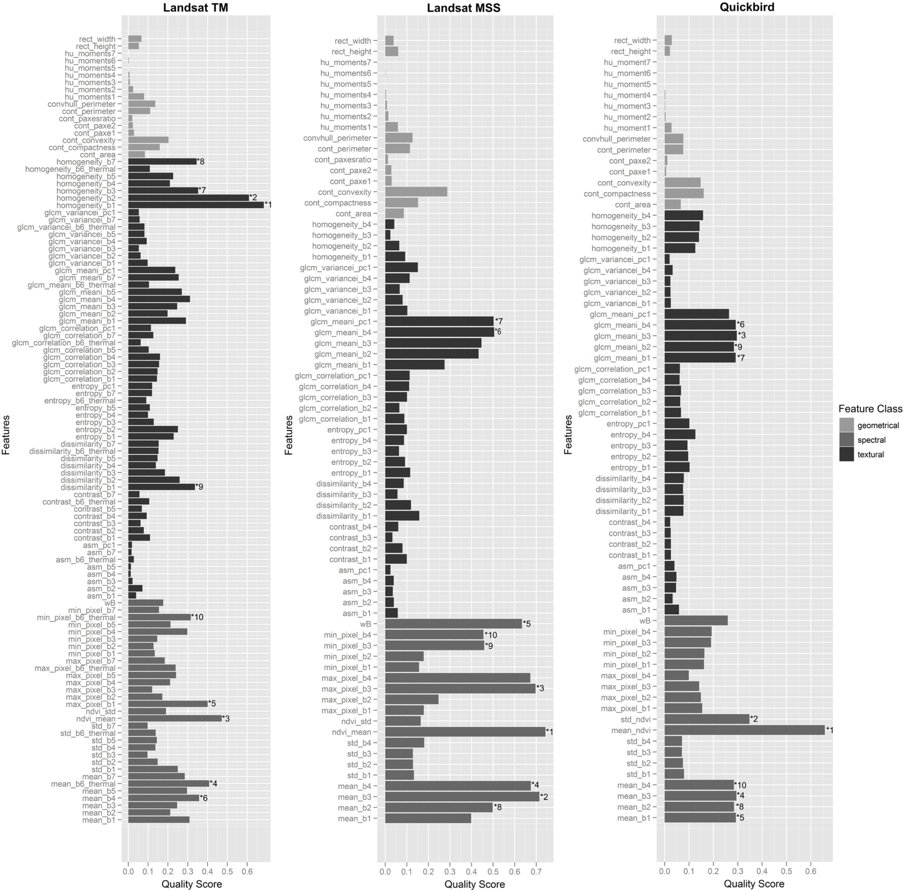
5.1. What are the Most Important Image Features for Class Separability?

A large set of image features used to describe segments in the spectral, textural and geometrical domain has been implemented based on custom C/C++ solutions and OpenCV functions. A large number of features may be beneficial in describing the segments with respect to classes of interest. However, redundant or irrelevant features that provide little information for a specific classification task can have a negative effect on machine learning models and can lead to a decrease in classification performance [15]. Moreover, the size of the feature vector clearly influences the computation time for feature calculation and for training the classifier. During the training stage of a classifier, machine learning algorithms themselves already select features and ignore irrelevant or redundant ones. However, it has been shown that in practice, the classification performance can be improved by a preselection of features before training [15]. In the following, the instance-based feature ranking algorithm ReliefF [40] was utilized to rank sets of features derived for different image types based on how well they distinguish between instances that are near to each other. An instance in this context is composed of a feature vector and an associated class label. ReliefF iteratively selects randomly m times an instance R from the data and finds its k nearest neighbors H from the same class (nearest hits) and k nearest neighbors M from the other classes (nearest misses). The feature values of R are compared to H and M and a quality score is adjusted with every iteration for the features depending on how well they separate the classes. If the feature values of R and H are different and therefore the feature separates instances from the same class, the quality score for this feature is decreased since this is not desirable. On the contrary, if the feature values of R and M are different and therefore the feature separates instances from different classes, which is desirable, the quality score is increased for this feature [14].

The ReliefF algorithm which is implemented in the open-source data mining software WEKA 3 [41] was used on the QB, TM and MSS reference datasets. The number of nearest neighbors has been set to k = 10 as suggested in [42] and the number of iterations has been set to m = all instances. Figure 2 gives an overview of the derived features for the different reference datasets grouped into spectral, textural and geometrical features and ranked by their importance in distinguishing between the different landcover classes. A description of the implemented image features can be found in

Table 2. List of image features (part I of II). All image features are computed per segment.

Feature ID	Image Feature Description	Feature Class	Implementation
mean_bx	Mean spectral value in image band x	spectral	OpenCV
std_bx	Standard deviation in image band x	spectral	OpenCV
ndvi_mean	Mean value of NDVI; NDVI =(NIR − Red)/(NIR + Red)
ndvi_std	Standard deviation of NDVI	spectral	custom C/C++
max_pixel_bx	Maximum brightness value in image band x	spectral	custom C/C++
min_pixel_bx	Minimum brightness value in image band x	spectral	custom C/C++
wB	Weighted brightness, with I being the number of image bands, J being the number of pixels per segment and p being the brightness values of the pixels; $\mathit{wB}=\frac{1}{I\times J}\sum _{i=1}^I\sum _{j=1}^J{p}_{i,j}$	spectral	custom C/C++
asm_bx	Angular Second Moment derived from the GLCM* in band x; $\mathit{ASM}=\sum _{i,j=0}^{N-1}{P}_{i,j^2}$	textural	custom C/C++
contrast_bx	Contrast derived from the GLCM* in band x; $\mathit{CONT}=\sum _{i,j=0}^{N-1}{P}_{i,j}{(i-j)}^2$	textural	custom C/C++
dissimilarity_bx	Dissimilarity derived from the GLCM* in band x; $\mathit{DIS}=\sum _{i,j=0}^{N-1}{P}_{i,j}\left|i-j\right|$	textural	custom C/C++
entropy_bx	Entropy derived from the GLCM* in band x; $\mathit{ENT}=\sum _{i,j=0}^{N-1}{P}_{i,j}\left(-\text{ln}{P}_{i,j}\right)$	textural	custom C/C++
glcm_correlation_bx	Correlation derived from the GLCM* in band x; $\mathit{CORR}=\sum _{i,j=0}^{N-1}{P}_{i,j}\left[\frac{(i-{\mu }_i)(j-{\mu }_j)}{\sqrt{({\sigma }_{i^2})({\sigma }_{j^2})}}\right]$	textural	custom C/C++
glcm_meani_bx	Mean derived from the GLCM* in band x; ${\mu }_i=\sum _{i,j=0}^{N-1}i(P_{i,j})$	textural	custom C/C++
glcm_variancei_bx	Variance derived from the GLCM* in band x; ${\sigma }_{i^2}=\sum _{i,j=0}^{N-1}{P}_{i,j}{(i-{\mu }_i)}^2$	textural	custom C/C++
homogeneity_bx	Homogeneity derived from the GLCM* in band x; $\mathit{HOM}=\sum _{i,j=0}^{N-1}\frac{P_{i,j}}{1+{(i-j)}^2}$	textural	custom C/C++

^*With i being the row number and j being the column number of the GLCM. P_i,j being defined as follows, $P_{i,j}=\frac{V_{i,j}}{\sum _{i,j=0}^{N-1}{V}_{i,j}}$ where V is the value of the GLCM.

and

Table 3. List of image features (part II of II). All image features are computed per segment.

Feature ID	Image Feature Description	Feature Class	Implementation
cont_area	Area of the segment in pixel counts	geometrical	OpenCV
cont_perimeter	Perimeter of the contour outlining the segment	geometrical	OpenCV
convhull_perimeter	Perimeter of the convex hull of the contour outlining the segment	geometrical	OpenCV
cont_convexity	Convexity of the contour outlining the segment; $\mathit{conv}=\frac{\text{convhull}\_\text{perimeter}}{\text{cont}\_\text{perimeter}}$	geometrical	custom C/C++
cont_paxe1	Principal axes 1 of the contour outlining the segment	geometrical	custom C/C++
cont_paxe2	Principal axes 2 of the contour outlining the segment	geometrical	custom C/C++
cont_paxes_ratio	Ratio of principle axes; with C being the covariance matrix of a contour	geometrical	custom C/C++
cont_compactness	Compactness of the contour outlining the segment; $\mathit{comp}=\frac{2\sqrt{\text{cont}\_\text{area}}\pi }{\text{cont}\_\text{perimeter}}$	geometrical	custom C/C++
hu_moments1	Hu Moment 1	geometrical	OpenCV
hu_moments2	Hu Moment 2	geometrical	OpenCV
hu_moments3	Hu Moment 3	geometrical	OpenCV
hu_moments4	Hu Moment 4	geometrical	OpenCV
hu_moments5	Hu Moment 5	geometrical	OpenCV
hu_moments6	Hu Moment 6	geometrical	OpenCV
hu_moments7	Hu Moment 7	geometrical	OpenCV
rect_height	Rectangular height	geometrical	OpenCV
rect_width	Rectangular width	geometrical	OpenCV

, where the total number of features per image type is dependent on the number of spectral bands. Therefore, 72 spectral, textural and geometrical features were calculated for 1750 reference segments of the QB image. For the 1500 reference segments of the Landsat TM image, 109 features were calculated, and for the 900 reference segments of Landsat MSS, 73 features were derived.

The feature ranking reveals that for all image types, clearly the spectral features are the most important, followed by textural features, whereas geometrical features show the least importance for class separability (Figure 2). Expressed in terms of an average quality score per feature class, spectral features (e.g., mean and standard deviation values per image band, NDVI, etc.) account for 51%, textural features (e.g., GLCM entropy, GLCM contrast, etc.) for 35% and geometrical features (e.g., contour convexity, perimeter, etc.) for 14% of the total score on the TM dataset. Amongst the ten most important features for the TM, spectral and textural features are equally well represented, while geometrical features are not represented. For MSS, the average quality score per feature class splits into 67% spectral, 22% textural and 11% geometrical. Moreover, eight out of the ten most important features are spectral, while the most important image bands seem to be band 3 (0.7–0.8 μm) and 4 (0.8–1.1 μm). The ranking of the features derived for the QB reference dataset shows a distribution of the average quality score into 60% spectral, 28% textural and 12% geometrical. Looking at the ten most important features of QB, all four image bands show high importance for built-up area recognition, both in the spectral and the textural domain. Important features that appear for all the image types are NDVI and the mean spectral values of band 4 (Near Infra-Red (NIR)) calculated over the segments.

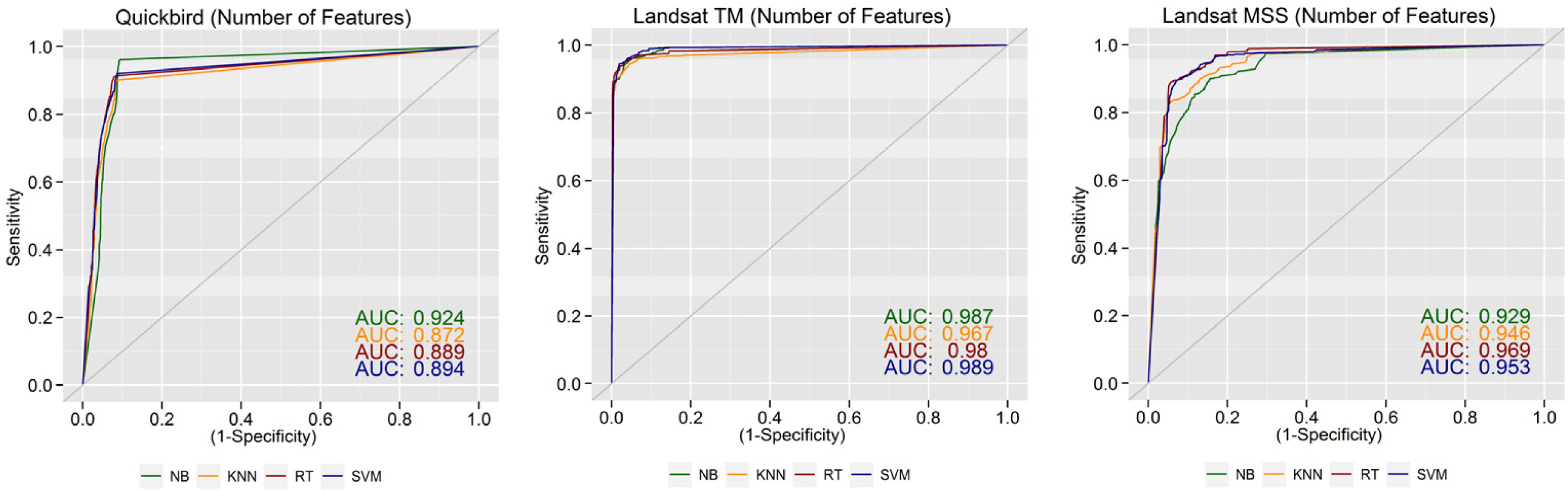
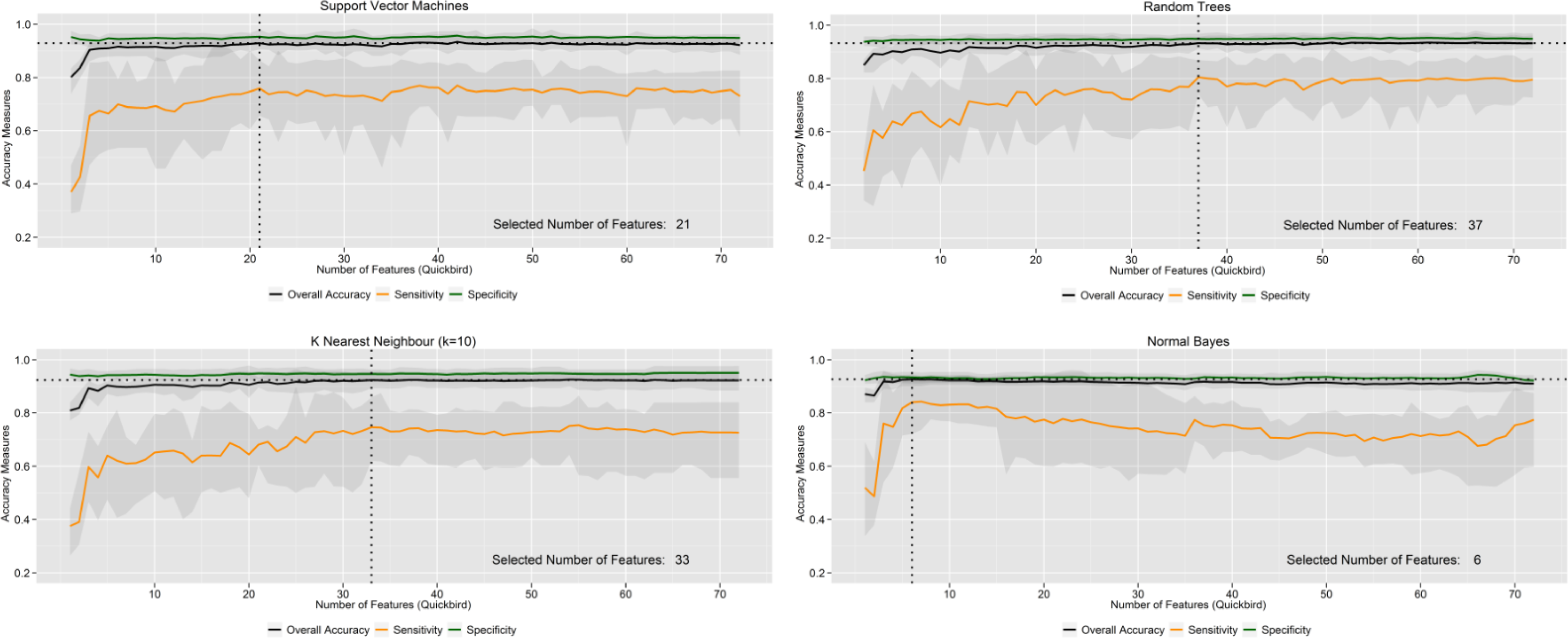
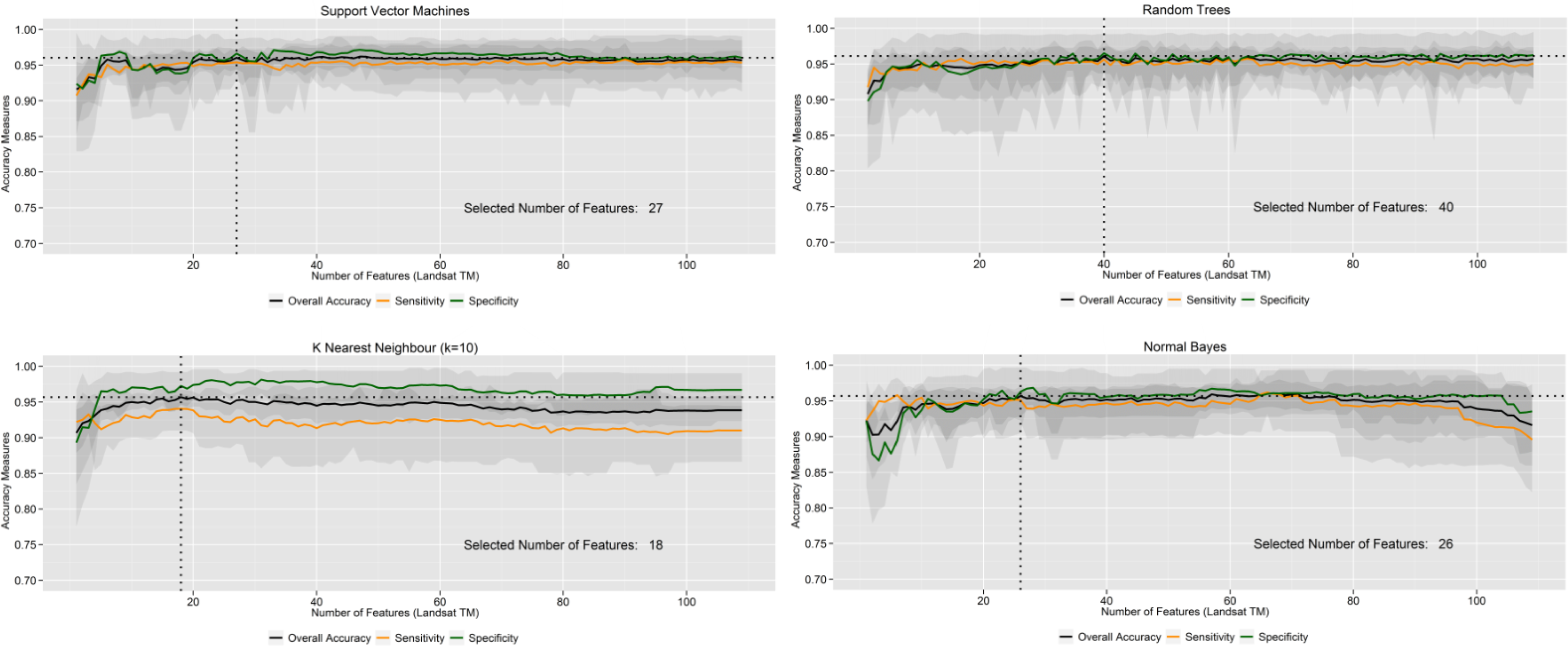
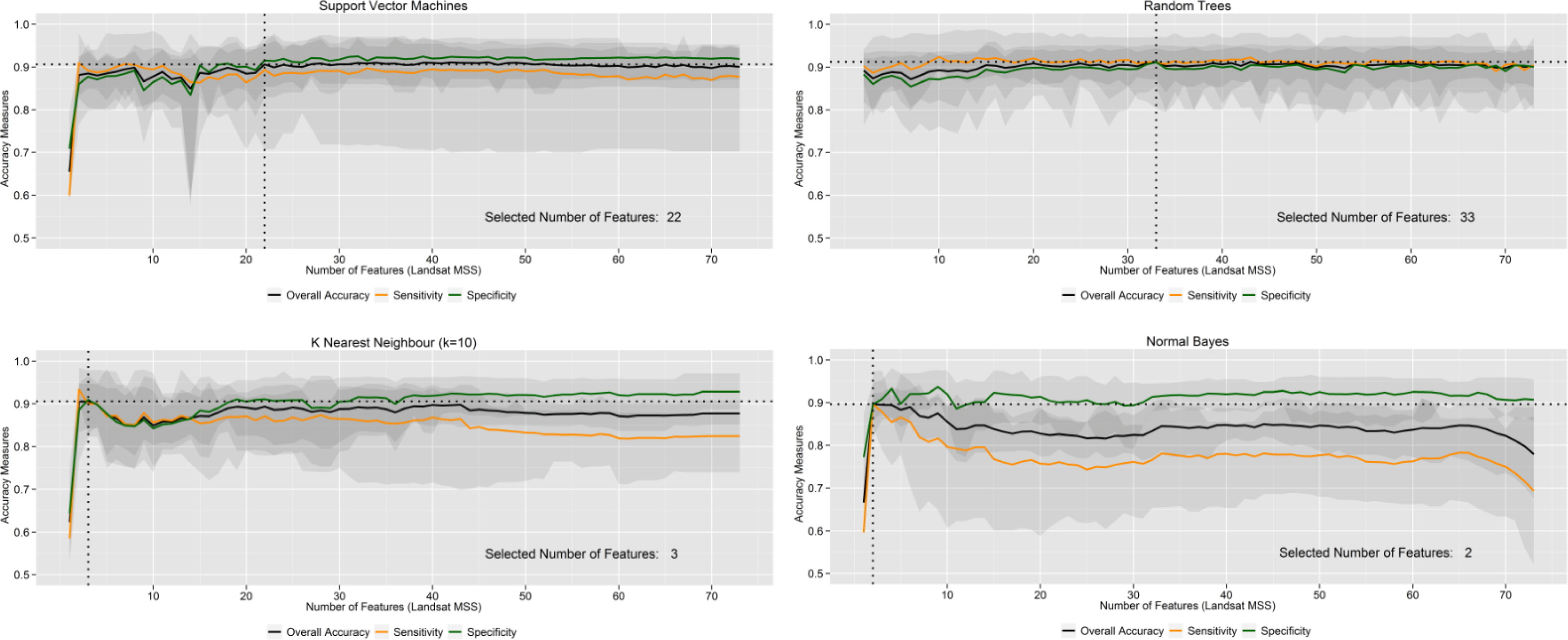
5.2. How Sensitive are Learning Machines to the Size of the Feature Vector?

The performance of machine learning systems, which includes classification accuracy, generalization ability, computational efficiency and learning convergence, can be negatively affected by a failure of the system to discard irrelevant or redundant features [43]. In practice, every classifier deals differently with the dimensionality of the feature space and the decision as to which features to keep and which to discard may vary drastically, depending on the choice of the classifier and the structure of the input data. Therefore, the following experiment aims at choosing for any given classifier and image type a reduced number of features that are relevant and concise enough to achieve high classification accuracies while keeping the computation times short. Given are ten unique (stratified randomly sampled) training datasets for each image type with a size of 1400 (QB), 1200 (TM) or 720 (MSS) instances. Each instance has a maximum dimensionality of 72 (QB), 109 (TM) or 73 (MSS) features and is labeled with one out of five (QB) or three (TM and MSS) classes. For the classification accuracy assessment, the classes are clustered into two groups (“built-up areas” and “not built-up areas”). The feature vector for each image type has been ordered following the outcomes of the ReliefF feature importance ranking. The goal is to test, in a cross-validation on ten unique and stratified randomly sampled testing datasets for each image type (with 350 instances for QB, 300 instances for TM and 280 instances for MSS), the performance and consistency of a classifier while the number of features is iteratively increased along the ranked feature vector. For each classifier, the feature subset that produces the highest average accuracies with the least number of features is selected.

From Figure 3, it can be seen that all classifiers show a good overall performance on the different image types while the size of the feature vector is varied. Figures 4 and 6 show the results for the different classifiers and indicate that for each combination of classifier and image type, there exists an optimal operating point where classification accuracies are maximized while the size of the feature vector is minimal. In the case of the SVM and RT classifiers, shifting the operating point from the optimum by adding more features does not significantly change the resulting accuracies and the classification performance stabilizes with the increasing dimensionality of the feature space. For KNN and NB, the classification accuracies decrease from the optimal operating point as the dimensionality is further increased. This effect is generally known as the Hughes phenomenon [44]. For SVM, the optimal feature subset identified for the recognition of “built-up areas” consists of the first 21 features of the ranked feature vector for QB, the first 27 features for TM and the first 22 features for MSS (Figure 2). For the other classifiers, the optimal dimensionality of the feature space could be identified as 37 (QB), 40 (TM) and 33 (MSS) for RT; 33 (QB), 18 (TM) and 3 (MSS) for KNN; and 6 (QB), 26 (TM) and 2 (MSS) for NB. Averaged over all image types, NB (11) requires the least number of input features to achieve high classification accuracies. KNN (18), SVM (23) and RT (36) need more features to achieve similarly high accuracy values. Even though KNN and NB outperform SVM and RT in terms of the minimum size of the feature vector needed to achieve maximum accuracy values, the undesirable Hughes phenomenon becomes evident for KNN and NB on all image types. With respect to KNN and NB, SVM and RT show stable classification performance with increasing dimensionality of the feature space once the optimal operating point is reached.

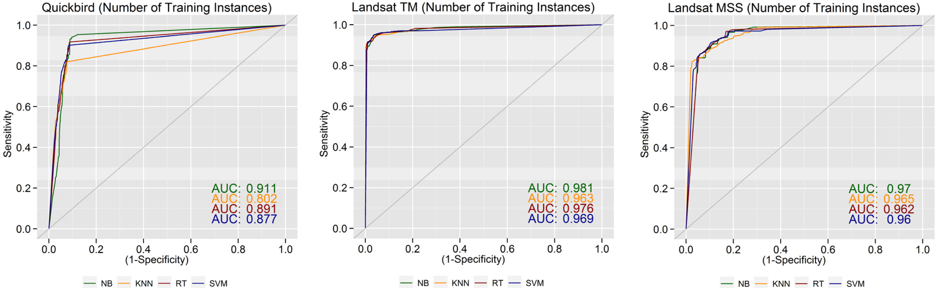
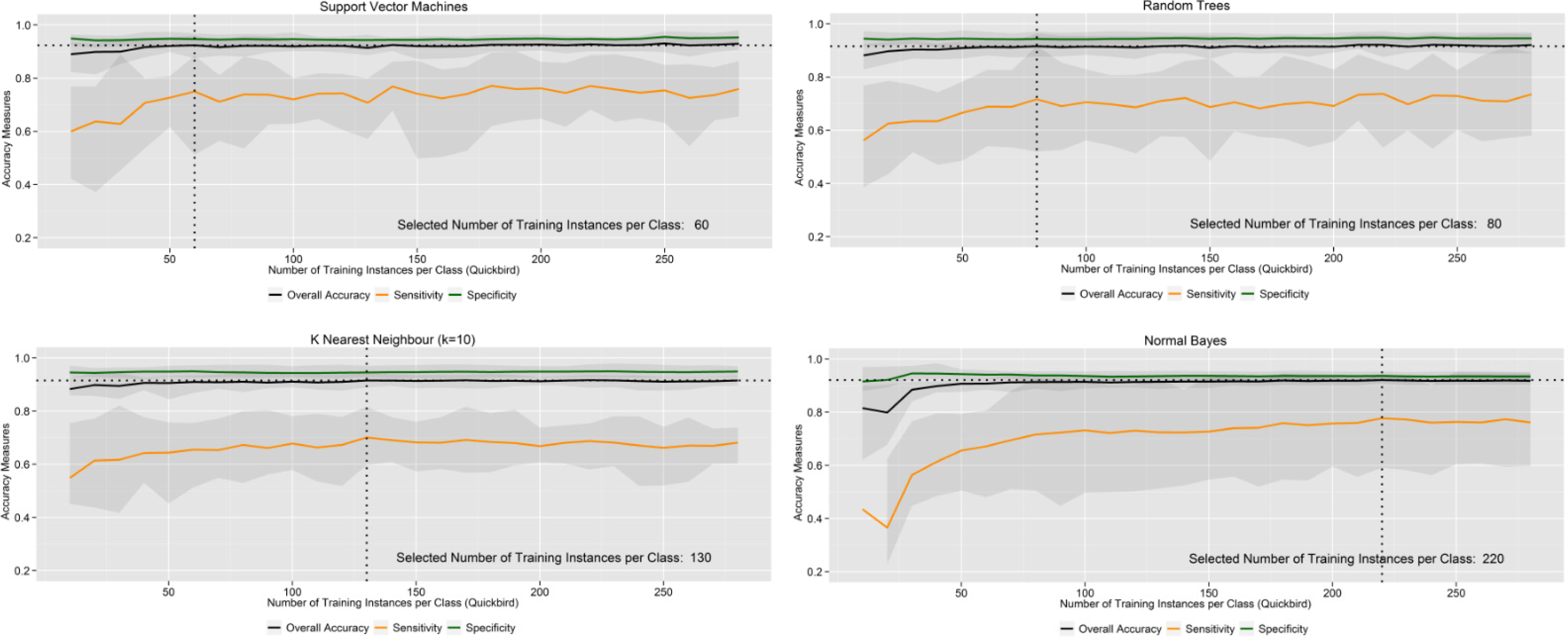
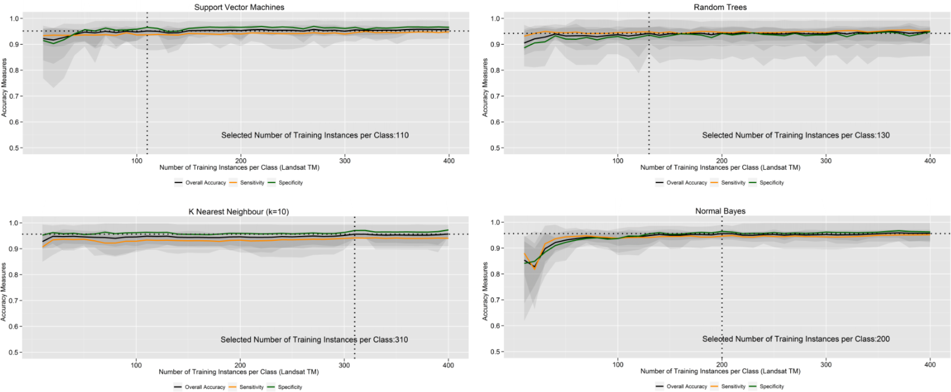
5.3. How does the Number of Training Instances Influence the Performance of the Learning Machines?

The dimensionality of the feature space influences the size of the training data to be captured in that the number of training instances per class should be significantly larger than the number of features. A ratio of at least ten times more training instances than features is recommended in the literature [14]. The following experiment aims at finding for each classifier the minimum number of training instances that is needed to produce stable and high average accuracy values. A similar experimental set up as described in Subsection 5.2 is used with the ten unique training datasets for each image type. The size of the feature vector has been adjusted for each classifier and image type individually based on the results of the experiments described in Subsection 5.2. The goal is to test the performance and consistency of the classifiers while the number of training instances per class is iteratively increased.

From Figure 7, it can be seen that all classifiers show a good overall performance on the different image types while the number of training instances is varied. Besides the slightly poorer performance of KNN on the QB dataset, the classifiers perform comparably well. Figures 8 and 10 show, however, that for each combination of classifier and image type an operating point exists where classification accuracies are maximized while the number of training instances is minimal. Using a smaller number of training instances than is defined at this operating point negatively affects the classification accuracies, whereas an increase in the number of training instances beyond this operating point flattens out the variations in the accuracy values and leads to generally high average accuracies for all classifiers on all datasets. The position of the optimal operating point and therefore the minimum number of instances needed to train a powerful classifier varies between the different learning algorithms and input image types. SVM, when trained on the QB dataset, needs the least number of training instances (60 instances per class) to perform well. RT needs just slightly more instances (80 instances per class), whereas KNN (130 instances per class) and NB (220 instances per class) need significantly more to reach comparable accuracy values. For the TM dataset, SVM needs at least 110, RT 130, KNN 310 and NB 200 instances per class to reach the optimal operating point. When applied to the MSS dataset, SVM should be trained with at least 130, RT with 150, KNN with 230, and NB with 120 instances per class. Averaged over all image types, SVM needs the least number of training instances per class (80), followed by RT (120), KNN (127) and NB (162).

5.4. How well can a Trained Model be Transferred between Different Image Types and Image Scenes?

Table 1 shows the properties of different VHR and MR image types. Despite differences in spatial resolution, it can be seen that there is a clear superimposition of the spectral resolution between the different VHR and MR image types, respectively. Since the feature vectors derived for different image types indicate that the most important features for classification of “built-up areas” are of the spectral and textural domain, it should be possible to transfer a trained classifier from one image type to another, given that spatial and spectral resolution of the image types are in a comparable range. The goal of the following experiments is therefore to evaluate the performance of a classifier when trained on one image type and applied to another.

In a first experiment, the transferability between different VHR image types (QB, WV2 and IK) is evaluated. From the manually labeled reference datasets, ten unique training (1400 instances) and testing (350 instances) datasets have been randomly sampled for each image type. The number of training instances has been chosen based on the results of the experiment described in Subsection 5.3. and has been set large enough to not cause a negative influence on the performance of any of the tested classifiers. The size of the feature vector has been adjusted for each classifier individually based on the results of the experiment described in Subsection 5.2. Therefore, each instance has a dimensionality of 21 features for SVM, 37 features for RT, 33 features for KNN and 6 features for NB. The actual experiment iteratively trains a classifier on one image and tests it on the others. Only comparable spectral bands between the different image types have been used in order to compose identical feature vectors and to allow a transfer of trained learning machines. Figure 11 shows the performance of the classification algorithms for different training-testing scenarios on VHR image types.

The same experiment has also been carried out for MR image types (TM and ETM). Ten unique training (1200 instances) and testing (300 instances) datasets have been randomly sampled for each image type from the reference datasets. Each instance has a dimensionality of 27 features for SVM, 40 features for RT, 18 features for KNN and 26 features for NB. The number of training instances and size of feature vectors have been adjusted based on the results of the experiments described in Subsections 5.2 and 5.3. Figure 12 shows the results for the different classifiers tested on the MR images.

For the VHR image types, all classifiers show an overall good performance when trained and tested on the same image type. The best overall performance for all classifiers can be observed on the WV2 image (Figure 11, WV2WV2). On the IK (Figure 11, IKIK) and QB (Figure 11, QBQB) datasets, KNN performs slightly worse than the others. Trained on IK and applied to QB (Figure 11, IKQB), SVM shows a stable performance, RT performs slightly worse, KNN experiences even a slight performance improvement, and NB shows almost random classification behavior. Applying the same trained models to WV2 (Figure 11, IKWV2) leads to a comparable behavior of NB, SVM and RT, with RT showing even improved performance with respect to the image it has been trained on, while a performance decrease can be observed for KNN. When trained on QB and tested on IK (Figure 11, QBIK), SVM and RT show comparable performance with respect to when they are trained and tested on the same image type. Tested on WV2 (Figure 11, QBWV2), both learning machines show a performance increase. KNN shows a performance increase on both the IK and the WV2 image. NB shows a significant decrease in performance when transferred to other image types with almost a random classification performance on the WV2 test image. Training on the WV2 image and testing on IK (Figure 11, WV2IK), all learning machines, except SVM, experience a significant performance decrease with respect to the image used to train them. QB (Figure 11, WV2QB) shows comparable behavior of SVM, RT and KNN, however, with a significant decrease in accuracy. Tests of NB on the QB image show similar results as for the WV2 image on which it had been trained. Using the range R of the Area Under the Curve (AUC), calculated for each classifier over all VHR image types, as a measure of transferability, SVM (R=0.226) appears to be the best performing classifier in terms of transferability, followed by RT (0.243), KNN (0.311) and NB (0.793).

In addition, for the MR image types, a generally high performance can be observed for all classifiers when trained and tested on the same image type. The best overall performance for all classifiers can be observed for the TM dataset (Figure 12, TMTM). For the ETM dataset (Figure 12, ETMETM), SVM and RT perform best, followed by NB and KNN. However, when trained on TM and tested on ETM (Figure 12, TMETM), a significant performance decrease appears for all classifiers. SVM, RT and KNN still perform well, whereas NB shows the worst performance when transferred. In addition, models trained on ETM and applied to TM (Figure 12, ETMTM) show a decrease in performance for all the classifiers. Nevertheless, SVM, KNN and RT still perform reasonably well, whereas NB shows almost random classification behavior. The range R of the Area Under the Curve (AUC) for each classifier identifies SVM (R=0.143) as best performing classifier in terms of transferability also for MR images, followed by KNN (0.148), RT (0.249) and NB (0.338).

5.5. How does Image Segmentation Influence the Classification Results?

To test the performance of the classifiers with respect to variations in the image segmentation and to evaluate the influence of the segmentation stage on the succeeding object-based classifications, the following experiment was set up. The classifiers are trained and tested on the reference datasets with parameters being tuned according to the outcomes of the experiments described in Sections 5.2 and 5.3. The trained learning machines are applied to a total of 26 segmentations of the same image they were trained on, resulting in 260 classifications per image type when using a 10-fold cross-validation. Segmentation parameters were iteratively varied in order to produce segmentations with increasing average segment size.

Figures 13 and 16 show the results for the different classifiers tested on the QB, TM and MSS images. From Figure 13 a good performance of all classifiers can be observed over all segmentations. Only NB seems to be strongly affected by changes in the segmentation prior to classification, especially on the TM and MSS datasets. The highlighted operating points in Figures 14 and 16 identify the segmentation parameter combinations that were used to produce the segments for the reference datasets. These combinations were identified independently based on the segmentation quality assessments described in Section 3. For all the classifiers on all the image types the optimal segmentation parameters coincides with the operating point of best classification performance. It can also be seen that parameter combinations beyond the identified operating point, which produce segmentations with larger average segment size, negatively affect the classification performance. In addition, a smaller average segment size negatively affects the classification results. This effect becomes more prominent with NB than with SVM, RT and KNN, indicating a lower sensitivity of the latter to the segmentation stage. In addition, the stronger fluctuations of the NB accuracies, especially on the QB and MSS datasets, indicate this performance difference between the classifiers.

6. Discussion

An extended set of spectral, textural and geometrical features has been implemented and tested within this study for the task of urban pattern recognition from multi-spectral satellite images. For the tested scenarios, spectral and textural features showed the highest importance when distinguishing “built-up areas” from “not built-up areas”. Geometrical features deployed a low importance for class separability for the analyzed image types and classification task (Figure 2). For MR image analysis, this was to be expected due to the spatial resolution, whereas for VHR image analysis the result is in contrast to other studies [1]. A possible explanation could be that distinct rectangular shaped building footprints are often partly covered by vegetation in the satellite image and can therefore not adequately be described by geometrical features such as convexity or compactness. However, this should be further investigated with focus on the possible influence of the segmentation and the influence of the specific scene properties. Moreover, the feature set is not exhaustive and implementation of additional features may further constrain the results. NDVI and the mean spectral values of band 4 (NIR) calculated over the segments proved to be important features for all the image types. Particularly interesting is also the importance of TM band 6 (thermal IR) for class separability. As stated in Southworth [45], it has often been ignored in (pixel-based) landcover classification applications, mainly because of its low geometrical resolution (120 m GSD). Given the observation that the average segment size for built-up area recognition in MR satellite images is generally larger than 120 m × 120 m, the lower GSD of the thermal IR band did not negatively influence the geometric outline of the objects of interest, but added additional spectral content when included in the classification of the segments.

For all classifiers and on all image types, an increase in the accuracies could be observed when the number of training instances was increased until an optimal operating point is reached (Figures 8 and 10). A further increase of the training dataset size beyond this operating point does not further improve classification accuracy, but stabilizes it. The optimal operating point, defining the minimum number of training instances needed to train a powerful classifier, varied significantly between the different classifiers and compared with the average number of input features for the classifiers, the best ratio of the number of training instances to features was achieved by RT (3.3) and SVM (3.5). KNN (7.1) and NB (14.7) required significantly more training instances with respect to the size of the feature vector to achieve similar classification accuracies. A possible explanation for why SVM is not strongly affected by changes in the number of training instances and the dimensionality of the feature space, could be that it exploits the concept of margin maximization for classification where adding more training instances may not significantly change the composition of support vectors to span the separating hyperplane. In addition, SVM does not require an estimation of the statistical distribution of classes to perform a classification, as is the case for NB. For standard statistical classifiers like NB, an increase in the dimensionality of the feature space increases the difficulty to estimate from a limited number of training instances the multi-dimensional probability density functions. Therefore, NB is strongly affected by the size of the feature vector and the training dataset.

When trained and tested on the same image type, all classifiers performed comparably well given a large enough training dataset and an optimized size and compilation of the feature vector (Figures 11 and 12). However, when trained on one image type and tested on other image types, large differences with respect to the generalization ability and therefore the transferability could be observed between the different classifiers. SVM showed the best transferability for all VHR and MR image types. RT seemed almost as transferable as SVM, whereas KNN showed a rather unstable behavior when transferred between image types. The worst performance was observed for NB, which showed an almost random classification performance on several image types and clearly lacked generalization ability, indicating the need for a training dataset that closely describes the statistical distribution of the specific image type and image scene to be classified. The results of this experiment showed clear differences in the generalization ability of the different classifiers. However, in order to further strengthen the results, an extended number of image scenes per image type should be considered. Also the effects of techniques to enhance the transferability of classifiers like retraining, domain adaptation or multi-task learning should be evaluated in the context of an object-based image analysis.

Image segmentation clearly affected the succeeding classification stage and optimal operating points for all classifiers coincided with independently assessed optimal segmentation parameter values. SVM, RT and KNN proved to be less sensitive to differences in the segmentation input with respect to NB. Quantitative segmentation accuracy assessment and parameter tuning are therefore important steps to be undertaken when following an object-based image analysis approach, especially when parametric classifiers such as NB are used.

Performance evaluations on the QB image showed for all classifiers comparably low sensitivity values (Figures 4 and 8), which could be an indication that the classification scheme of the reference dataset is not well adjusted. Since a large variety of roof materials is usually present in the built environment, a more refined description of the landuse/landcover class “buildings” depending on the roof material may be a valuable solution to increase the sensitivity of all classifiers. In this context, the generally large variability of spectral signatures within the built environment and regional differences in predominant roof materials may also lead to limitations for the transferability of trained learning machines and should be taken into account when approaching global classification tasks. Using different training datasets between regions that show specific roof material compositions (e.g., tiled roofs in large parts of Central Europe, thatched and metal roofs in rural South East Asia) should be further evaluated especially for the VHR image analysis.

7. Conclusions

This paper described a method for the recognition of urban patterns at different spatial scales in MR and VHR multi-spectral satellite images using machine learning algorithms in the context of a state-of-the-art object-based image analysis. Moving towards a more pattern-oriented approach, which effectively makes use of image domains beyond the spectral content on the pixel level, proved to be a valuable solution when extracting information on the built environment. Particular emphasis was given to an extensive performance analysis of the classification algorithms under varying conditions in order to optimize their usage and assess their applicability to urban pattern recognition tasks. The actual characteristics of the method, including transferability and stability to changes in image type and algorithm parameters were assessed and a performance evaluation framework with focus on object-based image analysis has been proposed to complement the information provided by commonly used accuracy assessments of the final map product. SVM and RT appeared to be the best performing classifiers on all image types according to the predefined performance requirements. KNN and NB showed good performance in some configurations, but mainly lacked the ability to generalize and showed unstable behavior under varying training-testing scenarios.

Combining quantitative feature selection with machine learning classification algorithms allowed for a high degree of process automation and showed great flexibility regarding transferability of the method to diverse image types and image scenes. In this context, also segmentation parameter tuning proved to be an important step in an object-based image analysis. In comparison to widely used expert systems based on fuzzy set theory, local expert knowledge can be integrated easily into the processing flow by training data selection for which a user does not necessarily need to have detailed knowledge of remote sensing image analysis. Moreover, the use of machine learning allows for easy adjustment and transfer of the method not only to different datasets coming from past and present satellite missions, but also to datasets from upcoming future space-borne missions such as the Sentinel-2 super-spectral satellite of the European Space Agency (ESA) [46] or Digital Globe’s WorldView-3 VHR satellite. Performance analysis and algorithm optimization to the lately released Landsat-8 super-spectral MR imagery are currently on going.

The results of this study indicate great potential of the implemented classification and performance evaluation framework to be integrated into an automated processing chain from data acquisition to user-ready built-up area products. A real-world application of the SVM algorithm, optimized and trained within this study for built-up area recognition from MR and VHR images, can be found in Wieland, et al. [47]. The study uses multi-source imaging to assess an exposed building stock and its population as input for a probabilistic seismic vulnerability assessment [48]. The proposed method for training and optimizing classifiers has also successfully been applied to the recognition of more refined urban patterns which outline areas of predominant building types from Landsat TM data, as is described in Wieland et al. [49] and Tyagunov et al. [50]. Future work will focus on assessing the feasibility of developing an automated processing chain to derive urban information products from multi-spectral satellite images at multiple scales with large (regional or global) coverage.

References

1. Blaschke, T. Object based image analysis for remote sensing. ISPRS J. Photogramm. Remote Sens 2010, 65, 2–16. [Google Scholar]
2. Yan, G.; Mas, J.F.; Maathuis, B.H.P.; Zhang, X.; van Dijk, P.M. Comparison of pixel-based and object-oriented image classification approaches: A case study in a coal fire area, Wuda, Inner Mongolia, China. Int. J. Remote Sens 2006, 27, 4039–4055. [Google Scholar]
3. Taubenböck, H.; Roth, A. A Transferable and Stable Object Oriented Classification Approach in Various Urban Areas and Various High Resolution Sensors. In Proceedings of the Joint Urban Remote Sensing Event, Paris, France, 11–13 March 2007; pp. 1–7.
4. Weng, Q. Remote sensing of impervious surfaces in the urban areas: Requirements, methods, and trends. Remote Sens. Environ 2012, 117, 34–49. [Google Scholar]
5. Schneider, A. Monitoring land cover change in urban and peri-urban areas using dense time stacks of Landsat satellite data and a data mining approach. Remote Sens. Environ 2012, 124, 689–704. [Google Scholar]
6. Zhang, Q.; Wang, J.; Peng, X.; Gong, P.; Shi, P. Urban built-up land change detection with road density and spectral information from multi-temporal Landsat TM data. Int. J. Remote Sens 2002, 23, 3057–3078. [Google Scholar]
7. Lillesand, T.M.; Kiefer, R.W.; Chipman, J.W. Remote Sensing and Image Interpretation; John Wiley & Sons: New York, NY, USA, 2008. [Google Scholar]
8. Haralick, R.; Shanmugam, K.; Dinstein, I. Textural features for image classification. IEEE Trans. Sys. Man Cyber 1973, 3, 610–621. [Google Scholar]
9. Van der Werff, H.M.A.; van der Meer, F.D. Shape-based classification of spectrally identical objects. ISPRS J. Photogramm. Remote Sens 2008, 63, 251–258. [Google Scholar]
10. Hu, M.K. Visual pattern recognition by moment invariants. IRE Trans. Inf. Theory 1962, 8, 179–187. [Google Scholar]
11. Zhang, D.; Lu, G. Review of shape representation and description techniques. Pattern Recognit 2004, 37, 1–19. [Google Scholar]
12. Peura, M; Iivarinen, J. Efficiency of simple shape descriptors. Asp. Vis. Form 1997, 443–451. [Google Scholar]
13. Langley, P. Selection of Relevant Features in Machine Learning. In Proceedings of the AAAI Fall Symposium, New Orleans, LA, USA, 4–6 November 1994; pp. 127–131.
14. Koprinska, I. Feature Selection for Brain-Computer Interfaces. In Proceedings of the 13th Pacific-Asia International Conference on Knowledge Discovery and Data Mining: New Frontiers in Applied Data Mining, Bangkok, Thailand, 27–30 April 2009; pp. 106–117.
15. Witten, I.H.; Frank, E.; Hall, M.A. Data Mining: Practical Machine Learning Tools and Techniques; Elsevier: Amsterdam, The Netherlands, 2011. [Google Scholar]
16. Novack, T.; Esch, T.; Kux, H.; Stilla, U. Machine learning comparison between WorldView-2 and QuickBird-2-simulated imagery regarding object-based urban land cover classification. Remote Sens 2011, 3, 2263–2282. [Google Scholar]
17. Prandi, F.; Brumana, R.; Fassi, F. Semi-automatic objects recognition in urban areas based on fuzzy logic. J. Geogr. Inf. Syst 2010, 2, 55–62. [Google Scholar]
18. Benz, U.C.; Hofmann, P.; Willhauck, G.; Lingenfelder, I.; Heynen, M. Multi-resolution, object-oriented fuzzy analysis of remote sensing data for GIS-ready information. ISPRS J. Photogramm. Remote Sens 2004, 58, 239–258. [Google Scholar]
19. Tzotsos, A.; Argialas, D. A. Support Vector Machine Approach for Object Based Image Analysis. In Proceedings of 1st International Conference on Object-based Image Analysis, Salzburg, Austria, 4–5 July 2006.
20. Bruzzone, L.; Marconcini, M. Toward the Automatic Updating of Land-Cover Maps by a Domain-Adaptation SVM Classifier and a Circular Validation Strategy. IEEE Trans. Geosci. Remote Sens 2009, 47, 1108–1122. [Google Scholar]
21. Bruzzone, L.; Prieto, D.F. Unsupervised retraining of a maximum likelihood classifier for the analysis of multitemporal remote sensing images. IEEE Trans. Geosci. Remote Sens 2001, 39, 456–460. [Google Scholar]
22. Leiva-Murillo, J.M.; Gómez-Chova, L.; Camps-Valls, G. Multitask remote sensing data classification. IEEE Trans. Geosci. Remote Sens 2013, 51, 151–161. [Google Scholar]
23. Parker, J.A.; Kenyon, R.V.; Troxel, D.E. Comparison of interpolating methods for image resampling. IEEE Trans. Med. Imaging 1983, 2, 31–39. [Google Scholar]
24. Neteler, M.; Mitasova, H. Open Source GIS: A Grass GIS Approach; Springer: Heidelberg, Germany, 2002. [Google Scholar]
25. Pohl, C.; van Genderen, J.L. Multisensor image fusion in remote sensing: Concepts, methods and applications. Int. J. Remote Sens 1998, 19, 823–854. [Google Scholar]
26. Felzenszwalb, P.; Huttenlocher, D. Efficient graph-based image segmentation. Int. J. Comput. Vis 2004, 59, 167–181. [Google Scholar]
27. ISPRS Data Sets: Ikonos. 2003. Available online: http://www.isprs.org/data/ikonos (accessed on 8 April 2013).
28. Clinton, N.; Holt, A.; Scarborough, J.; Yan, L.; Gong, P. Accuracy assessment measures for object-based image segmentation goodness. Photogramm. Engine. Remote Sens 2010, 76, 289–299. [Google Scholar]
29. Zhang, H.; Fritts, J.E.; Goldman, S.A. Image segmentation evaluation: a survey of unsupervised methods. Computerv. Image Underst 2008, 110, 260–280. [Google Scholar]
30. Johnson, B.; Xie, Z. Unsupervised image segmentation evaluation and refinement using a multi-scale approach. ISPRS J. Photogramm. Remote Sens 2011, 66, 473–483. [Google Scholar]
31. Bradski, G.; Kaehler, A. Learning OpenCV; O’Reilly: Sebastopol, CA, USA, 2008. [Google Scholar]
32. Fukunaga, K. Introduction to Statistical Pattern Recognition; Elsevier: Amsterdam, The Netherlands, 1990. [Google Scholar]
33. Wu, X.; Kumar, V.; Ross Quinlan, J.; Ghosh, J.; Yang, Q.; Motoda, H.; McLachlan, G.J.; Ng, A.; Liu, B.; Yu, P.S.; et al. Top 10 algorithms in data mining. Knowl. Inf. Syst 2007, 14, 1–37. [Google Scholar]
34. Breiman, L. Random forests. Mach. Learn 2001, 45, 5–32. [Google Scholar]
35. Breiman, L.; Cutler, A. Random forests. Available online: http://www.stat.berkeley.edu/users/breiman/RandomForests (accessed on 07 March 2013).
36. Pal, M.; Mather, P.M. An assessment of the effectiveness of decision tree methods for land cover classification. Remote Sens. Environ 2003, 86, 554–565. [Google Scholar]
37. Vapnik, V. The Nature of Statistical Learning Theory; Springer: New York, NY, USA, 2000. [Google Scholar]
38. Burges, C.J. A tutorial on support vector machines for pattern recognition. Data Mini. Knowl. Discov 1998, 2, 121–167. [Google Scholar]
39. Yang, H.; Ma, B.; Du, Q.; Yang, C. Improving urban land use and land cover classification from high-spatial-resolution hyperspectral imagery using contextual information. J. Appl. Remote Sens 2010. [Google Scholar] [CrossRef]
40. Kononenko, I. Estimating Attributes: Analysis and Extensions of Relief. In Proceedings of the International Conference on Machine Learning, New Brunswick, NJ, USA, 10–13 July 1994; pp. 171–182.
41. WEKA3: Data Mining with Open Source Machine Learning Software. 2012. Available online: http://www.cs.waikato.ac.nz/ml/weka (accessed on 29 October 2012).
42. Robnik-Sikonja, M.; Kononenko, I. Theoretical and empirical analysis of ReliefF and RReliefF. Mach Learn 2003, 53, 23–69. [Google Scholar]
43. Nguyen, M.H.; De la Torre, F. Optimal feature selection for support vector machines. Pattern Recognit 2010, 43, 584–591. [Google Scholar]
44. Hughes, G. On the mean accuracy of statistical pattern recognizers. IEEE Trans. Inf. Theory 1968, 14, 55–63. [Google Scholar]
45. Southworth, J. An assessment of Landsat TM band 6 thermal data for analyzing land cover in tropical dry forest regions. Int. J. Remote Sens 2004, 25, 689–706. [Google Scholar]
46. Martimor, P.; Arino, O.; Berger, M.; Biasutti, R.; Carnicero, B.; Del Bello, U.; Fernandez, V.; Gascon, F.; Silvestrin, P.; Spoto, F.; et al. Sentinel-2 Optical High Resolution Mission for GMES Operational Services. In Proceedings of the IEEE International Geoscience and Remote Sensing Symposium, Barcelona, Spain, 23–28 July 2007; pp. 2677–2680.
47. Wieland, M.; Pittore, M.; Parolai, S.; Zschau, J. Exposure estimation from multi-resolution optical satellite imagery for seismic risk assessment. ISPRS Int. J. Geo-Inf 2012, 1, 69–88. [Google Scholar]
48. Pittore, M.; Wieland, M. Toward a rapid probabilistic seismic vulnerability assessment using satellite and ground-based remote sensing. Nat. Hazards 2013, 68, 115–145. [Google Scholar]
49. Wieland, M.; Pittore, M.; Parolai, S.; Zschau, J.; Moldobekov, B.; Begaliev, U. Estimating building inventory for rapid seismic vulnerability assessment: Towards an integrated approach based on multi-source imaging. Soil Dyn. Earthq. Eng 2012, 36, 70–83. [Google Scholar]
50. Tyagunov, S.; Pittore, M.; Wieland, M.; Parolai, S.; Bindi, D.; Fleming, K.; Zschau, J. Uncertainty and sensitivity analyses in seismic risk assessments on the example of Cologne, Germany. Nat. Hazards Earth Syst. Sci. Discuss 2014, 1, 7285–7332. [Google Scholar]
Figure 1. (a) Image subsets. (b) Image segmentations. (c) Reference datasets.
Remotesensing 06 02912f1aRemotesensing 06 02912f1b
Figure 2. Features for the Landsat Thematic Mapper (TM), Landsat Multi-Spectral Scanner (MSS) and Quickbird (QB) reference dataset grouped into spectral, textural and geometrical features and ranked by their importance for distinguishing built-up from not built-up areas. For each image type, the ten most important features are highlighted. A description of the features can be found in Tables 2 and 3.
Remotesensing 06 02912f2
Figure 3. ROC curves for the classification of QB, TM and MSS, depicting the performance of different classifiers under varying sizes of the feature vector.
Remotesensing 06 02912f3
Figure 4. Influence of the size of the feature vector on the classification accuracy for QB. Mean and range of accuracy measures from the ten-fold cross-validation are shown for each iteration.
Remotesensing 06 02912f4
Figure 5. Influence of the size of the feature vector on the classification accuracy for TM. Mean and range of accuracy measures from the ten-fold cross-validation are shown for each iteration.
Remotesensing 06 02912f5
Figure 6. Influence of the size of the feature vector on the classification accuracy for MSS. Mean and range of accuracy measures from the ten-fold cross-validation are shown for each iteration.
Remotesensing 06 02912f6
Figure 7. ROC curves for the classification of QB, TM and MSS, depicting the performance of different classifiers under varying numbers of training instances.
Remotesensing 06 02912f7
Figure 8. Influence of the training set size on the classification accuracy for QB. Mean and range of accuracy measures from the ten-fold cross-validation are shown for each iteration.
Remotesensing 06 02912f8
Figure 9. Influence of the training set size on the classification accuracy for TM. Mean and range of accuracy measures from the ten-fold cross-validation are shown for each iteration.
Remotesensing 06 02912f9
Figure 10. Influence of the training set size on the classification accuracy for MSS. Mean and range of accuracy measures from the ten-fold cross-validation are shown for each iteration.
Remotesensing 06 02912f10
Figure 11. Classifier performance for different training-testing scenarios on VHR image types.
Remotesensing 06 02912f11
Figure 12. Classifier performance for different training-testing scenarios on MR image types.
Remotesensing 06 02912f12
Figure 13. ROC curves for the classification of QB, TM and MSS, depicting the performance of different classifiers under varying segmentation inputs.
Remotesensing 06 02912f13
Figure 14. Influence of the segmentation inputs on the classification accuracy for QB with increasing average segment size from left to right. Mean and range of accuracy measures from the ten-fold cross-validation are shown for each iteration.
Remotesensing 06 02912f14
Figure 15. Influence of the segmentation inputs on the classification accuracy for TM with increasing average segment size from left to right. Mean and range of accuracy measures from the ten-fold cross-validation are shown for each iteration.
Remotesensing 06 02912f15
Figure 16. Influence of the segmentation inputs on the classification accuracy for MSS with increasing average segment size from left to right. Mean and range of accuracy measures from the ten-fold cross-validation are shown for each iteration.
Remotesensing 06 02912f16