Automatic Orientation of Multi-Scale Terrestrial Images for 3D Reconstruction

Abstract

Image orientation requires ground control as a source of information for both indirect estimation and quality assessment to guarantee the accuracy of the photogrammetric processes. However, the orientation still depends on interactive measurements to locate the control entities over the images. This paper presents an automatic technique used to generate 3D control points from vertical panoramic terrestrial images. The technique uses a special target attached to a GPS receiver and panoramic images acquired in nadir view from different heights. The reference target is used as ground control to determine the exterior orientation parameters (EOPs) of the vertical images. These acquired multi-scale images overlap in the central region and can be used to compute ground coordinates using photogrammetric intersection. Experiments were conducted in a terrestrial calibration field to assess the geometry provided by the reference target and the quality of the reconstructed object coordinates. The analysis was based on the checkpoints, and the resulting discrepancies in the object space were less than 2 cm in the studied cases. As a result, small models and ortho-images can be produced as well as georeferenced image chips that can be used as high-quality control information.

1. Introduction

Despite advances in direct sensor orientation (DSO), ground control remains essential in remote sensing and photogrammetric processes with a large variety of applications that require ground control points (GCPs) in their procedures. Examples of the relevance of ground control in the field of remote sensing are briefly discussed here. Dandois and Ellis [1] extracted 3D point clouds from high-spatial-resolution kit photographs using bundle adjustment. The GCPs were extracted interactively from existing high-resolution ortho-photographs to transform the generated point cloud into a cartographic plane projection system (Universal Transverse Mercator—UTM). The authors argued that it was not feasible to identify each keypoint extracted from the aerial photographs in the ortho-photographs, and to circumvent this limitation, they used averages of sets of keypoints near each GCP. As shown later in this paper, the proposed approach eliminates this type of limitation. Wondie et al. [2] generated spatiotemporal information from satellite images on land-cover dynamics for biodiversity management. To achieve this goal, the authors used GCPs to georeference the satellite images and also acquired photographs to document the reference areas. Nakano and Chikatsu [3] created a 3D measurement system for various applications in close range environments, which was calibrated using only distances and pseudo-GCPs. To assess the accuracy of the system in a real application, the authors used checkpoints measured in the field with a total station. Harwing and Lucieer [4] presented an assessment of the accuracy achieved in 3D point clouds generated from images acquired by an optical camera on board unmanned aerial vehicles (UAVs) and processed with multi-view stereopsis (MVS) techniques. The authors compared the point clouds generated via a photogrammetric technique with the GCPs surveyed using a procedure that combines total station and differential GPS (DGPS) data. Tommaselli et al. [5] developed a technique to generate virtual aerial images from oblique frames in which the GCPs were located interactively. In all of these studies, GCPs were required as a component of the algorithm to assess the results or to correct systematic errors.

There have been many efforts to fully automate the process of acquisition, calibration, and orientation of images to recover the 3D coordinates of geometric features in a scene. In general, one problem that arises involves measuring ground control features and establishing correspondence between a given model of ground control and its corresponding representation extracted from an image.

The photogrammetric measurement process requires the detection, identification, and precise location of imaged control points. Object coordinates must be determined from well-defined features, and both presignalized and natural points are typically used. Presignalized points are widely employed in close-range photogrammetry, and natural points are typically used as the GCPs for aerial triangulation. However, the automatic recognition process becomes complicated if presignalized targets are not used.

Presignalized points are marked on the ground before acquiring the aerial images. The signalization allows the identification and measurement process to be automated, but it has disadvantages due to manufacturing and installation costs and restrictions that must be installed before carrying out the flight.

However, natural points are well-defined elements that are normally available in the project area. As a drawback, natural features are not as distinguishable as presignalized targets and are not always available in suitable regions of the photogrammetric project. Currently, only a few points are required due to the availability of direct georeferencing data, but the measurements of natural points in images are still performed by human operators.

Gülch [6] reported on the main problems in automating the measurement of GCPs. If presignalized points are used, suitable models with respect to size, shape, and background must be designed and the color and contrast of the images must also be considered. Natural points are related to man-made features, i.e., traffic signs on the ground, building corners, land boundary corners, and road intersections. The natural points should be unique and locatable with high precision.

Heipke [7] presented a study on control information for image orientation and several requirements that must be fulfilled to obtain a reliable control source. Ideally, a ground control should offer: Good geometric and radiometric conditions, visibility in different views, scale invariance, distinctness.

Another problem with the location of ground control is accessibility for surveying. Shadowed areas and areas near water should also be avoided.

An additional review was published by Hanh [8] on automatic measurement of GCPs in a study of a semi-automatic process for extraction of signalized points with the conclusion that the technique was successful in certain specific cases; however, a general solution was still missing.

Various types of ground control have already been considered for exterior orientation. Jaw and Wu [9] described important works addressing different control information. Points, lines, areal features, and structural forms were commonly used.

Berveglieri et al. [10] presented a technique used to locate GCPs based on templates generated from panoramic terrestrial images acquired with a telescopic pole and fisheye camera. As originally proposed, this technique uses area-based matching refined with least-squares matching to precisely locate the terrestrial template in the aerial image. Selected problems were not covered in that work, such as the geometric deformations in the template caused by the slope around the GCP.

With respect to the 3D object reconstruction, Remondino and El-Hakim [11] summarized in their paper significant studies concerning modeling from images. The main problems and certain available solutions were described for the generation of 3D models using terrestrial images in close-range photogrammetry. The 3D point determination based on images uses image measurements supported by a mathematical model to recover the position (X, Y, Z) in the object space. Image-based methods obtain 3D coordinates from multiple views and employ projective or a perspective camera model.

Barazzetti et al. [12] developed an automated methodology by combining algorithms and techniques for image-based 3D modeling in close range. The authors oriented images acquired by a calibrated camera and extracted accurate point clouds from the estimated EOPs. Details on 3D reconstruction using optical images can be found in Luhmann et al. [13].

For many years, photogrammetry addressed 3D reconstruction using images and developed efficient commercial packages for this task; however, the location of points still relies on interactive measurements for both the orientation and modeling steps (except for tie points).

In this paper, an alternative approach is introduced for the automatic image orientation and generation of a 3D point cloud in close-range photogrammetry. The objective is to present and to assess an original technique encompassing terrestrial image acquisition, automatic image orientation, and 3D reconstruction of small areas. As a result, high resolution georeferenced images, a small DTM and ortho images can be obtained.

The proposed technique uses a target attached to a global navigation satellite system (GNSS) receiver. During the field survey, terrestrial images of GCP areas are acquired in nadir view in large-scale and at different heights from the same position. A multi-scale photogrammetric model is formed and processed by bundle adjustment. Subsequently, products can be derived, i.e., a point cloud, ortho-image, or georeferenced template for use in the orientation of aerial images.

This survey of a conventional GCP requires no increase in time demand, and only marginal costs are added due to the insertion of a camera and pole. The entire imaging system is mounted and the images are acquired during the survey of a GCP. Wide-angle or fisheye lenses are required to cover large areas around the point, primarily due to the image acquired at the lowest height, which reduces the coverage area. However, these additional devices are common and inexpensive. In addition, this technique removes the dependency on point features. The GNSS receiver can be installed in any area and requires only a few distinguishable features near the receiver, which appear in the images.

A rigorous calibration process using a specific model for a fisheye lens was previously performed to define the camera parameters, and experiments with a bundle adjustment were processed with consideration of the targeted panel as the ground control for the original fisheye and resampled images.

A complete analysis of the results was performed using independent checkpoints. The differences between each estimated 3D point and its true coordinates allowed for an assessment of the discrepancies in the object space. The quality of the object reconstruction was also assessed with respect to the area size and with consideration of the radial effect resulting from the geometry of the reference panel.

The following sections present an explanation of the method developed for the object reconstruction, and the discussion is based on experiments performed in the calibration field. Finally, the paper concludes with a brief summary and recommendations for future work.

2. Automatic Method for 3D Point Determination

The proposed approach performs an automatic flow for the recognition of a square target (Figure 1b), image orientation, and object reconstruction. A bundle adjustment can be processed to generate 3D coordinates of any point in the scene using a set of vertically displaced images. Five steps were identified to describe the method: camera calibration, image acquisition, automatic target detection, generation of a multi-scale model with bundle adjustment, and determination of 3D points.

2.1. Camera Calibration

First, the camera must be calibrated to estimate the interior orientation parameters (IOPs), which are normally the focal length, principal point coordinates, and lens distortion coefficients [14]. In general, the mathematical model uses the collinearity equations and includes the lens distortion parameters (Equation (1)):

$$\begin{array}{l}{F}_1=x_f-x_0+\delta x_r+\delta x_d+\delta x_a+f\frac{m_{11}(X-X_0)+m_{12}(Y-Y_0)+m_{13}(Z-Z_0)}{m_{31}(X-X_0)+m_{32}(Y-Y_0)+m_{33}(Z-Z_0)}\\ F_2=y_f-y_0+\delta y_r+\delta y_d+\delta y_a+f\frac{m_{21}(X-X_0)+m_{22}(Y-Y_0)+m_{23}(Z-Z_0)}{m_{31}(X-X_0)+m_{32}(Y-Y_0)+m_{33}(Z-Z_0)}\end{array}$$

(1)

in which x_f, y_f are the image coordinates, (X, Y, Z) are the coordinates of the same point in the object space, m_ij are the rotation matrix elements, (X₀, Y₀, Z₀) are the coordinates of the camera perspective center (PC), (x₀, y₀) are the principal point coordinates, f is the camera focal length, and δx_i, δy_i are the effects of the radial decentering lens distortion and affinity model, respectively [15].

However, the image acquisition does not follow the collinearity conditions due to the internal geometry of the fisheye lens. The rays are refracted toward the optical axis, and thus, a suitable model should be used. Most of the fisheye lenses are constructed using equidistant projection [16].

The calibration developed for the purposes of this paper uses a conventional bundle adjustment with the equidistant model [16] of Equation (2) and additional parameters of the Conrady-Brown lens distortion model [14].

$$\begin{array}{l}{x}^{\prime }=x_0+\mathrm{\Delta }x-f.\frac{X_C}{\sqrt{X_C^2+Y_C^2}}.\text{arctan}\left(\frac{\sqrt{X_C^2+Y_C^2}}{Z_C}\right)\\ y^{\prime }=y_0+\mathrm{\Delta }y-f.\frac{Y_C}{\sqrt{X_C^2+Y_C^2}}.\text{arctan}\left(\frac{\sqrt{X_C^2+Y_C^2}}{Z_C}\right)\end{array}$$

(2)

in which f is the camera focal length, (X_C, Y_C, Z_C) are the 3D point coordinates in the photogrammetric reference system, (x′, y′) are the image point coordinates in the photogrammetric reference system, (x₀, y₀) are the coordinates of the principal point, and Δx and Δy are the effects of the lens distortion.

Equation (2) can be used to define a system of non-linear redundant equations in which the image coordinates are the observations and the IOPs, EOPs, and object point coordinates are the unknowns. The system can be solved using the least-squares method and considering certain constraints imposed on the ground coordinates, object distances, or EOP observations.

2.2. Image Acquisition

Vertical images are acquired using a technique specially designed to generate multi-scale models of areas with distinct features. The following devices are required to acquire the images, as shown in Figure 1:

The reference panel is a special target composed of a white panel (50 × 50 cm) on which a 6-cm-thich black square (42 × 42 cm) is displayed. The panel is placed under the GNSS antenna receiver on a tripod for leveling. A second tripod with a telescopic pole is positioned at a distance (D) to the side of the GNSS antenna, and a digital camera is installed over this pole pointing downward and raised to previously defined heights, as depicted in Figure 2a.

An image of the surrounding area of the panel is acquired for each height. The square is perpendicularly aligned toward the telescopic pole to define a local coordinate system (X_L, Y_L, Z_L).

The centroid position of the square is determined by the GNSS survey, and the local coordinates can be transformed into geographic coordinates or plane coordinates (E, N, h) if the azimuth of this local reference system is known (e.g., using a compass or second GNSS receiver). Figure 2b illustrates the relationship between the pole axis and the camera’s external nodal point.

To perform the experiments, the devices are installed to collect GNSS signals over a point feature or near distinguishable elements in their neighborhood. While a point is surveyed using the GNSS receiver, three images are collected at different heights (H_i) without changing the position of the telescopic pole. The heights (A_I and H_i) are measured by an EDM or by a graduated rule on the telescopic pole. The relative positions (measured with an EDM or measuring tape) and heights are used to provide initial approximations or observations for the (X_C, Y_C, Z_C) parameters in the image orientation process.

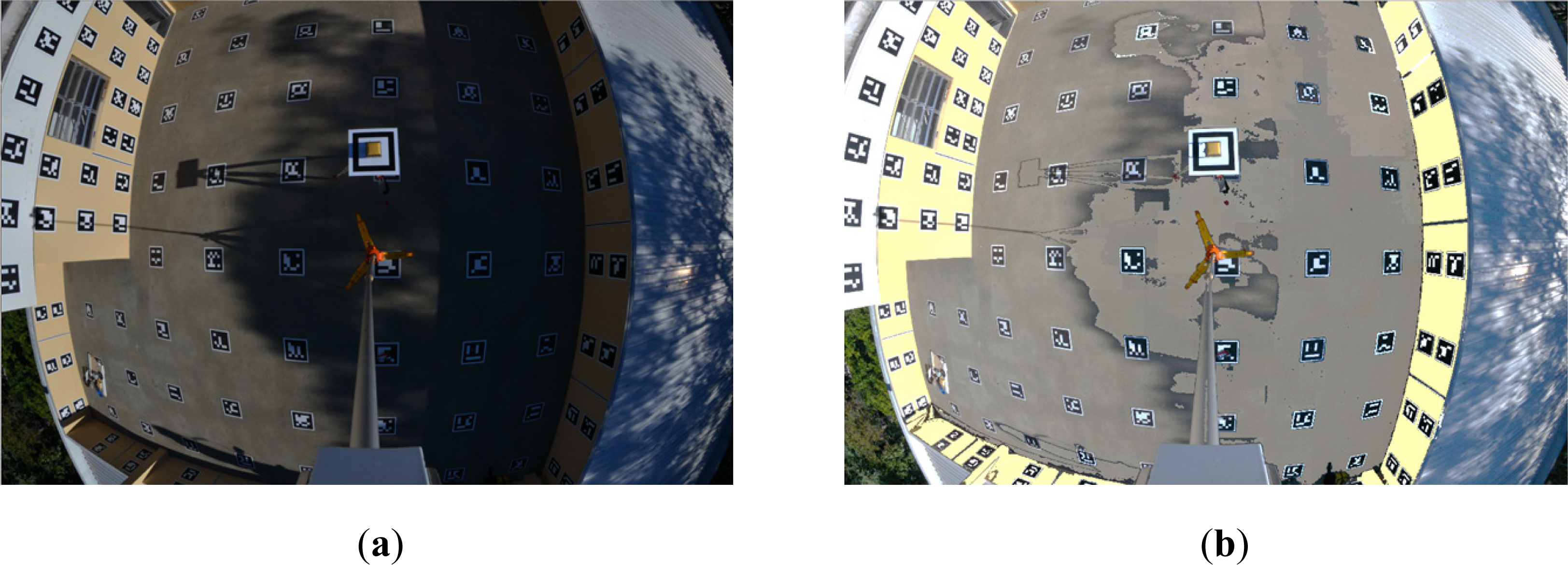
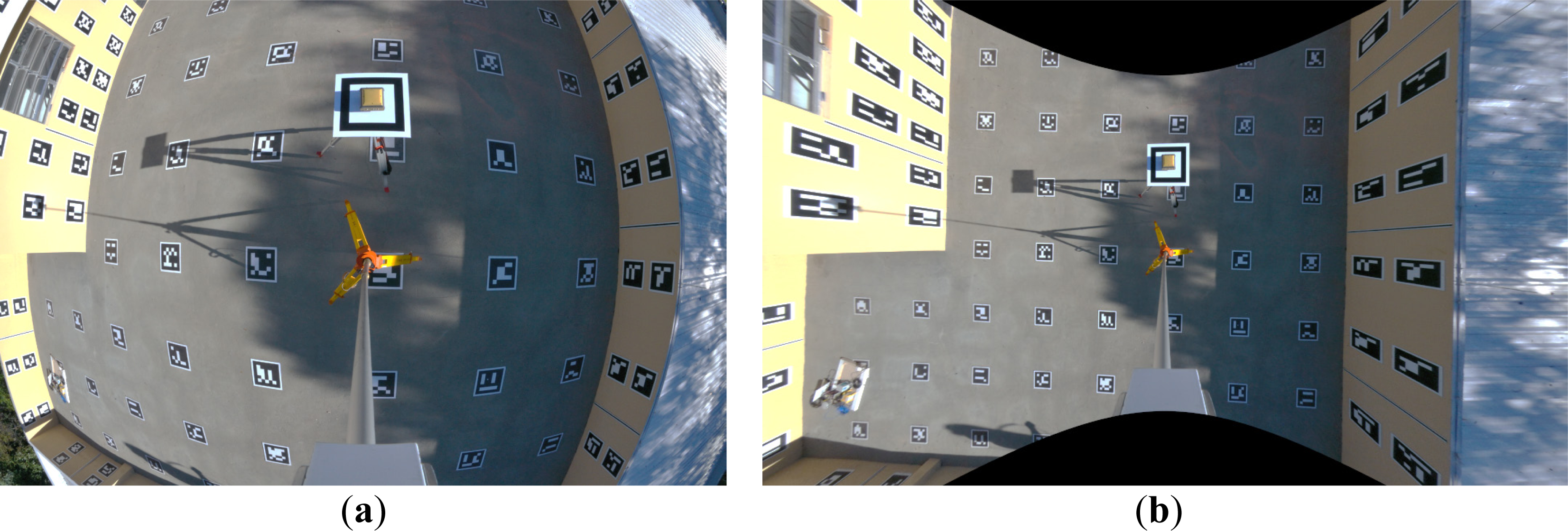
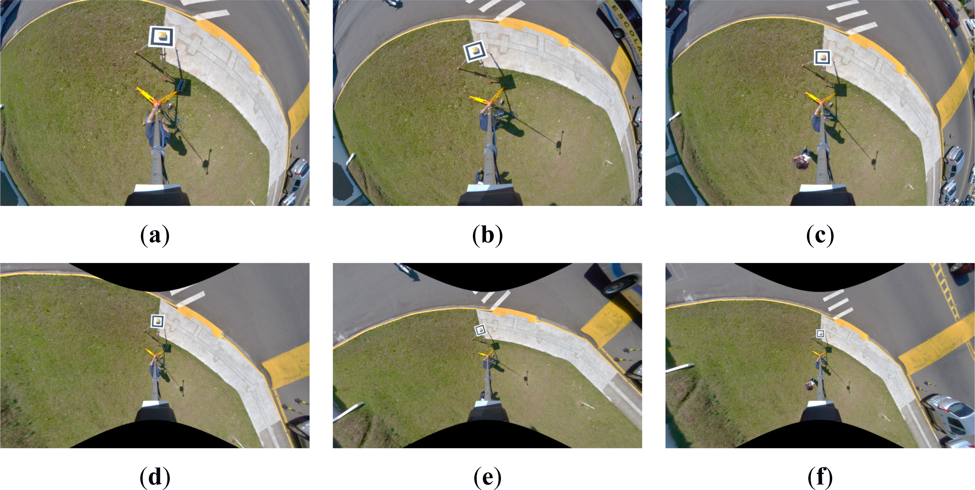
2.3. Automatic Target Detection

The corners of the square target over the panel should be automatically located to guarantee an automatic processing chain and high precision with respect to the image coordinates. These features will be used as the GCPs to determine the EOPs of the panoramic images using an indirect image orientation process.

If outdoor images are acquired, shadows may be present that affect their radiometric properties and hinder the automatic target detection and location (see Figure 3a). To overcome this problem, an algorithm developed by Freitas and Tommaselli [17] was used to perform shadow labeling and enhancement such that the shadow areas would have local histograms similar to those of the other areas, as shown in Figure 3b. The target detection process can be significantly improved using this local enhancement step.

The square target can be located using template matching, and its corners can be detected with existing interest operators (e.g., Harris and Stephens [18], Moravec [19] or Förstner [20]). Various algorithms can be found in the computer vision and photogrammetry literature. Schmid et al. [21] performed a comparative study that evaluated selected point detectors based on repeatability and information content. An overview on interest operators for close-range photogrammetry was published by Jazayeri and Fraser [22], who presented a summary in a development timeline that considered important algorithms since 1977, when Moravec introduced the concept of interest points.

Another possibility for locating the corners of the square target, which was applied in this work, uses the ARUCO targets developed by Garrido-Jurado et al. [23] with free software based on the Open Source Computer Vision Library (OpenCV). These targets have two main components: an external crown, which is a rectangle, and 5 × 5 internal squares able to code 10 bits of information. An adaptation was carried out to perform the location, identification and accurate measurement processes of the corners of the crown (reference square; see Figure 3). In the algorithm, concave contours with four corners are obtained and retained to extract the rectangles, and thus, the square target can also be automatically identified to obtain the eight corners (external and internal edges) with sub-pixel precision. The automatic target measurement was implemented and it was preferable because it is more accurate than the interactive measurement, since the control panel will always appear in the scenes.

The eight control points are defined with reference to the panel center, which was tracked via GNSS. The distances from the antenna centroid to the square corners were measured with a precision calliper rule, and the plane coordinates of the eight corners were estimated from these distances. Using these eight points as GCPs, the EOPs of the images can be computed via bundle adjustment using Equation (2) of the equidistant fisheye model. Tie points can be measured to improve the quality of bundle adjustment.

2.4. Generation of Multi-Scale Models

As depicted in Figure 4, the 3D position (X, Y, Z) of a point P can be reconstructed from its projected rays from multiple images, provided that the position and orientation of the camera are known.

Initially, a multi-scale model must be generated and oriented. The relative positioning of the telescopic pole with the GNSS tripod is directly measured in the field to obtain an initial approximation of the camera position that can be used as an approximated value or even as an observation in the bundle adjustment.

Because the coordinates of the square target are known, the eight corners are used to simultaneously estimate the EOPs via bundle adjustment for the images collected at different heights using the ground coordinates, independently whether the model is composed for original fisheye images or resampled images. To achieve this goal, the image coordinates of the control and tie points must be measured and their systematic errors corrected.

Bundle adjustment uses the least-squares method to solve a system of non-linear equations in which the image coordinates are the observations and the EOPs and the ground coordinates of the tie points are the unknowns.

Although only a narrow bundle is used, the resulting orientation is valid for the central area of the images. As a result, points close to the reference panel can be reconstructed with precision, and a point cloud can be produced.

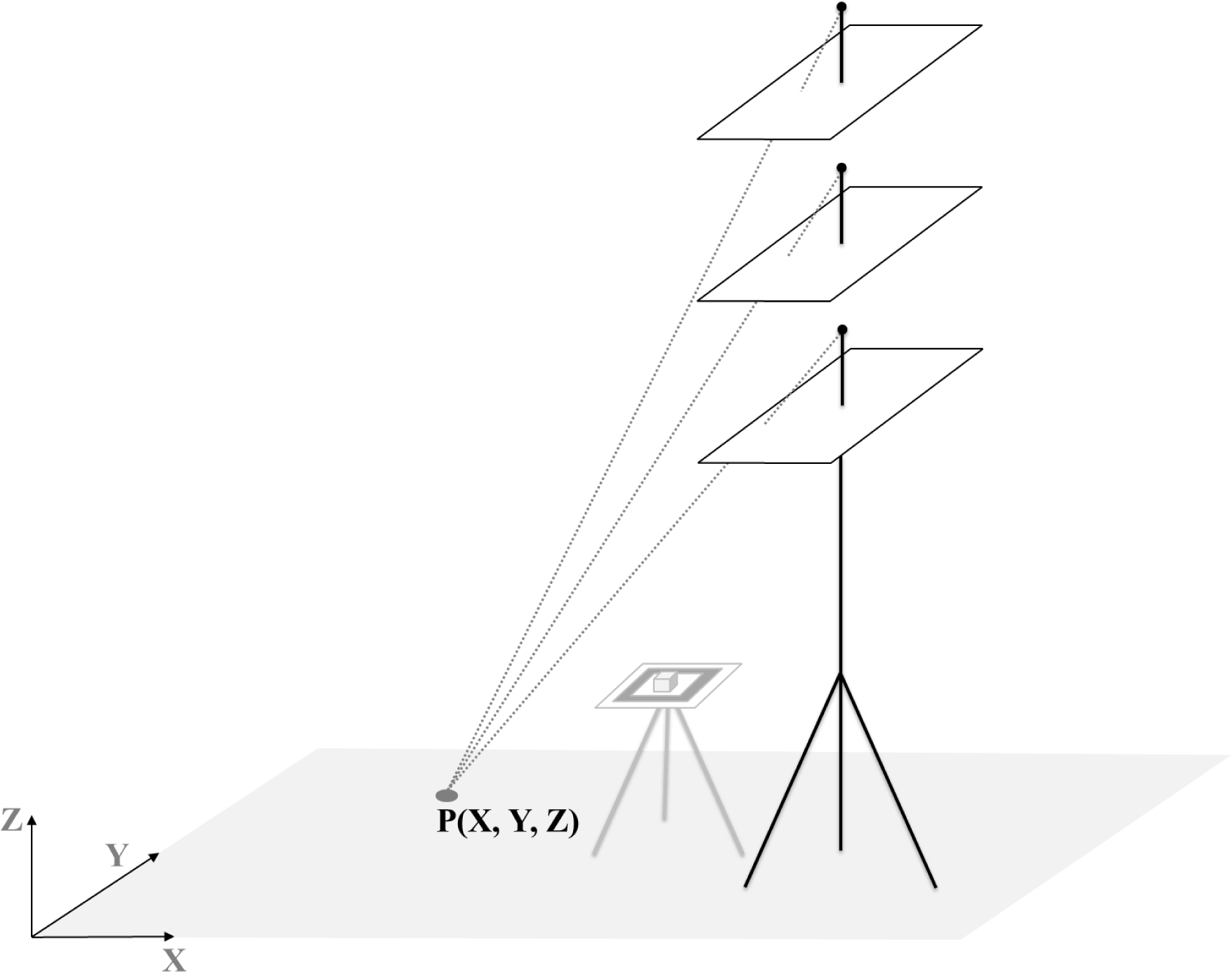
2.5. Determination of 3D Points

Once the images are oriented, the coordinates of the GCPs can be projected to the images using the collinearity equations to generate georeferenced templates that can be used in the orientation of aerial images [10]. However, if the inverse process is performed, image points are projected into the object space, and the 3D coordinates of ground points are determined by photogrammetric forward intersection.

An automatic process used to find corresponding points in multi-scale images of a scene can be developed using feature-based matching, e.g., with scale-invariant feature transform (SIFT) descriptors. The distinct features of an image are extracted based on the magnitude and orientation information from local gradients. The SIFT technique selects distinguishable points that enable multi scale matching for images with small differences in rotations. Furthermore, SIFT is flexible to changes in the camera viewpoint (further details on SIFT are provided in Lowe [24]). Lingua et al. [25] published a study on the performance of the SIFT technique, in which the operator was evaluated in photogrammetric tasks and the good performance of the SIFT operator was highlighted for feature extraction and image matching.

Application of SIFT enables the extraction of the most distinct points over a scene. In this paper, the descriptor points are matched and used as tie points in the bundle adjustment process, thus improving both the determination of the image EOPs and generating the 3D coordinates of points around the control panel.

With a point cloud, it is possible to generate a small DSM, DTM, and ortho-image, and the georeferenced templates are generated from this ortho-image for use as control scenes [10].

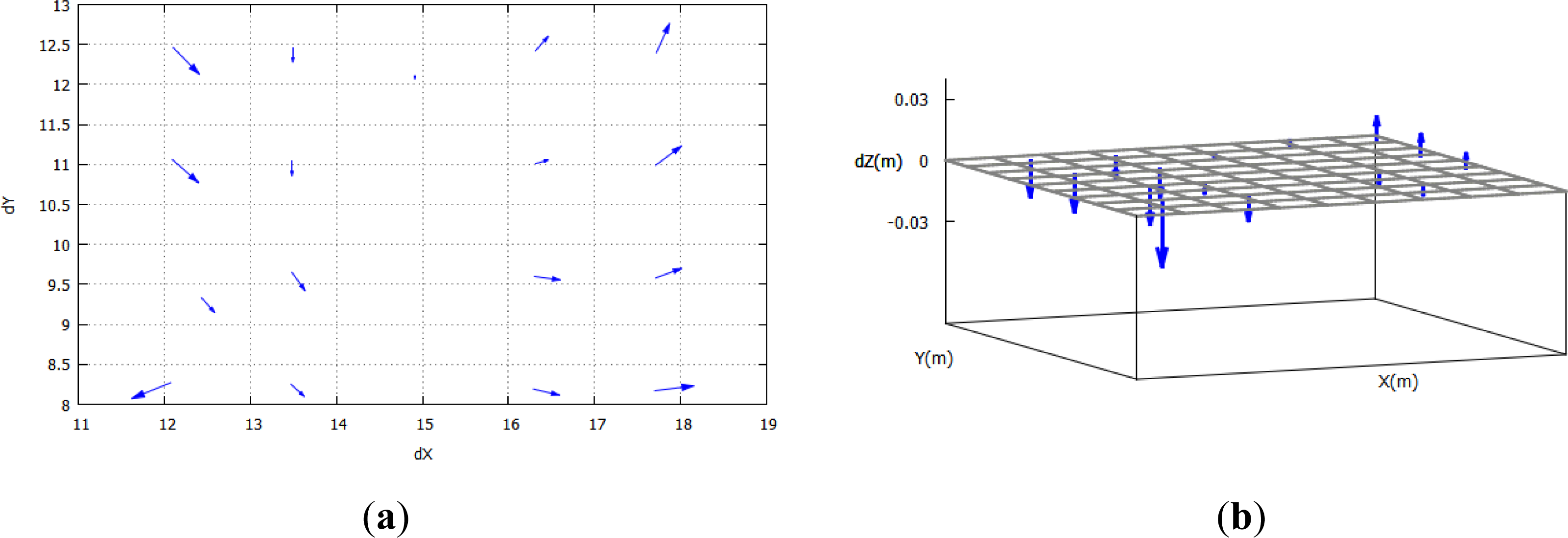
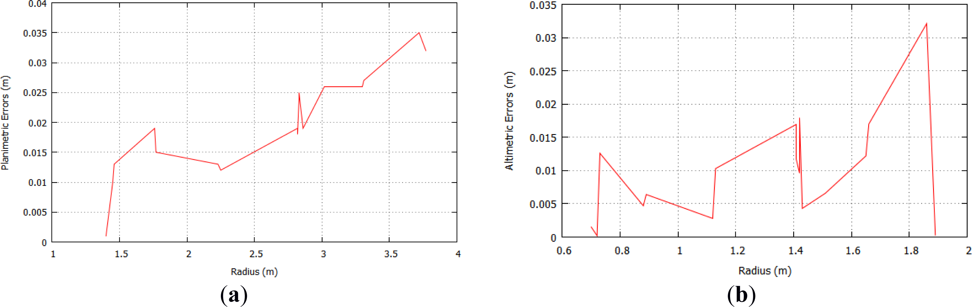
3. Experimental Results and Analysis

Section 3 presents experiments carried out to prove the concepts and to demonstrate the capabilities of the proposed approach.

Trials were developed in two scenarios:

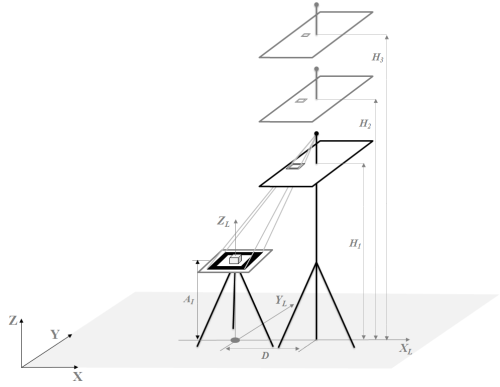
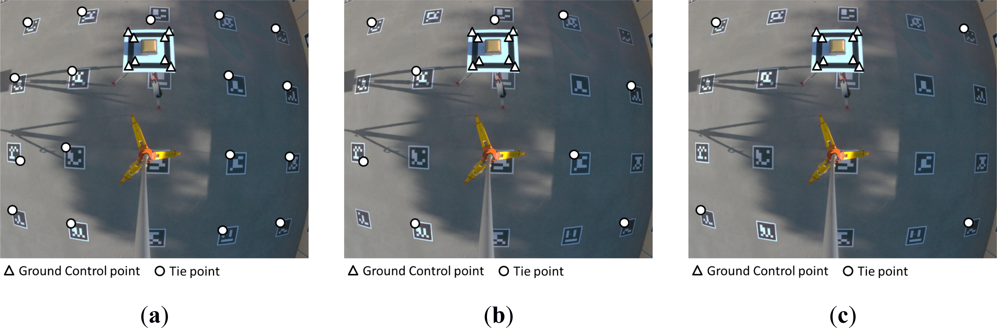
• The first trial was performed in a terrestrial calibration field mounted with ARUCO-coded targets with known terrestrial coordinates for automatic recognition. This test provided an assessment of the accuracy that can be achieved with the proposed technique based on the accurate coordinates of the targets in the calibration field.
• The second trial was applied in a typical area with distinct features to exemplify a practical application of the technique.

A Nikon digital camera with fisheye lenses (see

Table 1. Technical specifications for the image acquisition system.

Camera model	Nikon D3100
Sensor size	CMOS APS-C (23.1 × 15.4 mm)
Image dimension	4608 × 3072 pixels (14.2 megapixels)
Pixel size	0.005 mm
Nominal focal length	8.0 mm (Bower SLY 358N)

for technical details) was used to acquire the images for the experiments. First, the camera was calibrated in the same terrestrial test field using a bundle adjustment with the equidistant camera model and an additional Conrady-Brown lens distortion model, as presented in the next section.

3.1. Camera Calibration in the Terrestrial Test Field

The terrestrial calibration field is composed of 139 coded targets with ARUCO style regularly distributed on the floor and walls, as shown in Figures 1 and 3. A set of 16 images was acquired for the calibration process as follows. Twelve horizontal images were collected at three camera stations. At each station, four convergent images were acquired with changes in positions and rotations. In addition, four vertical images were also collected in the same position but at different heights. This procedure was used to minimize the linear dependency between the interior and exterior orientation parameters.

The corners of the ARUCO targets were automatically located over the 16 images, generating 6820 observations from 383 control points. The object coordinates of the corners were previously measured using topographic and photogrammetric methods with an accuracy of 3 mm.

In-house-developed software, implemented in C/C++ language and referred to as calibration with multi-camera (CMC), was modified to add the equidistant model [16] for the fisheye lens [26]. Then, the IOPs and EOPs were determined for the camera-lens system with bundle adjustment.

Table 2. interior orientation parameters (IOPs) estimated in the calibration process via bundle adjustment with the equidistant model.

Parameters	Estimated Values	Estimated Standard Deviations
f (mm)	8.3794	0.0011 (±0.23 pixels)
x0 (mm)	0.0729	0.0011 (±0.22 pixels)
y0 (mm)	0.0019	0.0009 (±0.18 pixels)
K1 (mm−2)	4.20 × 10−4	3.77 × 10−6
K2 (mm−4)	8.20 × 10−7	6.32 × 10−8
K3 (mm−6)	−2.54 × 10−9	3.12 × 10−1°
P1 (mm−1)	4.84 × 10−6	1.63 × 10−6
P2 (mm−1)	−2.28 × 10−7	1.67 × 10−6
A	3.34 × 10−5	1.88 × 10−5
B	−7.43 × 10−4	3.58 × 10−5
σ naught	0.0054 (≈1 pixel)

presents the IOPs estimated using the camera calibration process. These values were also used to produce the resampled images (Figure 5b).

To compare the results, both the original and resampled images were used to generate multi-scale models and estimate 3D point coordinates with bundle adjustment. The entire process for the determination of 3D points using the control panel was performed in the calibration field, and the results were analyzed based on discrepancies in the checkpoint coordinates to assess their accuracy.

3.2. Experiments in the Calibration Field

Following the procedure described in Section 2.2, three vertical images were acquired at different heights of 3.0, 3.5, and 4.5 m above the ground and at the same XY position. The acquired images presented values of ground sample distances (GSDs) ranging from 2 mm to 3 mm. The images formed a multi-scale model to be used in the accuracy assessment of the proposed technique.

The equidistant model for the fisheye lenses with the IOP values estimated by the calibration process was used to resample the vertical images and to correct the fisheye distortion, thus generating a conventional perspective view. Figure 5 provides an example of an original vertical image collected in the calibration field and its result after resampling.

In the bundle adjustment, image-processing software [23] automatically recognized the coded targets and their corners with sub-pixel precision.

Image orientation with bundle adjustment requires at least three control points with good distribution, normally located in the corners of the block of images. In the case of this technique, eight control points are provided by the reference panel but generate a narrow bundle of rays. This type of configuration is not suitable because the control points are concentrated in a small region near the image center. It is expected that points far from this ground point will produce higher errors. Nevertheless, it is relevant to experimentally assess the extent of these errors to verify whether these points are suitable for generating a small DTM around the surveyed GCP for ortho-generation.

Considering that the image orientation was computed from the ground control provided by the reference square, the accuracy of the estimated ground points is expected to decrease at locations far from this region. Therefore, the goal is to assess the accuracy in the area and to find a range that ensures the determination of 3D points with acceptable precision.

The CMC software was used to process the image bundle adjustment of the multi-scale models with respect to the local system of the terrestrial calibration field.

The object coordinates over the panel are known with high accuracy and were set with a standard deviation of σ = 0.0005 m. In the image space, all of the points were automatically located, and a standard deviation of σ = 0.5 pixels was considered.

The initial values of the EOPs (X_C, Y_C, Z_C, ω, φ, κ) can be introduced into the bundle adjustment considering two cases:

• Indirect determination: The known values of the EOPs are used as approximated values in the bundle adjustment. These values are obtained from the relative positioning between the GNSS receiver and telescopic pole with the estimated heights from the graduated rule in the telescopic pole. Standard deviations of σ = 0.5 m for the (X_C, Y_C, Z_C) position and σ = 30° for the attitude were configured in the bundle adjustment, meaning that this initial value will not have any influence on the solution.
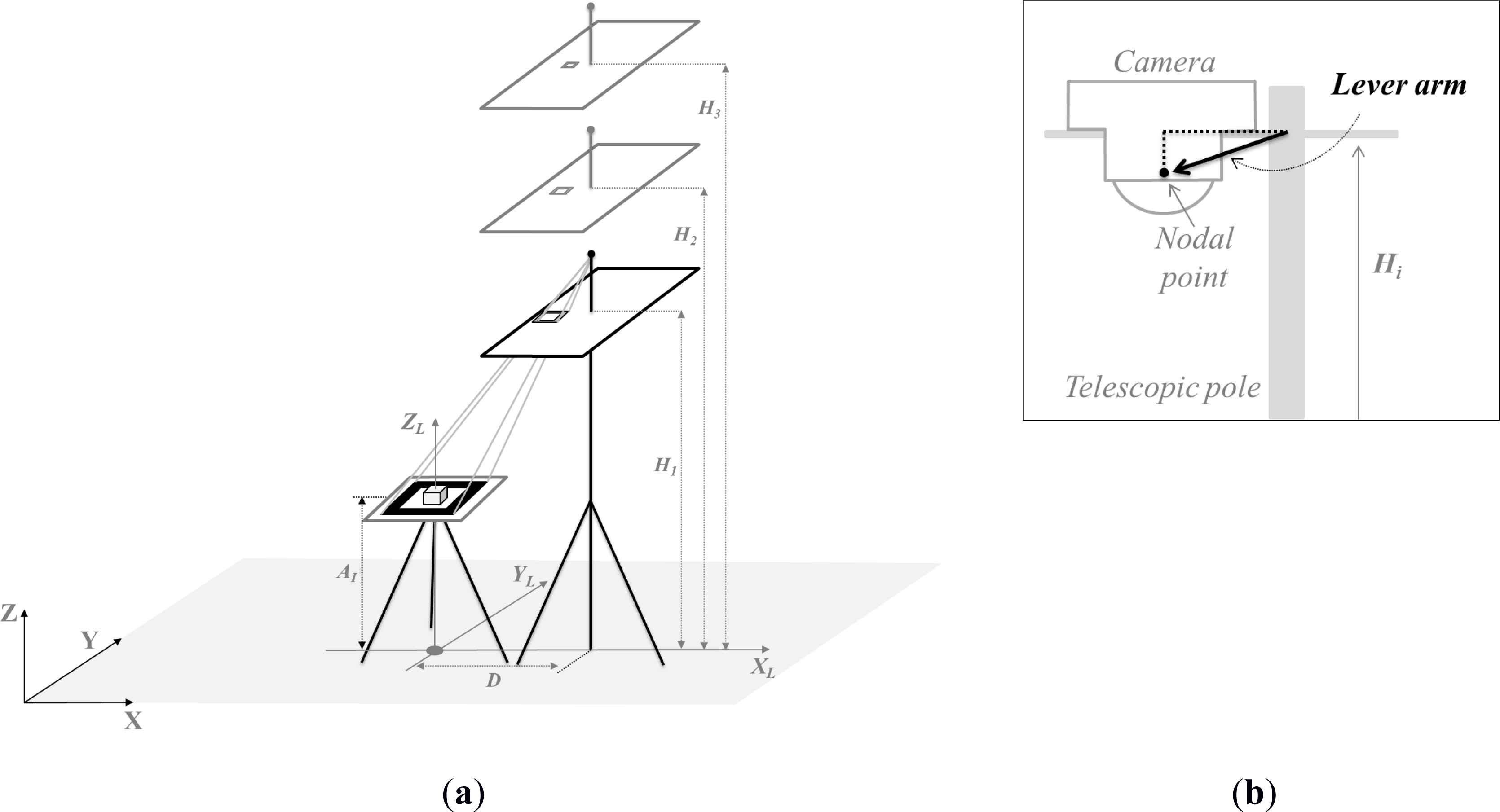
• Direct determination: The known values of the EOPs will be used as observations or weighted constraints in the bundle adjustment. These values are estimated using the distance directly measured between the GNSS receiver and telescopic pole, the heights were measured with an EDM, and the lever arm (displacement between the external lens nodal point and the platform supported by the pole; see Figure 2b) was previously estimated. The standard deviations of the camera positions were considered as σ = 10 cm in X_C and Y_C and σ = 5 mm in Z_C due to the displacements and movements involved in lifting the camera. For the attitude, the standard deviation was considered to be σ = 10°. These values likely will not have a significant role in the bundle solution.

The values of the standard deviations of the imposed constraints were defined based on tests performed in the calibration field to precisely check the actual range of variations in the coordinates of the platform. The sets of experiments were produced to verify the quality of the image bundle triangulation and the effects of introducing direct measurements of the camera positions into the 3D point determination.

First, the trials considered four vertical images, but trials were also performed with three images to consider a more practical procedure. The differences in the values of the estimated EOPs were less than 0.0001 m in (X_C, Y_C, Z_C), and therefore, the experiments were focused on the use of only three images. Use of a minimum number of images is important for accelerating the technical implementation without affecting the quality of the results.

The experimental assessment was performed based on discrepancies obtained from independent checkpoints, which were topographically measured in the field and were not included in the bundle adjustment.

Figure 6 presents one of the images used for the experimental assessment. Three multi-scale images were acquired over a flat surface with an area of approximately 20.25 m². One corner of each ARUCO target in the calibration test field was automatically identified with its 3D coordinate estimated by bundle adjustment and compared with the ground coordinates, whereas the eight GCPs in the square reference target can be observed in the upper region of the images. Only fully visible targets were recognized, making it possible to use their corners.

These eight corners in the reference target have known ground coordinates and were used to simultaneously estimate the EOPs of the three images. Several image points with known object coordinates were selected as tie points and were also included in the bundle adjustment to generate the 3D coordinates. Therefore, a comparison between the estimated coordinates of the tie points and their true values (check points) can be performed to assess the accuracy of these reconstructed points in the object space.

The number and distribution of tie points can contribute to the improvement of the bundle solution when using this proposed technique with ground control from a reference square. To assess the role of the tie points, three groups of image points were considered with changes in the point arrangement that covered the entire area, primarily in the most critical positions (far points). Next, three groups were organized for assessment as follows:

• Group I: Seventeen tie points within the scene to fully cover the area (Figure 6a);
• Group II: Nine distributed tie points (half of the total; Figure 6b);
• Group III: Four tie points at the corners of the model (Figure 6c).

The generation of 3D points was processed for both original and resampled images for comparison purposes, and the results are presented in the following paragraphs in this section.

Table 3. Root mean square errors (RMSEs) obtained with three different distributions of tie points using the original fisheye images.

Initial Values for the EOPs	Group I (17 Tie Points) RMSE (m)			Group II (9 Tie Points) RMSE (m)			Group III (4 Tie Points) RMSE (m)
	X	Y	Z	X	Y	Z	X	Y	Z
Indirect Determination	0.019	0.016	0.023	0.019	0.018	0.021	0.034	0.027	0.029
Direct Determination	0.013	0.017	0.013	0.013	0.019	0.010	0.026	0.032	0.011

refers to the bundle adjustment performed with the observations from the original images (with fisheye effects). The presented values are the root mean square errors (RMSEs) obtained from the differences between the estimated coordinates and independent surveyed coordinates (check points) in the object space. The results are organized according to the groups of tie points and the technique used to determine the initial EOP values.

The results achieved with both Groups I and II (without constraints in the EOPs; Table 3, second row) were similar, indicating that nine tie points are sufficient to achieve an accuracy of approximately 2 cm for the reconstructed points. However, the achieved accuracy was approximately 3 cm for the three coordinates in the borders of the model when only four tie points were used (Table 3, second row, Group III). The arrangement of Group III is important for demonstrating the magnitude of errors in the worst case, if only a minimum number of points is used in the area limits. In that case, the error was less than 3.5 cm, which is sufficient for the intended applications.

Although indirect determination with bundle adjustment enables ground discrepancies with an RMSE of approximately 3 cm, in general, imposing certain constraints in the EOPs from directly measured values provided smaller RMSEs in all groups (see Table 3, third row). The XY coordinates of the tie points were estimated with RMSEs of less than 2 cm, and the Z coordinate had RMSEs of less than 1.3 cm. The improvement in the accuracy of the tie points was nearly twofold for the Z coordinate, mainly because the constraints in Z_C could be imposed with higher weights than the constraints in X_CY_C due to the physical movements of the platform over the pole in X_CY_C.

A similar analysis is presented in

Table 4. RMSEs obtained for three quantities of tie points considering the resampled images.

Initial Values for the EOPs	Group I (17 Tie Points) RMSE (m)			Group II (9 Tie Points) RMSE (m)			Group III (4 Tie Points) RMSE (m)
	X	Y	Z	X	Y	Z	X	Y	Z
Indirect Determination	0.020	0.016	0.031	0.022	0.020	0.026	0.035	0.020	0.035
Direct Determination	0.011	0.017	0.023	0.011	0.020	0.018	0.019	0.025	0.026

but using the resampled images. In this case, the bundle adjustment was performed with the conventional collinearity equations.

Table 4 refers to the RMSEs obtained from the tie points considering the multi-scale model with the resampled images. The results for Groups I and II exhibited RMSEs of less than 0.031 m for the indirect determination and less than 0.023 m for the direct determination. These values were smaller than those of Group III. Again, as in Table 3, the direct determination provided more accurate results. Even if using only four points, the results were less than 0.026 m. A comparison of the results achieved from the resampled images (Table 4) with those obtained from the original distorted images (Table 3) illustrates that using the original images leads to better results. This result can be explained by the errors in the image measurement over the resampled images that are more blurred due to scale change and resampling.

Figure 7a depicts a needle map for the discrepancies in the XY coordinates in the object space considering the original images with 17 tie points in the area. It is possible to observe a systematic effect, which was expected due to the weak geometry provided by the control panel. As expected, the narrow bundle of rays on the GCP of the reference square is able to orientate the model in the central region of the images with high accuracy and generates more accurate ground points in the central area; however, this accuracy decreases as far as the point is with respect to the control square.

Figure 7b displays a graph for the discrepancies obtained in the Z coordinate. An inclination effect on the adjusted coordinates is observed, indicating more accurate values at the centre and larger discrepancies for more distant points. The differences ranged from −0.032 to 0.012 m with a standard deviation of ±0.008 m. The σ naught for all of the produced experiments had the same value of 0.01. This accuracy, even for the worst case, is sufficient to generate a small DTM and to create ortho-images for use as control scenes.

A further graphical analysis was performed for both the XY and Z coordinates. Figure 8a presents a graph generated by the planimetric errors (PEs) as a function of the radial distance from the panel center. The PEs were less than 2 cm at a radial distance of 1.4 m and increased up to 3.5 cm for a radial distance of 2 m.

Figure 8b presents the altimetric errors (AEs) calculated for the Z coordinate. The same AEs were less than 2 cm for a radius of 1.7 m; however, only one point caused the peak shown in the graph, and the remaining points were still within a range of errors from 0.0002 to 0.0018 m.

Based on the experiments performed in the calibration field with known ground coordinates, the results demonstrated that 3D coordinates could be generated with RMSEs less than 2 cm, considering both original and resampled images.

Some trials using nominal camera parameters (without camera calibration) were also performed with the bundle adjustment to assess the need for rigorous camera calibration. Discrepancies around 0.133 m in planimetry and 0.285 m in height were achieved mainly due to the non-corrected radial distortion effects and differences in the focal length. These results showed that the camera calibration is a fundamental step to achieve the intended results.

The experimental area was assessed in terms of the critical positions and with different tie point arrangements. As a result, it is possible to ensure that areas of approximately 16 m² (approximately 21 × 21 pixels) can be used to derive such products as small models, ortho-images, or georeferenced terrestrial chips for matching with aerial images (in this case, up to 20 cm of GSD).

3.3. Experiments in Areas with Distinct Features

A further experiment considering distinguishable features in an area was also conducted to illustrate how the approach could be used in a practical application of the proposed application for scene reconstruction. Only areas with certain distinct features were considered.

After selecting an area, the surveying and imagery devices were positioned. The reference square was north-oriented, and the distances between the devices were measured. Images were collected at three heights, and one GCP was surveyed.

In this case, the GNSS positioning was based on a point feature for later verification by manual/interactive inspection. However, the GNSS receiver could be installed in any other position covering the area, even in a homogeneous area.

For the bundle adjustment, standard deviations were set with the same values used in the experiments in the calibration field, and initial approximations to the EOPs were carried out based on the measures directly collected in the field.

Figure 9 presents two multi-scale models used for the trials. The first model is composed of the original images considering fisheye geometry effects, whereas the second model uses the resampled images.

Automatic tie points were generated using the SIFT technique, and homologue points were obtained by matching between descriptors. The object coordinates of these tie points were estimated via the bundle adjustment in both models, similar to the experiments in the calibration field.

Figure 10a displays points matched in an image triplet to automatically generate tie points. From the previously presented experiments, it is known that additional points provide better results. With this technique, the 3D coordinate of any point appearing in two or three images can be determined in the object space.

To generate an ortho-image without the control panel, as shown in Figure 10b, the last image was acquired in the highest position after removing the GNSS receiver and the reference target. The image coordinates of some tie points were inserted in the block to be adjusted with the previous images containing control targets. Tie points were determined by SIFT among all images and then the last image was oriented in the bundle adjustment. The estimated 3D coordinates of the tie points were used to generate a small DTM, which enabled to ortho-rectify the image.

The image of the telescopic pole can be removed using a previously defined mask. The choice of the pole position is important, since the operator previously knows the interest area and the region to be occluded before mounting the imagery system. The interest area will not be occluded and the area occluded by the pole can be either a homogenous or an area with unimportant features.

The generated coordinates were determined in a local system, and a transformation is required to transform these coordinates to, for instance, the UTM coordinate system. If a compass is used to measure the azimuth, this value can be used provided that corrections for magnetic declination and meridian convergence are introduced (see Blachut et al. [27]). Another technique involves the installation of a GNSS receiver over the camera and transformation of the resulting images to a geographic coordinate system with better accuracy compared with that of the compass measurement. The impact of this choice will depend on the intended application, and this assessment is left as a suggestion for future work.

4. Conclusions

This paper introduced an original technique for automatic determination of 3D point coordinates from close-range photogrammetric images with minor interactive interventions. The full pipeline was demonstrated, from the camera calibration process through to the generation of 3D points. An arrangement of terrestrial images with vertical displacements was also presented to generate a multi-scale model. The adopted configuration was intended to render field surveys more practical, without the need to change the tripod and camera, as in the conventional technique for acquisition of multiple images to form stereo pairs.

The proposed method can be used to generate cloud points that can serve not only as control points but also can be used to generate ortho-rectified control scenes (see Figure 10b). Using a square target attached to a GNSS receiver, areas with distinct features can be selected for recovery of their 3D coordinates. Some limitations and advantages of the presented technique can be mentioned.

Limitations:

• Occlusions can occur at the limits of these multi-scale images; however, the central area is not occluded because the receiver must be always positioned in open areas to collect GNSS signals.
• The geometry is not optimal, but it is sufficient to reconstruct the central region of the image. If a second camera station is added, the geometry can be improved but at the cost of some additional operations;
• Only small areas are reconstructed, but large enough to cover the main features of a scene.

Advantages or contributions:

• The image acquisition is performed while the GCP is being surveyed. There is no additional time delay to take these pictures. Only a few additional measurements are required (horizontal and vertical distance between the GNSS receiver and the camera). The time for images acquisition is compatible with the GNSS surveying period; also, the entire system can be mounted in a few minutes;
• There is no need to change the pole position as in a conventional stereo pair acquisition. The image acquisition does not add remarkable complexity into the surveying process;
• The operator can be the same surveyor that set the GNSS receiver. No expert operator is required as in the case of using an UAV;
• High-resolution terrestrial images of the GCPs (GSD less than 3 mm) can be obtained and consequently used to generate the ortho-images to serve as control chips populating an image database;
• The control panel can be positioned in any area covering distinct features. The technique does not depend on point features (which are not always available anywhere). Areas can also be used in the image matching procedures;
• The acquisition technique and multi-scale processing are original;
• There is no significant investment with materials.

Experiments were carried out in a calibration field for accuracy assessment. If only four points in the corners of the model were inserted as tie points in the bundle adjustment, the greatest RMSE presented a value of 3.5 cm. This value was reduced to less than 2 cm when additional tie points were added to the calculation. The difference between using 17 points and nine points was shown to be negligible, indicating that nine tie points suffice.

Based on independent checkpoints, in the best case (Table 3), the approach achieved accurate values of approximately 1.7 cm for the reconstructed points within the assessed area of approximately 20 m². If less accurate data are required, slightly larger areas can be used. In any case, this approach is feasible to generate a 3D point cloud, which can produce a small DTM or DSM or an ortho-image for a flat or sloping area. Therefore, a georeferenced template can be extracted from the point cloud.

Using the resampled images also leads to acceptable results, but the accuracy was slightly higher using the original images. This observation is important because further steps are avoided, and the measurements can be performed directly using the original distorted images provided that corrections are later applied in the image coordinates before bundle adjustment. To further improve the automation of this technique, a connection between the camera and notebook via Bluetooth technology can be easily implemented, and the data flow can occur simultaneously with the GNSS tracking.

In conclusion, the results based on the analysis of checkpoints achieved discrepancies of less than 2 cm for the 3D point determination in a small area, which was the scope of study. In addition, the potential to automate the technique was also demonstrated, and future work should be carried out to evaluate the generated products, such as terrestrial templates for ground control for aerial or orbital images.

References

1. Dandois, J.P.; Ellis, E.C. Remote sensing of vegetation structure using computer vision. Remote Sens 2010, 2, 1157–1176. [Google Scholar]
2. Wondie, M.; Schneider, W.; Melesse, A.M.; Teketay, D. Spatial and temporal land cover changes in the Simen Moutains national park, a world heritage site in northwestern Ethiopia. Remote Sens 2011, 3, 752–766. [Google Scholar]
3. Nakano, K.; Chikatsu, H. Camera-variant calibration and sensor modeling for practical photogrammetry in archeological sites. Remote Sens 2011, 3, 554–569. [Google Scholar]
4. Harwin, S.; Lucieer, A. Assessing the accuracy of georeferenced point clouds produced via multi-view stereopsis from unmanned aerial vehicle (UAV) imagery. Remote Sens 2012, 4, 1573–1599. [Google Scholar]
5. Tommaselli, A.M.G.; Galo, M.; Moraes, M.V.A.; Marcato Junior, J.; Caldeira, C.R.T.; Lopes, R.F. Generating virtual images from oblique frames. Remote Sens 2013, 5, 1875–1893. [Google Scholar]
6. Gülch, E. Automatic Control Point Measurement. In Proceedings of the Photogrammetric Week’95, Heidelberg, Germany, 11–15 November 1995; pp. 185–196.
7. Heipke, C. Automation of interior, relative, and absolute orientation. ISPRS J. Photogramm. Remote Sens 1997, 52, 1–19. [Google Scholar]
8. Hahn, M. Automatic Control Point Measurement. In Proceedings of the Photogrammetric Week’97, Heidelberg, Germany, 22–26 September 1997; pp. 115–126.
9. Jaw, J.-J.; Wu, Y.-S. Control pacthes for automatic single photo orientation. Photogramm. Eng. Remote Sens 2006, 72, 151–157. [Google Scholar]
10. Berveglieri, A.; Marcato Junior, J.; Moraes, M.V.A; Tommaselli, A.M.G. Automatic Location and Measurement of Ground Control Points Based on Vertical Terrestrial Images. In Proceedings of Remote Sensing and Photogrammetry Society Conference, London, UK, 12–14 September 2012.
11. Remondino, F.; El-Hakim, S. Image-based 3D modeling: A review. Photogramm. Rec 2006, 21, 269–291. [Google Scholar]
12. Barazzetti, L.; Scaioni, M.; Remondino, F. Orientation and 3D modeling from markerless terrestrial images: Combining accuracy with automation. Photogramm. Rec 2010, 25, 356–381. [Google Scholar]
13. Luhmann, T; Robson, S.; Kyle, S.; Harley, I. Close Range Photogrammetry: Principles, Techniques and Applications; Whittles Publishing: Scotland, UK, 2006; p. 510. [Google Scholar]
14. Brown, D.C. Close-range calibration. Photogramm. Eng 1971, 37, 855–866. [Google Scholar]
15. Habib, A.F.; Morgan, M.F. Automatic calibration of low-cost digital cameras. Opt. Eng 2003, 42, 948–955. [Google Scholar]
16. Schneider, D.; Schwalbe, E.; Maas, H.G. Validation of geometric models for fisheye lenses. ISPRS J. Photogramm. Remote Sens 2009, 64, 259–266. [Google Scholar]
17. Freitas, V.L.S.; Tommaselli, A.M.G. An Adaptive Technique for Shadow Segmentation in High-Resolution Omnidirectional Images. In Proceedings of the IX Workshop de Visão Computacional, Rio de Janeiro, Brazil, 3–5 June 2013.
18. Harris, C.; Stephens, M. A. Combined Corner and Edge Detector. In Proceedings of the 4th Alvey Vision Conference, Manchester, UK, 31 August–2 September 1988; pp. 147–151.
19. Moravec, H.P. Towards Automatic Visual Obstacle Avoidance. In Proceedings of the 5th International Joint Conference on Artificial Intelligence, Cambrigde, MA, USA, 22 August 1977.
20. Förstner, W. A. Feature based correspondence algorithm for image matching. Int. Arch. Photogramm. Remote Sens. Spat. Inf. Sci 1986, 26, 150–166. [Google Scholar]
21. Schmid, C.; Mohr, R.; Bauckhage, C. Evaluation of interest point detectors. Int. J. Comput. Vis 2000, 37, 151–172. [Google Scholar]
22. Jazayeri, I.; Fraser, C. Interest operators for feature based matching in close range photogrammetry. Photogramm. Rec 2010, 25, 24–41. [Google Scholar]
23. Garrido-Jurado, S.; Muñoz-Salinas, R.; Madrid-Cuevas, F.J.; Marín-Jiménez, M.J. Automatic generation and detection of highly reliable fiducial markers under oclusion. Pattern Recognit 2014, 47, 2280–2292. [Google Scholar]
24. Lowe, D.G. Distinctive image features from scale-invariant keypoints. Int. J. Comput. Vis 2004, 60, 91–110. [Google Scholar]
25. Lingua, A.; Marenchino, D.; Nex, F. Performance analysis of the SIFT operator for automatic feature extraction and matching in photogrammetric applications. Sensors 2009, 9, 3745–3766. [Google Scholar]
26. Tommaselli, A.M.G.; Polidori, L.; Hasegawa, J.K.; Camargo, P.O.; Hirao, H.; Moraes, M.V.A.; Rissate Junior, E.A.; Henrique, G.R.; Abreu, P.A.G.; Berveglieri, A.; et al. Using Vertical Panoramic Images to Record a Historic Cemetery. In Proceedings of the XXIV International CIPA Symposium, Strasbourg, France, 2–6 September 2013.
27. Blachut, T.J.; Chrzanowski, A.; Saastamoinen, J.H. Map Projection Systems for Urban Areas. In Urban Surveying and Mapping; Springer-Verlag: New York, NY, USA, 1979; pp. 12–41. [Google Scholar]
Figure 1. (a) Devices used to acquire vertical images and GNSS coordinates; (b) Panel with the square target.
Remotesensing 06 03020f1
Figure 2. (a) Survey of a point using the GNSS receiver and image acquisition with variation in height. (b) Relationship between the pole axis and the camera external nodal point.
Remotesensing 06 03020f2
Figure 3. (a) Original image with shadow. (b) Image after the shadow labeling and enhancement.
Remotesensing 06 03020f3
Figure 4. Multi-scale model for the 3D determination of point P.
Remotesensing 06 03020f4
Figure 5. Example of a vertical image acquired in the calibration field: (a) original fisheye image and (b) resampled image.
Remotesensing 06 03020f5
Figure 6. Assessment area with eight control points and varying number of tie points: (a) 17, (b) nine, and (c) four.
Remotesensing 06 03020f6
Figure 7. Needle map for (a) XY and (b) Z coordinates produced from the discrepancies between the estimated coordinates and their 17 tie points.
Remotesensing 06 03020f7
Figure 8. Graph comparing the errors against the radial distance from the panel center: (a) PE in the XY coordinates and (b) AE in the Z coordinate.
Remotesensing 06 03020f8
Figure 9. Multi-scale models with original images from (ac) and resampled images from (df).
Remotesensing 06 03020f9
Figure 10. (a) SIFT matching among images to automatically generate tie points. (b) ortho-image generated for the central area without the control panel.
Remotesensing 06 03020f10