The Use of Airborne and Mobile Laser Scanning for Modeling Railway Environments in 3D

Abstract

This paper presents methods for 3D modeling of railway environments from airborne laser scanning (ALS) and mobile laser scanning (MLS). Conventionally, aerial data such as ALS and aerial images were utilized for 3D model reconstruction. However, 3D model reconstruction only from aerial-view datasets can not meet the requirement of advanced visualization (e.g., walk-through visualization). In this paper, objects in a railway environment such as the ground, railroads, buildings, high voltage powerlines, pylons and so on were reconstructed and visualized in real-life experiments in Kokemaki, Finland. Because of the complex terrain and scenes in railway environments, 3D modeling is challenging, especially for high resolution walk-through visualizations. However, MLS has flexible platforms and provides the possibility of acquiring data in a complex environment in high detail by combining with ALS data to produce complete 3D scene modeling. A procedure from point cloud classification to 3D reconstruction and 3D visualization is introduced, and new solutions are proposed for object extraction, 3D reconstruction, model simplification and final model 3D visualization. Image processing technology is used for the classification, 3D randomized Hough transformations (RHT) are used for the planar detection, and a quadtree approach is used for the ground model simplification. The results are visually analyzed by a comparison with an orthophoto at a 20 cm ground resolution.

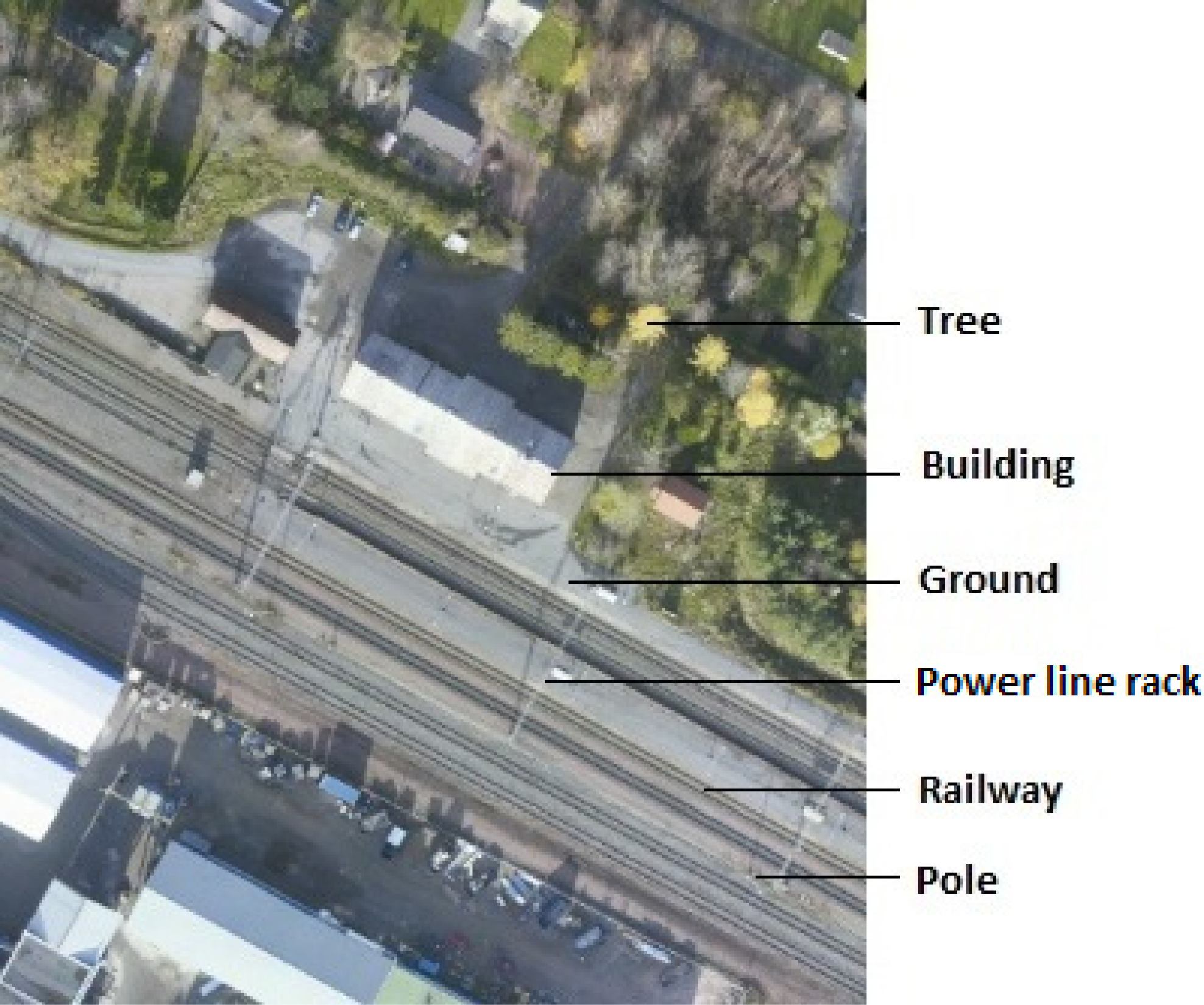
1. Introduction

Over the last five years, an estimated US $300 billion worth of global investment has been expended to maintain and upgrade railway networks. The top industry challenges are capacity, operational efficiency and reliability, structural and competition issues, and safety and security. Railway environments have a great influence on greenhouse gas emissions [1], because 80% of rail traffic in Europe is currently powered by electricity; therefore, the vast majority of trains emit no local air pollutants, and increased rail traffic can help achieve substantial progress towards the 2020 target of a 20% cut in the EU greenhouse gas emissions. MarketLine [2] predicted that the industry will grow by 24% (almost $210 billion) in the five-year period ending in 2015. The need to maintain better documentation of the existing railway environment has been stressed, and a quicker and more efficient method for inspecting railways is required. The increased growth of the EU railway industry has also impacted the use of laser scanning and photogrammetric techniques for railroad engineering.

The development of the railway industry has resulted in an increased demand for 3D modeling of railway environments because it provides an opportunity to visualize, explore and plan railway scenes indoors. However, because of the complexity of the terrain in railway environments, the available data sources for recent 3D modeling of such scenes have been mainly from aerial views, including aerial images, airborne laser scanning (ALS), orthophotos, digital elevation models (DEMs), and ground plans. The modeling from those data sources usually produces rough results (see Figure 1). It is challenging work to produce high resolution ground-based 3D modeling. The challenges result from the following: (i) complex terrains make it difficult to acquire data, especially for ground-based data collection; (ii) complex environments make it difficult to reconstruct environments. However, currently available sensor technologies and modeling methodologies have presented opportunities for detailed modeling of railway environments.

The rapid development of mobile sensor technology has made it possible to acquire data from complex terrains and scenes because of its flexible platforms, such as aircraft, cars or van, trains, boats, trolleys or personal backpacks. A laser scanner based on a platform of an aircraft is called an ALS and has been applied for surveying since 1994. After decades of development, the accuracy and density of point collection has been greatly improved. For instance, in 1993, the pulse repetition frequency (PRF) of ALS was 2 kHz, whereas in 2007, the best PRF of ALS was 200 kHz and in 2013, it had increased to 800 kHz. The point density has increased from a few points per m² to the current usual density of 50 points per m². Thus far, ALS has been a particularly important method of rapid and highly accurate large-area mapping, especially for DEM products. However, ALS offers data from the top view, which is not adequate for high resolution and ground-based object modeling. Ground-based mobile laser scanning (MLS) might provide complementary measurements for ALS. MLS is integrated with GNSS and inertial measurement unit (IMU) and contains single or multiple laser scanners mounted on a platform on a car, van or train. MLS can apply different point densities, scanning angles and ranges to the objects compared to ALS. State-of-the-art MLS has a scan rate of 400 lines per second; the MLS RIEGL VMX-450-RAIL (RIEGL, USA) can measure up to 1.1 million points per second along the trajectory of a moving platform with a 360° field of view without gaps [3]. The measurement distance to the objects can be from 0.3 m to 800 m. MLS can also be used with different platforms, such as vehicle- and trolley-operated MLS for urban area data acquisition, boat-mounted MLS equipment for fluvial environments, and backpack versions of MLS used for surveying applications in the field of natural sciences, an example of which can be found in Kukko et al. [4].

When reconstructing a complex railway environment, the complexity is based on the diversity of the objects of the railroad infrastructure and surroundings, which include railroads, buildings, powerlines, pylons, street/traffic lights, etc. Due to flexible sensor platforms offering various data sources, e.g., ALS and MLS, and also various available survey products like digital maps or ortho-photos, these data have provided the possibility for the complex 3D environment reconstruction. The multiple complementary data sources from different views offer the flexibility and feasibility required for rapid, highly efficient and detailed 3D environment modeling. The contributions of published studies on 3D modeling are listed below.

(i)

Building extraction and reconstruction

The methods for 3D building modeling rely heavily on data sources. Data from the field of photogrammetry, such as single images, stereo-images or multiple images, extract edge features or line-shaped objects, which provides significant benefits. However, planar feature extraction usually relies on texture recognition, which has considerable impacts on an object’s reflection, the light source, the angle of illumination, the position of the camera, etc. Therefore, it is more reliable to acquire planar features from laser scanning point clouds. However, the edge feature in point cloud scanning exhibits a saw-tooth shape and additional work is required to generalize the feature for the final line-shape acquisition. For building reconstruction, two techniques are usually applied: a model-driven approach and data-driven approach. Model-driven approaches construct the models by predefined primitives, whereas data-driven approaches utilize complex algorithms, such as plane detection, shape generalization, intersection line detection, to achieve the final model. A comparison between model-driven and data-driven methods has been conducted by Tarsha-Kurdi et al. [5]. According to their study, model-driven approaches rely on prior knowledge wherein people know a scene well and know what kind of building types are in a scene. Nevertheless, models based on this approach usually show less visual deformation compared to data-driven approaches. An advantage of data-driven approaches is that they do not require prior knowledge of a scene. Therefore, they can be applied to large unknown areas. Currently 3D models towards the whole world are going on [6]. It will require years until completion. Thus, automatic methods must still be developed and improved.

Literature reviews on the methods of building extraction and reconstruction can be found by Wang [7], Hyyppa et al. [8], Baltsavias [9], Brenner [10], Kaartinen and Hyyppa [11], and Haala and Kada [12]. Wang [7] produced an overview of the methods according to different data sources. Hyyppa et al. [8] produced an overall review for the methods of building extraction and reconstruction from single to multiple data sources since the 1990s. Kaartinen and Hyyppa [11] collected building extraction methods from 11 research agencies in 4 testing areas. Input data contained airborne-based data and ground plans (for selected buildings). Building extraction methods were analyzed and evaluated from the aspects of the time consumed, level of automation, level of detail, geometric accuracy, and total relative building area and shape dissimilarity. Haala and Kada [12] reviewed building reconstruction approaches according to building structures, such as roofs and facades, in which the input data covered both airborne-based and ground-based data.

In addition, Rutzinger [13] investigated the accuracy of data fusion of building walls and roofs from MLS and ALS, respectively, and verified their availabilities for 3D building modeling.

According to the previous research work, it can be concluded that the use of aerial-based data and ground-based data can achieve 3D building models with a (i) high level of automation and (ii) high level of detail.

(ii)

Powerline and pylon modeling

The available approaches to modeling powerlines can be obtained from Melzer and Briese [14], McLaughlin [15], Jwa et al. [16], and Sohn et al. [17]. Melzer and Briese (2004) proposed a method for powerline extraction and modeling via ALS by using a 2D Hough transformation and 3D fitting methods. However, it was based on the assumption that the powerlines were parallel. In practical applications, the scenes are usually more complex. Jwa (2009) introduced a voxel-based piece-wise line detector (VPLD) approach for automatic powerline reconstruction using ALS data. This method was based on certain assumptions such as the transmission line not being disconnected within one span and the direction of the powerline not changing abruptly within a span. The latest contribution to powerline classification and reconstruction using ALS data was by Sohn et al. (2012); they used a Markov random field (MRF) classifier to discern the spatial context of linear and planar features, such as in a graphical model for powerline and building classification. They assumed that powerlines run through inhabited areas with many buildings. Powerline pylons were classified and showed the connection between powerlines.

(iii)

Pole detection

Pole-like objects such as street lights or traffic lights are essential in railway environments. Studies about pole detection methods can be found in Brenner [18], Golovinskiy et al. [19], Lehtomäki et al. [20], Pu et al. [21], and Li and Elberink [22]. Golovinskiy et al. [19] utilized computer vision knowledge for object recognition (including poles) by the following four steps: locating, segmenting, characterizing, and classifying clusters of 3D points. The resulting recognition rate is 65%. Lehtomaki et al. [20] proposed an automatic method for pole-like object detection in MLS, and the algorithm is divided into four phases: (i) segment each profile into a group; (ii) remove the long group; (iii) cluster and merge the groups; and (iv) classify poles and non-poles according to their shape, length, orientation and point density in the local neighborhood of the cluster. The algorithm was evaluated and achieved a comparable accuracy, with a correctness of 81% and a detection possibility of 77.7%. Li and Elberink [22] proposed a five-step method of pole-like object detection. The accuracy of detecting pole-like objects was 72.4% and 75.1% in two different test datasets. However, most proposed methods were knowledge-based methods that required prior knowledge of the environment or scene.

(iv)

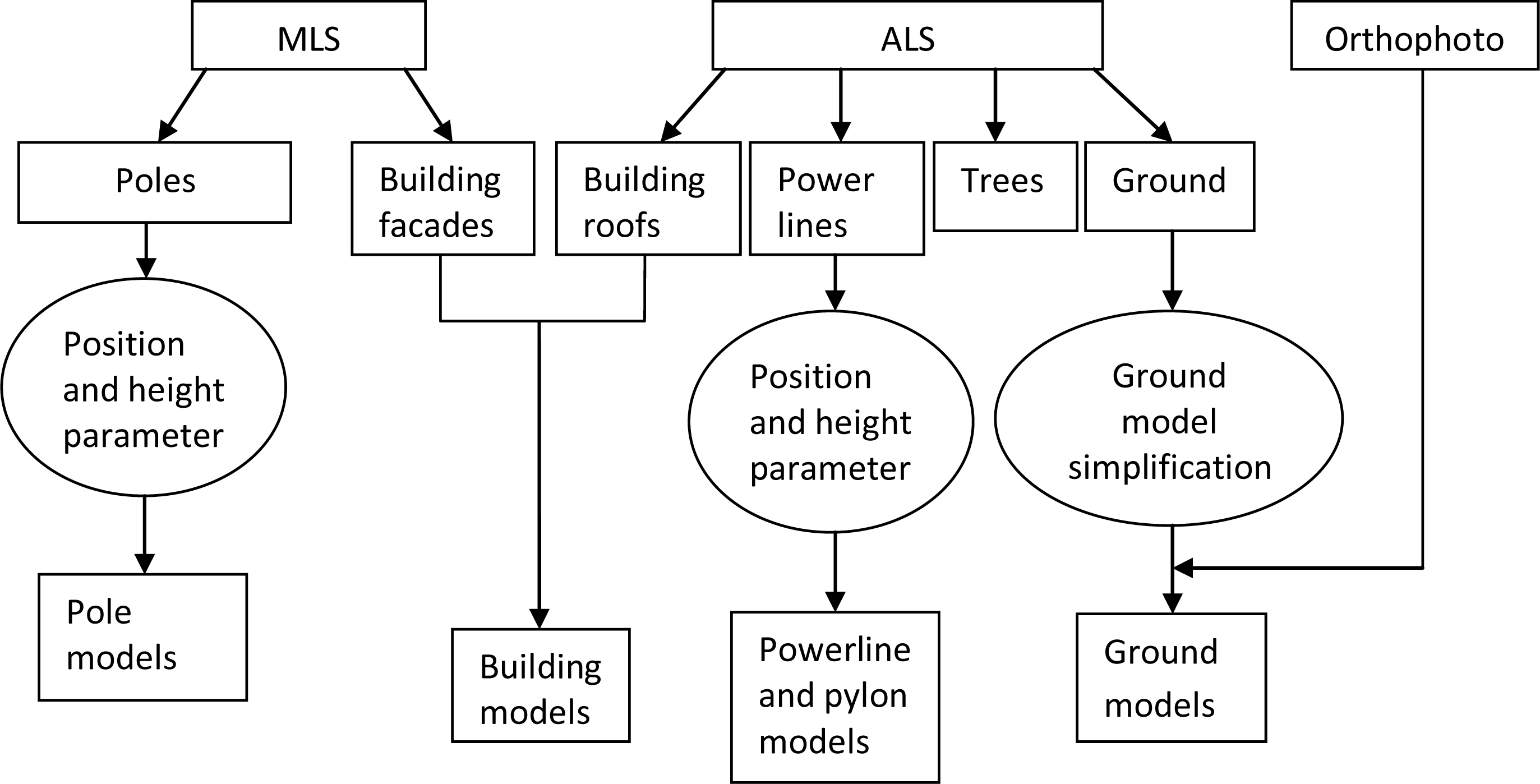
Road modeling

Studies of road extraction usually use images ([23–25]), ALS ([26–28]) or both ([29,30]) as data sources. Currently, certain methods based on MLS data are also available: Goulette et al. [31], Kukko [32], Jaakkola et al. [33] and Pu et al. [21]. MLS provides direct information to acquire the positions of railroads if the trajectory of the MLS fits the center line of one of the railroads. Searching for parallel lines could be helpful for other railway environment extractions. In this paper, the goal was to produce a final visualization of railway environments. Therefore, the visualization of railroads was conducted by mapping orthophotos onto ground models, with railroads considered part of the ground.

Additionally, currently 3D visualization has received considerable attention due to the large screen, the powerful processors and abundant memory as well as open operation system of the computer and the mobile devices, e.g., iPad, smartphone, or PDA [8]. However, as sensor technology continues to develop, it not only increases the number of point clouds but also the accuracy of data acquisition, although 3D models from a significant number of points would cause difficulties in the model post-processing, including model rendering and visualization, especially for dense ground points. Therefore, model simplification is required. Ground models are popularly called digital elevation models (DEMs), and they utilize raster format or vector format to represent terrain characteristics. Before the advent of ALS, the photogrammetric method was used as a primary method of DEM generation and included breakline extraction from stereo-images. DEM generation has primarily been in a vector format. ALS has become a very important method of DEM generation because of its rapid, accurate, and highly efficient data acquisition, especially over large survey areas. DEM is usually extracted from ALS as a raster. Raster DEMs present flat or undulated terrain as points with uniform spaces. Disadvantages include redundant points for flat terrain and inadequate representation in a changing or sloped area. Numerous methods for DEM simplification have been reported, and the main methods are as follows [34]: (i) working from a finer resolution of DEM to a coarse resolution for a point reduction method; (ii) reconstructing the terrain by a triangulated irregular network (TIN) method; (iii) filtering method; (iv) point-additive method; (v) point-subtractive method; (vi) feature-point method; and (vii) combination of the point-additive and feature-point methods [34]. This paper will present a novel and effective approach for ground point simplification that has adjustable parameters for the different levels of detail of the ground features. After ground point simplification, the reduction of the points can be up to 99.36% of the original number, and this approach is flexible for 3D visualization.

In this paper, a complete procedure for railway environment modeling and visualization is addressed. The railway environment modeling contains object classifications and reconstructions of buildings, powerlines and poles. The different advantages of ALS and MLS are used in modeling the objects from different data sources. The primary focus is on building roof extraction from ALS, building facade extraction from MLS, complete building integration from ALS and MLS, powerline and pylon detection from ALS and ground model simplification for 3D visualization. The remainder of the paper is organized as follows: Section 2 introduces the data sources for railway environment modeling; Section 3 presents the modeling methods; Section 4 includes the result and discussion; and Section 5 offers the conclusions.

2. Materials

The test area is located in Kokemaki, Finland and focuses on railroad environments that are approximately 2 km long. The data were provided by VR Track Oy, Finland [35]. Figure 2 shows the datasets used for the development of the method. These datasets include MLS, ALS and an orthophoto. The orthophoto was generated according to the terrain (DEM) from an ALS point cloud, and aerial images were acquired from the same platform as the ALS data. Therefore, those datasets are comparable when using an orthophoto for the visual analysis.

The ALS on a helicopter platform consisted of a laser scanner, navigation system and digital camera. The aerial survey was performed at an altitude of 300 m with a Topeye system (S/N 742) with an average point density of 49.62 points/m². The aerial images were taken by a Rollei camera with a resolution of 7816 × 5412 pixels. The orthophoto derived from the DEM and aerial images was presented at a 20 cm ground resolution.

The ground-based data were acquired by the StreetMapper mobile mapping system. This system comprises two Riegl VQ250 scanners, DGPS and IMU components combined in the TERRAcontrol system, a roof-mounted laser scanner platform, and a pylon-mount PC/instrumentation system (Figure 3). The data were captured at a distance of 50 m from the railway lines at an average speed of 35 km/h. Each scanner performed up to 300,000 measurements per second with a scanning rate up to 100 scans per second. After data cleaning and thinning, the point density averaged 720 points per square meter. Two twelve megapixel geo-referenced cameras were also included for documentation purposes.

When selecting different datasets for data fusion, the data accuracy should be a primary concern because different datasets could have been acquired at different times with different systems and navigation solutions, etc. Therefore, common control points must be used as reference data. Control points were provided by the VR Track Oy [35] at 500 m intervals to verify and improve the accuracy of the data. Figure 4 illustrates the ALS and MLS datasets.

(i)

ALS data

The relative accuracy between individual flight lines has been verified. TerraMatch (Terrasolid software, Finland) was used for individual corrections for each flight line in XYZ, roll and mirror scale. Ground control points were used for reference. The report showed that after matching, the global statistics of total Root Mean Square (RMS) was 0.034 m.

(ii)

MLS data

The accuracy of the final GNSS solution and INS trajectory was estimated at 3–5 cm and 5 cm or less, respectively, by comparing the results of the forward processing solution and the reverse processing solution. The different drive passes were matched together using tie lines, and the data were matched to the control points. The raw laser data and INS trajectories were combined together to produce a georeferenced point cloud. The average correction to match the control points in X, Y, Z was less than 10 cm and the maximum was up to 0.4 m.

3. Modeling of Railway Environments

Railway environments contain a variety of objects, such as the ground, railways, buildings, trees, powerlines, poles (e.g., street lights), etc. (Figure 5). MLS used for road mapping provides detailed data for both sides of roads and is especially useful for modeling poles and building facades. The ALS data have advantages for ground-point extraction in large areas, building roof reconstruction and tree detection. For powerline modeling, either ALS or MLS can be used as a data source depending on the size of the modeling area and point density of ALS. Because of the extensive amount of points from MLS and ALS, there are significant computer processing, power and memory requirements. Therefore, preprocessing these data separately is recommended. For example, complete building reconstructions can be achieved by fusing the results from MLS building facades and ALS building roofs. Fusion of the MLS and ALS data ultimately offers a completely reconstructed scene, not only from the ground-based view but also from the fly-through view.

Figure 6 shows the work flow of modeling 3D railway environments. Because of the huge amount of point clouds, it is more efficient to process the ALS and MLS data separately. Objects are extracted from the different datasets according to their different advantages. Ground, building roofs and powerlines are extracted from the ALS datasets for the following reasons: (i) the ground is more complete because the ALS datasets cover a large area, (ii) building roofs are visible in the ALS datasets but not in the MLS, and (iii) the directions of powerlines that shift directions (not always along the corridors) are clearer. Poles or pylons may be detected from either dataset, and the dataset selection depends on the following: (i) the scan angles of ALS; (ii) the density of the ALS point cloud; and (iii) barrier objects in front of environmental features in MLS. Because of the different scan angles of ALS, the laser hits a pole at different angles, and in nadir view, it is possible that no points might hit the pole. If the density of the ALS point cloud is low, the hits on the pole are sparse and there is not enough information for pole extraction. For the MLS point cloud, if there are no barriers in the views between the scanner and pole, the complete pole can be acquired. Therefore, the fusion of ALS and MLS could offer an appropriate solution for pole detection.

In our study field, we suggest that the ground, building roofs, trees, and powerlines should be obtained from ALS and building facades and poles should be obtained from MLS.

3.1. Object Extraction from ALS Point Cloud

3.1.1. Ground

ALS was first developed as a technique for the acquisition of an accurate digital terrain model [36] because of its penetrating capability in vegetation canopies and multi-pulse returns. Approaches for ground point extraction from ALS have been produced by many researchers [37–41]. An overview of ground filtering algorithms for ALS was produced by Meng et al. [42]. According to the investigation, the methods for ground classification are mainly based on four characteristics: (i) lowest elevation; (ii) ground surface steepness; (iii) ground surface elevation difference; and (iv) ground surface homogeneity. The currently available commercial software TerraSolid has provided a reasonable solution for ground classification by adopting Axelsson’s [38] adaptive triangular irregular networks (TIN) model for automatic ground point extraction. We have applied it for ground classification. In the method, the seed points are initially selected within a user-defined grid, and TIN increases the density by adding a point at a time to each TIN facet if the parameters (e.g., distance to the facet planes and angles to the nodes) meet the thresholds. After evaluation, the mean error of the method is less than 0.05 m.

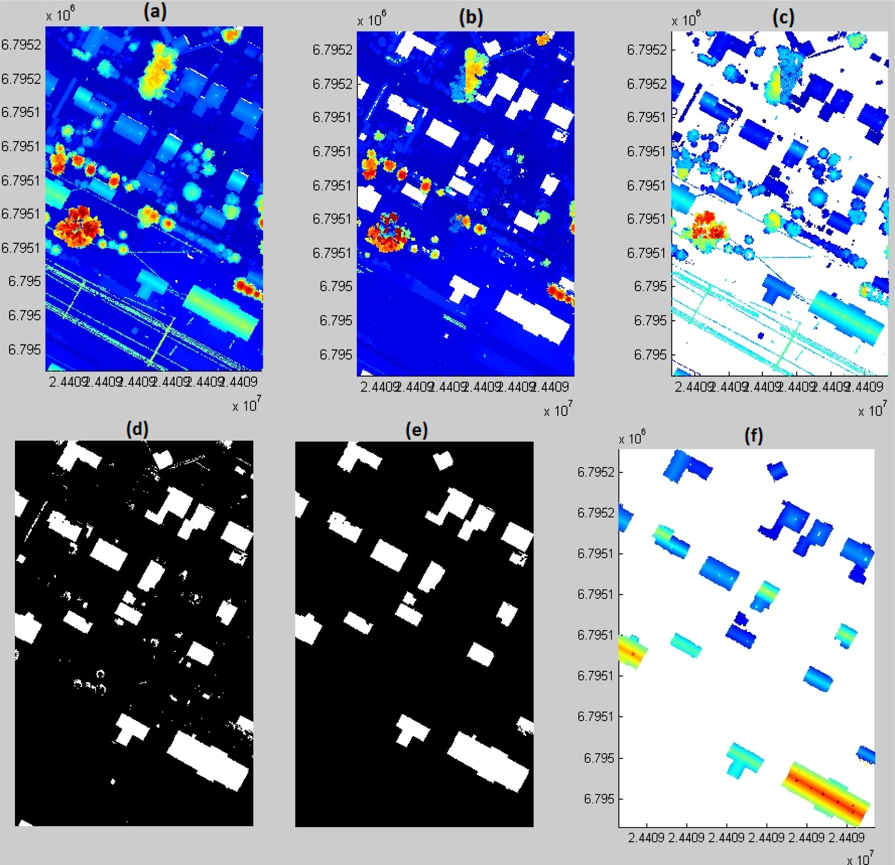
3.1.2. Building roofs

This paper proposes a simple and novel approach for building roof extraction from ALS. The algorithm is detailed below.

(i)

Grid the data and separate the data into two sub-datasets (processing the points grid by grid): Dlower and Dupper, where Dlower refers to the points that their height differences from the lowest point of the grid are less than or equal to 2.5 m, Dupper is the points that their height differences from the lowest point of the grid are less than 2.5 m.

(ii)

Transform Dlower (–xy plane view) into a binary image and accept objects as 0 and no objects as 1.

(iii)

Process the binary image and remove the noise points by thresholding the parameters of image processing, which are the area and shape of each region.

(iv)

Transform the cleaned binary image back to a 3D point cloud (the reverse process in step (ii)).

(v)

Construct the TIN to remove the scattered noise points.

(vi)

Utilize histograms to find the clusters and remove the small cluster points.

In the first step, we separate the data in n * n grids. For each grid, data are split into two height levels: Z_i − Z_min > 2.5 m and Z_i − Z_min ≤ 2.5 m, where Z_i is the height of a point and Z_min is the minimum height value in the grid. Thus, two sub-datasets are formed: Dlower and Dupper. Because of the characteristics of ALS (see Figure 7a), one laser pulse hits the building surface and produces one echo. Therefore, there are no laser hits on the bottom part of the building (see Figure 7b). Figure 7c shows the points which are at least 2.5 m higher than ground. Next, Dlower is transformed into a binary image according to the predefined pixel size. The binary image accepts a pixel as zero when there are objects located in the grid; otherwise, a pixel is 1. Figure 7d illustrates the derived binary image. From a visual interpretation, it contains not only buildings but also non-building points. Therefore, certain parameter constraints of regional properties are applied to the binary image processing so that the noise points can be properly removed. In the test data, the constraint parameters include “Area”, “MinorAxisLength”, “Eccentricity” and “Extent”, where “Area” refers to the actual number of pixels in the region; “MinorAxisLength” is the length (in pixels) of the minor axis of the ellipse that has the same normalized second central moments as the region; “Eccentricity” is the ratio of the distance between the foci of the ellipse and its major axis length; “Extent” is the ratio of pixels in the region to pixels in the total bounding box (the smallest rectangle containing the region). After image processing, the noise points are removed (Figure 7e), and the cleaned image is transformed back to a 3D point cloud (Figure 7f). However, it is still possible for certain noise points to be close to the detected buildings, and such points cannot be removed from images. For example, in the case of noise points above roofs, when all points are projected onto the –xy plane, the noise points, such as trees, above a building’s roof are overlapped with the roof in –xy plane or close to the edges of the roof. A triangulated irregular network (TIN) is then constructed, and the lengths of the edges are thresholded to remove the scattered noise points, and histograms are analyzed for the clusters. To remove the small cluster points, we analyze the histograms for different projections: xy plane, xz plane and yz plane.

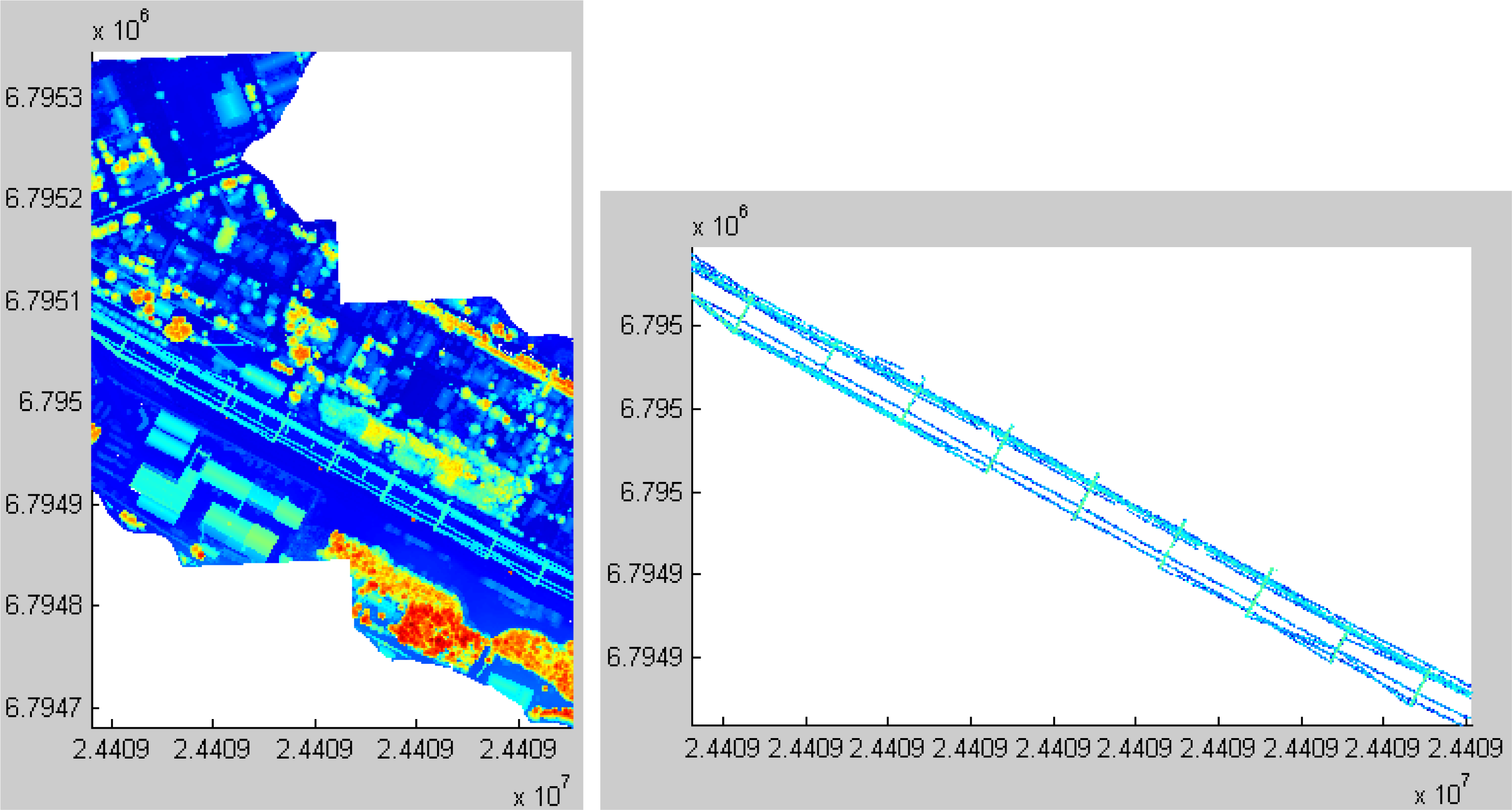
3.1.3. Powerlines

High-voltage powerlines play an important role in railway environments. Manual monitoring of powerlines is costly, time consuming and does not guarantee security. In recent decades, powerline data were mainly acquired by aerial images taken by manual or semi-automated methods. Currently, the ALS data with 49.62 points/m² offers detailed information for powerline modeling. The algorithm developed for ALS provides a fully automated method of modeling powerlines and detecting their elements. Figure 8 shows the ALS point cloud and extracted powerlines and racks.

In this paper, we propose an approach for classifying powerlines and pylons in railway environments. The focuses are primarily on the locations and heights of the pylons so that the 3D scene can be correctly modeled. The idea is that firstly according to the gradient (Fx, Fy) of each point, objects are separated. Objects with similar gradients form a group of points that are transformed into a binary image. The binary image is processed according to certain constraints of the image region properties, such as the region’s shape, length and area. Thus, the non-powerline objects are removed. Details for transforming and operating the binary images and removing the non-powerline objects can be found in Zhu et al. [8], which provides the details of a photorealistic building reconstruction from the MLS data. The steps of the algorithm are as follows:

(i)

Calculate the gradient for each point: $\text{Fx}=\frac{\partial \text{Z}}{\partial \text{x}}$, $\text{Fy}=\frac{\partial \text{Z}}{\partial \text{y}}$, where Z = F(x, y);

(ii)

Obtain points that satisfy the conditions: |Fx| ≥ T1 and |Fx| ≤ T2, and |Fy| ≥ T1 and |Fy| ≤ T2, where T1 < T2;

(iii)

Transform the 3D points into a 2D binary image and use the constraints in the image region properties to remove non-powerline related objects;

(iv)

Transform the derived powerline image into a 3D point cloud;

(v)

For pylon detection, grid the point cloud and count the number of points (Pcnt) in each grid; generate the binary image: when Pcnt ≥ T, label it as 1. Otherwise, label it as zero. T is the threshold for the number of the points.

(vi)

Transform the binary image back to a 3D point cloud for the resulting pylons.

(vii)

The heights and positions of the pylons are derived by calculating the height difference of each pylon and extracting the endings of each pylon.

Figure 9 shows the result of the pylon extraction from the ALS point cloud. The original point density has a significant influence on the results.

3.1.4. Trees

Trees are an important component of railway environments that add vitality to a 3D scene. Tree extraction from ALS has primary been focused on forest inventories. A summary of the methods used for forest inventory can be found in Hyyppa et al. [43]. A recent paper by Kaartinen et al. [44] on individual tree detection and extraction using ALS compared different methods and evaluated test areas with different point densities (2, 4, and 8 points per m²). The comparison was implemented internationally by 8 partners: Germany, Sweden, Finland, Norway, Taiwan, USA, Italy, and Switzerland. In addition to the comparison, four methods were implemented and tested by the Finnish Geodetic Institute (FGI): FGI_LOCM (local maxima detection), FGI_MLOG (multi-scale Laplacian of Gaussian filtering), FGI_MCV (minimum curvature-based tree detection) and FGI_VMS (local maxima detection with varying window size). After the comparison, the results showed that FGI_MCV and FGI_LOCM were among the best methods. FGI_MCV was based on the minimum curvature computation of the canopy height model (CHM), whereas FGI_LOCM first searches the local maxima in a given neighborhood and then delineates the tree crowns using marker-controlled watershed transformations from the tree locations, which are used as control markers. Finally, the tree locations and heights were achieved by finding the highest value within each tree segment. The results from those methods were more accurate than manual processing.

3.2. Object Extraction from MLS Point Cloud

3.2.1. Building Facades

The data collected by MLS are along railroads and extend for approximately 50 m on either side. However, MLS does not detect all of the buildings detected by ALS, which can be explained by the following reasons: (i) the buildings are too far from the scanner and (ii) dense trees in front of the buildings make the walls invisible. Figure 10 shows the process of building facade extraction. The building facades are extracted from the MLS data by using the method proposed in Zhu et al. [45]: data are analyzed by intercepting the different height passes to reduce the adhesions between buildings and trees. Based on the assumption that the walls are vertical to the ground (in a mapping ENU coordinate system, from the top view of the data, the building walls, which are vertical to the ground, are line-like. It means their x, y coordinates are clustered.), the planar coordinates of intercepted passes are compared and extract the points with same x, y coordinates in different passes for rough wall detection. These rough wall points are transformed into a binary image. Using image parameter constraints, the non-wall areas are removed and the image of the refined walls is transformed into 3D points. Figure 9 shows the results of building facade extraction.

3.2.2. Poles

Pole-like objects such as street lights or traffic signal lights are essential in road environments and especially in railway environments. MLS with 300,000 measurements per second provides detailed information for pole detection and modeling. A method for pole detection from MLS has been proposed [46] that employs the following strategy: (i) preprocessing the point cloud to make the pole feature more visible; (ii) transferring the preprocessed point cloud to a binary image without considering the height information; (iii) removal of the noise in the binary image by image processing technology; and iv) transferring the binary image without noise (iii) back to a point cloud (the reverse process of (i)). In this paper, pole detection was implemented but without statistical analysis. Therefore, it was not presented in the results.

3.3. Object Fusion and Building Planar Separation

3.3.1. Complete Building Models

Complete building models contain both building facades and roofs. From the previous steps, methods have been proposed to extract building roofs and facades from ALS and MLS data, respectively. The results from ALS and MLS provide complementary data. Figure 11 illustrates the process and results of data fusion. Because of dense points and high accuracy from both the ALS and MLS data, the building roofs are well-matched with the building facades. However, in the area of interest, additional roofs are visible compared to building facades. Therefore, complete building models are only achieved when both building facades and building roof are visible from both scanners (ALS and MLS) (Figure 12).

3.3.2. Planar Detection of Buildings

Because of the density of points from scanners, after complete buildings have been derived, there are still dense points presented as building points, which makes data post-processing, including model storage and rendering, less efficient. A 3D building model makes use of key points to represent the contours of a building and is a simplified version of all building points. To extract the key points, plane detection and separation are important.

Numerous algorithms have been developed for plane detection, such as RANSAC (random sample consensus), the Hough transformation, plane fitting, region growing, and clustering. These algorithms are usually based on a certain scene or several different scenes, and it is difficult to achieve a unified standard for any one scene. Therefore, researchers are continuously extending or updating old algorithms to solve existing problems. For example, the classical Hough transformation (also called 2D Hough transformation) is applied to an image to detect different features or shapes, such as lines, planes, circles and ellipses, by a voting implementation in the parameter space and then deriving the number of votes from an accumulator. When the number of votes in an accumulator’s bin is greater than a certain threshold, these points are extracted as the defined feature. Because 3D point clouds are widely utilized, 2D Hough transformation methods were then extended to 3D space. 3D Hough transformations for planar detection include the standard Hough transformation, adaptive probabilistic Hough transformation, progressive probabilistic Hough transformation and randomized Hough transformation (RHT) (Borrmann et al. [47]).

In this paper, the plane detection is performed by an improved method of RHT. In 3D laser point clouds, a plane can be defined as Z = axX + ayY + R, where X, Y, Z are the coordinates of a point, ax and ay are the slopes in the x- and y- direction, and R is the distance between a plane to the origin of the coordinate system. However, this method causes problems when the vertical plane is represented with infinite slope values. The equation R = XNx + YNy +ZNz, where Nx, Ny, and Nz are the components of the normal vector of a potential plane, was developed to avoid this problem. Each point votes for a sinusoidal surface, and their intersection indicates the presence of a plane. 3D Hough transformations have been proven effective for plane detection. However, the main drawback of this method is the computational cost, especially for dense laser point clouds. To reduce the computational cost, we employ RHT for plane detection with an initial value and a search range constraint. First, three points (p1, p2, p3) are selected randomly from the input data (building points) to define an initial plane. To make the algorithm more efficient, certain constraints are placed on the random initial points: (i) the distances between the points are less than 2 m; (ii) the three points are judged as being in a straight line or not, and only non-straight lines are used (new points are randomly selected if only straight lines are found); and (iii) for each point, their normals are calculated; if the normals are in similar directions, the selection of those initial points was a success; otherwise, new initial points are randomly generated again. This step increases the possibilities of plane detection and reduces the computational cost.

After the initial points are selected successfully, the normal vector of the defined plane is determined by:

$$N_x=\left|\begin{array}{lll}1\hfill & y_1\hfill & z_1\hfill \\ 1\hfill & y_2\hfill & z_2\hfill \\ 1\hfill & y_3\hfill & z_3\hfill \end{array}\right|,N_y=\left|\begin{array}{lll}{x}_1\hfill & 1\hfill & z_1\hfill \\ x_2\hfill & 1\hfill & z_2\hfill \\ x_3\hfill & 1\hfill & z_3\hfill \end{array}\right|,N_z=\left|\begin{array}{lll}{x}_1\hfill & y_1\hfill & 1\hfill \\ x_2\hfill & y_2\hfill & 1\hfill \\ x_3\hfill & y_3\hfill & 1\hfill \end{array}\right|.$$

The distance between the plane and the origin of the coordinate system is calculated as R = N × p1, where N = [Nx Ny Nz]. To reduce the calculation cost, the points located in the area from the center of the randomly selected points at approximately e.g., 35 m (the length of the longest roof edge in the dataset) are candidates for coplanar points for the Hough parameter calculation. The area of interest can also be defined according to the maximum size of the buildings in the dataset. The accumulator increases if |Rn − R| < T, where Rn = N × pn, T is the threshold. When the number of the accumulator is greater than a threshold, e.g., 50, the plane is extracted. After a plane is detected by using the Hough parameter accumulator, noise points may exist if the neighboring buildings are close and have the same slope of the planes (or the same normal vectors). Therefore, TIN is used to calculate the triangulation constraint for the final plane. After a plane is detected, those points are removed from the data. The above procedure is repeated until all points belong to a specific plane.

After plane detection, the intersection lines of the planes are calculated. Based on the intersection lines, the minimum box of each plane is obtained. According to the distances between the box corners and nearest laser points, the shape is adjusted. The final models can be created by meshing the extracted key points in each plane. Figure 13 shows the results of the building plane detection by using our improved RHT. Different colors in the figure represent the different planes.

3.4. Ground Model

Ground Model Simplification

After ground points are classified from the ALS data, the number of points is still extremely large. The dense ground points not only take up a significant amount of storage space, but they also result in low efficiency and expensive computational costs for data post-processing, e.g., surface meshing and model rendering. Therefore, the ground model must be simplified. Many different types of software offer a reasonable solution for automatic ground extraction from ALS, and the final products are commonly stored in raster format. Whether the terrain is flat or undulated, raster DEMs present the points with uniform spaces, which produces redundant points for flat terrain and inadequate representation in a changing or sloped area. To overcome this drawback, a quadtree algorithm is applied to simplify the ground model.

The quadtree algorithm was originally used for 2D data. Therefore, to employ this algorithm for 3D ground points, we must first transform the 3D points to a grey image with a size of 1024 × 1024, for example. The image size for a quadtree algorithm should be in 2n × 2n. The ground points are gridded by its X and Y coordinates according to the defined image size. The height value Z of each cell is derived from Z = f (X, Y). The intensity value for each pixel in the image is calculated by g(i, j) = Z(i, j) / Zmax, where g(i, j) denotes an intensity value / a grey value, Z(i, j) is the elevation of a point, and Zmax is the maximum elevation over the entire area. Thus, a grey image is formed, and the quadtree algorithm is conducted based on the grey image. The quadtree algorithm is a tree structure that recursively decomposes a square or rectangular into four quadrants or regions or sub-quadrants or sub-regions (Figure 14) according to predefined thresholds/criteria, e.g., 0.01. A grey value of 0.01 corresponds to the terrain elevation with a value of 0.01 × Zmax. Therefore, the height difference in the final sub-quadrants or sub-regions meets the predefined criteria. For our study, we may set different thresholds / criteria to acquire different levels of detail of the ground model. The simplified model still retains the primary terrain characteristics, but the size of the model is greatly reduced by up to 99.36% of the original data. In next section, the method will be analyzed and discussed.

4. Results and Discussion

The methods presented above have been applied for the area around the railway station of Kokemaki, Finland. The test data covers an area with a length of approximately 1000 m and a width of approximately 100 m (both ALS and MLS are visible). The resulting 3D scene (Figure 15) includes the ground, buildings, and powerline pylons. The geometry of the ground and buildings and the parameters of the pylons and powerlines were derived from the algorithms presented in this paper. Orthophoto was utilized for the ground texture and visual analysis. The software 3Ds Max was employed for the final model visualization.

The validation of the algorithms was implemented by visually comparing the classified results to the orthophoto with a ground resolution of 20 cm (Figure 16).

Table 1. Evaluation of the results.

Statistical Items	The Number of Objects on the Orthophoto	The Number of Objects from the Point Cloud	Detection Accuracy
Buildings from ALS	61	57	93.44%
Walls from MLS	10	10	100%
Powerline pylons	20	20	100%

lists the comparison results between the detected objects and objects on the orthophoto and the accuracy of the detection algorithms.

4.1. Building Classification Results

The validation was implemented based on data from the test area. Figure 16 shows the test area from the orthophoto and the result of the building classified from ALS. The algorithms proposed in Section 3 have been applied to the test data. Table 1 shows that 57 out of 61 buildings were detected from the ALS data. Two buildings were missing because of their small size. When the binary image was filtered during building detection, the parameter “area” was adjustable. If smaller thresholds had been applied, all buildings could have been detected; however, small noise/non-building objects would probably have been misclassified as buildings and resulted in redundant buildings. Therefore, the selection of thresholds had a significant influence on the results. For the test field, the total accuracy in building roof detection was 93.44%. In the MLS data, only a few building facades were presented because (i) the available data were limited to 50 m away from the driving direction and (ii) the buildings were obstructed by trees. The building facades were successfully detected from the MLS data by using the method proposed by Zhu et al. [46]. When utilizing MLS data for successful building wall extraction, the test area should be selected based on a low amount of tree obstructions and reflective objects. Our test area was around a railway station, and the buildings were clearly visible from the scanners, which indicated the feasibility of reconstructing railway stations from MLS and ALS data.

4.2. Powerlines and Pylons

The desired result for powerlines and pylon detection was achieved in the test area primarily because of the (i) dense point cloud and (ii) clear cutoff edges between powerlines and trees. These two requirements were essential for the algorithm. The density of the point cloud was particularly important for pylon detection. In our algorithm, the number of points was accumulated and the threshold was set for pylon detection. In the majority of cases, powerlines are located at a distance away from the surrounding trees and forests. Therefore, the algorithm was appropriate for areas that satisfied the above requirements.

4.3. Ground Model Simplification

The quadtree algorithm developed for model simplification not only greatly reduces the original data size, but it also retains the original terrain features. By using this algorithm, the data size can decrease by up to 0.64% of the original data size (

Table 2. Ground model simplification evaluation.

	Number of Original Points	Number of Points after Simplification	Reduction Rate
0.005	6,890,129	252,339	96.34%
0.01		181,232	97.37%
0.02		113,165	99.36%

). This algorithm is flexible and enables users to select the level of detail of the ground according to different applications. Figure 17 shows how the parameter selection affects the resulting models. The main parameter in the quadtree algorithm is the criteria of the sub-quadrants or sub-regions. Smaller parameters include more ground detail information.

Table 2 shows an example of different parameter values corresponding to the number of points after simplification and the reduction rate.

Reduction rate = (number of original points − current number of points)/number of original points

The number of original points was 6,890,129. The massive amount of original ground points could present a challenge for the post-processing of the model. Our algorithm produced an effective method of reducing the data size that preserves the original features. When the criterion of the sub-quadrants was set to 0.005, the number of points was reduced by 96.34%, which represented a well-defined ground surface. The run time of the algorithm was 51.47 seconds based on the number of points (6,890,129).

The ALS and MLS systems have different scan geometries and provide different point densities as well as different data resolutions. We made full use of the different advantages from ALS and MLS in the 3D modeling process. Both data render complementary characteristics, especially for buildings. For instance, MLS shows the building facades in detail but is not able to provide complete building contours. ALS has a large area and provides details for roofs but not building facades. Powerlines and pylons can be detected from both datasets if ALS provides enough dense points (in our case, 50 points/m²). However, accurate MLS data have a range limitation of approximately 50 m from the target. If the directions of powerlines are not along corridors or are out of view of the MLS system, then complete powerline modeling from MLS is difficult; therefore, MLS modeling of powerlines is dependent on the local environment and data quality. In this paper, we developed the algorithm from only the ALS data. For the poles, we would recommend using MLS data for modeling detailed geometry.

Further work will test the data from different environments. As we know, railway environments are complex. The terrain varies from flat areas to mountain areas. The surroundings of railway environments can also include tunnels and viaducts and so on. The complexity of 3D modeling in those areas will greatly increase. Therefore, further studies in that kind of areas are needed.

5. Conclusions

This paper addressed modeling an entire railway environment that contained objects such as the ground, railroads, buildings, powerlines and pylons, street / traffic lights, and trees by using both MLS and ALS datasets. New solutions were proposed for object extraction, 3D reconstruction, model simplification and final model 3D visualization based on image processing technology for classification, 3D randomized Hough transformations (RHT) for planar detection, and a quadtree approach for ground model simplification. Some basic conclusions are as follows:

(i)

An entire railway environment was successfully reconstructed from ALS and MLS datasets.

(ii)

Automatic algorithms for modeling buildings from both ALS and MLS data were developed. The accuracy of building detection from ALS is 93.44% for the test data.

(iii)

Powerlines and pylons were extracted from ALS data. An acceptable result was achieved because of the dense point cloud and clear cutoff edge between the powerlines and surrounding environments.

(iv)

An algorithm for ground model simplification has been proposed. The reduction of points was up to 99.36% of the original point size, which was beneficial for model post processing and 3D visualization. It was especially flexible because users can select the level of ground detail in different applications.

References

- Railways and the Environment: Building on the Railways’ Environmental Strengths. Available online: http://www.cer.be/publications/brochures/brochures-details/railways-and-the-environment-building-on-the-railways-environmental-strengths/ (accessed on 7 February 2014).
- Railway Passenger Transport Industry: Market. Research Reports, Statistics and Analysis. Available online: http://www.reportlinker.com/ci02334/Railway-Passenger-Transport.html (accessed on 16 August 2013).
- RIEGL Website. Available online: http://www.riegl.com/ (accessed on 21 January 2014).
- Kukko, A.; Kaartinen, H.; Hyyppa, J.; Chen, Y. Multiplatform mobile laser scanning: Usability and performance. Sensors 2012, 12, 11712–11733. [Google Scholar]
- Model-Driven and Data-Driven Approaches Using Lidar Data: Analysis and Comparison. Available online: http://www.pf.bgu.tum.de/isprs/pia07/puba/PIA07_Tarsha-Kurdi_et_al.pdf (accessed on 7 February 2014).
- 3D City Map Website. Available online: http://www.computamaps.com/products/3Dcitymap.htm (accessed on 20 Noveber 2013).
- Wang, R. 3D building modeling using images and LiDAR: A review. Int. J. Image Data Fusion 2013, 4, 273–292. [Google Scholar]
- Hyyppa, J.; Zhu, L.; Liu, Z.; Kaartinen, H.; Jaakkola, A. 3D City Modeling and Visualization for Smart Phone Applications. In Ubiquitous Positioning and Mobile Location-Based Services in Smart Phones; Chen, R., Ed.; Chapter 10; IGI Global: Hershey, PA, USA, 2012. [Google Scholar]
- Baltsavias, E.P. Object extraction and revision by image analysis using existing geodata and knowledge: Current status and steps towards operational systems. ISPRS J. Photogramm. Remote Sens 2004, 58, 129–151. [Google Scholar]
- Brenner, C. Building reconstruction from images and laser scanning. Int. J. Appl. Earth Obs. Geoinf 2005, 6, 187–198. [Google Scholar]
- Kaartinen, H.; Hyyppa, J. EuroSDR-Project Commission 3 “Evaluation of Building Extraction”, Final Report; No. 50; EuroSDR Official Publication: Leuven, Belgium, 2006. [Google Scholar]
- Haala, N.; Kada, M. An update on automatic 3D building reconstruction. ISPRS J. Photogramm. Remote Sens 2010, 65, 570–580. [Google Scholar]
- Automatic Extraction of Vertical Walls from Mobile and Airborne. Available online: http://www.isprs.org/proceedings/xxxviii/3-w8/papers/p74.pdf (accessed on 7 February 2014).
- Extraction and Modeling of Powerlines from ALS Point Clouds. Available onlne: http://www.ipf.tuwien.ac.at/cb/publications/melzer_powerlines_OAGM_2004.pdf (accessed on 7 February 2014).
- McLaughlin, R.A. Extracting transmission lines from airborne LIDAR Data. IEEE Geosci. Remote Sens Lett 2006, 3, 222–226. [Google Scholar]
- Automatic 3D Powerline Reconstruction Using Airborne Lidar Data. Available online: http://www.isprs.org/proceedings/xxxviii/3-w8/papers/p105b.pdf (accessed on 7 February 2014).
- Automatic Powerline Scene Classification and Reconstruction Using Airborne Lidar Data. Available online: http://www.isprs-ann-photogramm-remote-sens-spatial-inf-sci.net/I-3/167/2012/isprsannals-I-3-167-2012.pdf (accessed on 7 February 2014).
- Extraction of Features from Mobile Laser Scanning Data for Future Driver Assistance System Advances in GIScience. Available online: http://link.springer.com/chapter/10.1007%2F978-3-642-00318-9_2 (accessed on 7 February 2014).
- Shape-Based Recognition of 3D Point Clouds in Urban Environments. Available online: http://www.cs.princeton.edu/~funk/iccv09.pdf (accessed on 7 February 2014).
- Lehtomaki, M.; Jaakkola, A.; Hyyppa, J.; Kukko, A.; Kaartinen, H. Detection of vertical pole-like objects in a road environment using vehicle-based laser scanning data. Remote Sens 2010, 2, 641–664. [Google Scholar]
- Pu, S.; Rutzinger, M.; Vosselman, G.; Elberink, S.O. Recognizing basic structures from mobile laser scanning data for road inventory studies. ISPRS J. Photogramm. Remote Sens 2011, 66, 28–39. [Google Scholar]
- Optimizing Detection of Road Furniture (Pole-Like Object) in Mobile Laser Scanner Data. Available online: http://www.itc.nl/library/papers_2013/msc/gfm/danli.pdf (accessed on 7 February 2014).
- Hay, G.J.; Castilla, G. Geographic Object-Based Image Analysis (GEOBIA). In Object-Based Image Analysis—Spatial Concepts for Knowledge-Driven Remote Sensing Applications; Blaschke, T., Lang, S., Hay, G. J., Eds.; Chapter 1.4; Springer: Verlag, Berlin, Germany, 2008; pp. 81–92. [Google Scholar]
- Nussbaum, S.; Menz, G. Object-Based Image Analysis and Treaty Verification: New Approaches in Remote Sensing—Applied to Nuclear Facilities in Iran; Springer Verlag: Berlin, Germany, 2008. [Google Scholar]
- Blaschke, T. Object based image analysis for remote sensing. ISPRS J. Photogramm. Remote Sens 2010, 65, 2–16. [Google Scholar]
- Clode, S.; Rottensteiner, F.; Kootsookos, P.; Zelniker, E. Detection and vectorisation of roads from LIDAR data. Photogramm. Eng. Remote Sens 2007, 73, 517–535. [Google Scholar]
- Assessing Image Segmentation Quality—Concepts, Methods and Application. Available online: http://www.isprs.org/proceedings/xxxviii/4-c1/sessions/Session2/6721_Neubert_Proc_pap.pdf (accessed on 7 February 2014).
- Boyko, A.; Funkhouser, T. Extracting roads from dense point clouds in large scale urban environment. ISPRS J. Photogramm. Remote Sens 2011, 66, S2–S12. [Google Scholar]
- Dong, J.; Zhuang, D.; Huang, Y.; Fu, J. Advances in multi-sensor data fusion: Algorithms and applications. Sensors 2009, 9, 7771–7784. [Google Scholar]
- Beger, R.; Gedrange, C.; Hecht, R.; Neubert, M. Data fusion of extremely high resolution aerial imagery and LIDAR data for automated railroad center line reconstruction. ISPRS J. Photogramm. Remote Sens 2011, 66, S40–S51. [Google Scholar]
- An Integrated On-Board Laser Range Sensing System for On-The-Way City and Road Modeling. Available online: http://www.isprs.org/proceedings/xxxvi/part1/Papers/T10-43.pdf (accessed on 7 February 2014).
- Kukko, A. Road Environment Mapper—3D Data Capturing with Mobile Mapping. Licentiate’s Thesis, Helsinki University of Technology, Espoo, Finland,. 2009; 158. [Google Scholar]
- Jaakkola, A.; Hyyppa, J.; Hyyppa, H.; Kukko, A. Retrieval algorithms for road surface modeling using laser-based mobile mapping. Sensors 2008, 8, 5238–5249. [Google Scholar]
- Zhou, Q.; Chen, Y. Generalisation of DEM for terrain analysis using a compound method. ISPRS J. Photogramm. Remote Sens 2011, 66, 38–45. [Google Scholar]
- VR Track Oy Website. Available online: http://www.vrgroup.fi/en/ (accessed on 7 February 2014).
- Yu, X.; Hyyppa, J.; Vastaranta, M.; Holopainen, M.; Viitala, R. Predicting individual tree attributes from airborne laser point clouds based on random forests technique. ISPRS J. Photogramm 2011, 66, 28–37. [Google Scholar]
- Kraus, K.; Pfeifer, N. Determination of terrain models in wooded areas with aerial laser scanner data. ISPRS J. Photogramm. Remote Sens 1998, 53, 193–203. [Google Scholar]
- DEM Generation from Laser Scanner Data Using Adaptive TIN Models. Available online: http://www.isprs.org/proceedings/xxxviii/7-C4/308_GSEM2009.pdf (accessed on 7 February 2014).
- Raber, G.T.; Jensen, J.R.; Schill, S.R.; Schuckman, K. Creation of Digital Terrain Models using an adaptive Lidar vegetation point removal process. Photogramm. Eng. Remote Sens 2002, 68, 1307–1316. [Google Scholar]
- Ma, R.; Meyer, W. DTM generation and building detection from Lidar data. Photogramm. Eng. Remote Sens 2005, 71, 847–854. [Google Scholar]
- Shan, J.; Sampath, A. Urban DEM generation from raw LiDAR data: A labeling algorithm and its performance. Photogramm. Eng. Remote Sens 2005, 71, 217–226. [Google Scholar]
- Meng, X.; Currit, N.; Zhao, K. Ground filtering algorithms for airborne Lidar data: A review of critical issues. Remote Sens 2010, 2, 833–860. [Google Scholar]
- Hyyppa, J.; Hyyppa, H.; Leckie, D.; Gougeon, F.; Yu, X.; Maltamo, M. Review of methods of small footprint airborne laser scanning for extracting forest inventory data in boreal forests. Int. J. Remote Sens 2008, 29, 1339–1366. [Google Scholar]
- Kaartinen, H.; Hyyppa, J.; Yu, X.; Vastaranta, M.; Hyyppa, H.; Kukko, A.; Holopainen, M.; Heipke, C.; Hirschmugl, M.; Morsdorf, F.; et al. An international comparison of individual tree detection and extraction using airborne laser scanning. Remote Sens 2012, 4, 950–974. [Google Scholar]
- Zhu, L.; Hyyppa, J.; Kukko, A.; Kaartinen, H.; Chen, R. Photorealistic 3D city modeling from mobile laser scanning data. Remote Sens 2011, 3, 1406–1426. [Google Scholar]
- The Use of Mobile Laser Scanning Data and Unmanned Aerial Vehicle Images for 3D Model Reconstruction. Available online: http://www.int-arch-photogramm-remote-sens-spatial-inf-sci.net/XL-1-W2/419/2013/isprsarchives-XL-1-W2-419-2013.pdf (accessed on 7 February 2014).
- The 3D Hough Transform for Plane Detection in Point Clouds—A Review and A new Accumulator Design. Available online: http://link.springer.com/article/10.1007%2F3DRes.02%282011%293 (accessed on 7 February 2014).