Window Regression: A Spatial-Temporal Analysis to Estimate Pixels Classified as Low-Quality in MODIS NDVI Time Series

Abstract

MODerate resolution Imaging Spectroradiometer (MODIS) data are largely used in multitemporal analysis of various Earth-related phenomena, such as vegetation phenology, land use/land cover change, deforestation monitoring, and time series analysis. In general, the MODIS products used to undertake multitemporal analysis are composite mosaics of the best pixels over a certain period of time. However, it is common to find bad pixels in the composition that affect the time series analysis. We present a filtering methodology that considers the pixel position (location in space) and time (position in the temporal data series) to define a new value for the bad pixel. This methodology, called Window Regression (WR), estimates the value of the point of interest, based on the regression analysis of the data selected by a spatial-temporal window. The spatial window is represented by eight pixels neighboring the pixel under evaluation, and the temporal window selects a set of dates close to the date of interest (either earlier or later). Intensities of noises were simulated over time and space, using the MOD13Q1 product. The method presented and other techniques (4253H twice, Mean Value Iteration (MVI) and Savitzky–Golay) were evaluated using the Mean Absolute Percentage Error (MAPE) and Akaike Information Criteria (AIC). The tests revealed the consistently superior performance of the Window Regression approach to estimate new Normalized Difference Vegetation Index (NDVI) values irrespective of the intensity of the noise simulated.

1. Introduction

The MODIS sensor (MODerate resolution Imaging Spectroradiometer) can be considered as a landmark in the technological and scientific advances for global, regional and local analysis, and acquisition and monitoring of phenomena related to atmosphere, oceans, and terrestrial surface [1]. The MODIS sensor stands out for its high temporal resolution, moderate spatial resolution and diverse spectral bands ranging from visible to thermal infrared. Additionally, the availability of its products favors several applications for mapping and monitoring the terrestrial surface [2].

Among the MODIS Land products, the MODIS Vegetation Index (MOD13) is of particular interest for vegetation phenology research. It comprises the Normalized Difference Vegetation Index (NDVI) and Enhanced Vegetation Index (EVI). The MOD13 includes products according to the acquisition data period and spatial resolution. For example, MOD13Q1 is composed of vegetation indices with a spatial resolution of 250 m and 16-day compositions [3].

Several authors [4–6] have reported that vegetation phenology can be observed, analyzed, and mapped by using a vegetation index (VI) time series. However, in [7,8], they show that the noises caused by different atmospheric conditions or by bidirectional effects related to the geometry of data acquisition pose some problems for the temporal profile analysis. These problems must be minimized before using the vegetation index temporal profile.

Part of the noises in time series can be removed through processing methods, including the Maximum Value Composite—MVC [9], during the composition of the time series. Nevertheless, the atmospheric disturbance cannot be removed effectively, especially in areas with high incidence of clouds. Therefore, several research groups have implemented or are still developing methods for filtering noises or reconstructing the time series to obtain data with better quality [10].

Numerous methodologies have been used for reducing noises in the time series of vegetation indices before the use of data for the estimation of vegetation phenological characteristics. The techniques cited in the literature include 4253H filter [11], Savitzky–Golay [12,13], Mean Value Iteration [7], weighted least squares regression approach [14], best index slope extraction [15], Whittaker smoother [10,16], and double logistic [17,18]. Other filtering techniques use harmonic analysis [5], Fourier analysis [19,20], or wavelet [6,21–23] for reducing noises in time series. The geostatistics approach has been used for filling out the gaps or the absence of data due to the presence of clouds [24–26]. Techniques that use spatial-temporal interpolation for pixel reconstruction [27–29] are also applied.

In general, various filtering techniques work in the frequency or temporal domain, i.e., they analyze the spectral behavior of the pixel in one domain of the information. These techniques are intended to reduce the noises and maintain the integrity of the VI for a satellite image time series. However, they do not consider the spatial and temporal correlation of the pixel values. The spatial-temporal interpolation method has to be flexible and able to provide reconstructed images reproducing spatial patterns and local features of the product analyzed [28,29]. Meanwhile, the quality information available on the MODIS products contributes to the appropriate interpretation and application, while the products considered as of low quality must be used with caution [30]. Therefore, the present study aimed to propose and to test a time series approach for estimating pixel values that have been classified as of low quality. As such, an estimation of new values will be based on regression analysis between only cloud-free data of optimal quality selected by binary MODIS Quality Assurance flags.

In this study, the analysis will be carried out with simulated data in order to evaluate the effectiveness of the proposed approach, which is the reduction of the noise of a single date or noises distributed over the time in a set of images. In addition to the evaluation related to noise distribution in space and in time, it also simulates and evaluates the efficiency of the noise intensity applied on a data.

2. Quality Assessment

The validation of the products obtained from the data provided by the MODIS sensor is based on methods that compare the information collected on test areas or the data acquired by other sensors. The MODIS Land (MODLAND) Science Team (ST) has been developing and coordinating activities to assess and validate the performance of the MODLAND products by incorporating the generated metadata to the quality data of each pixel in each product [3]. This quality information, which is called Quality Assessment (QA), allows the MODIS database users to verify the reliability of a pixel in relation to the atmospheric conditions (presence of clouds, ozone, dust, and other aerosols), and to check the bidirectional effects related to the geometry of the data acquisition (source-target-sensor) and the possible failures of instrumental or data processing methods [30].

The MODIS VI product suite has a set of output parameters for each pixel, known as Science Datasets (SDS), which comprises the following information: (1) composited NDVI and EVI; (2) quality of the information available (QA); (3) reflectance in bands 1, 2, and 7 (620–670 nm, 841–876 nm and 2105–2155 nm, respectively); (4) sensor zenith view angle, solar zenith angle, and relative azimuth; (5) day of the year on which the pixel was obtained; and (6) pixel reliability [31].

The QA images have bit values that document the conditions by which each pixel has been acquired and processed. Thus, pixel reliability is useful in post processing analysis and summarizes the QA status of the product. This parameter is a simple decimal number that ranks the product into five categories (Fill/No Data–Good Data–Marginal Data–Snow/Ice–Cloudy). Users can consult this information instead of working with the QA layer [32].

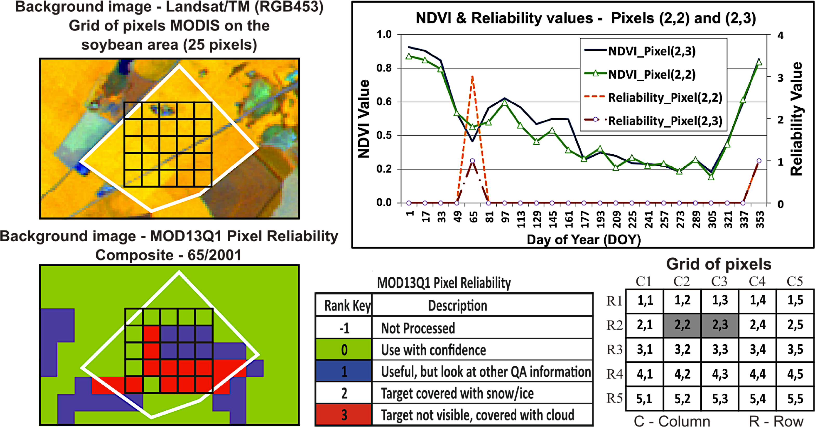
The need for the analysis of a set of VI values and the reliability of the pixel along the temporal profile is illustrated in Figure 1. It can be observed that the two-neighbor pixels present different reliability and NDVI values (proceeding from the same product MOD13Q1—MODIS/Terra Vegetation Indices-16 days-250 m) for the same composite date, land use, and land cover.

The difference in NDVI values between the neighboring pixels presented in Figure 1 can be related only to the vegetation spectral response. However, the QA values indicate that the conditions for the acquisition and processing of pixels were not the same. As it is known that the analyzed pixels (Pixel 2,2 and 2,3 from Figure 1) have the same type of land use and cover and development stages, the spectral responses between pixels were expected to be similar. Nevertheless, this has not been observed for all data along the NDVI time series, e.g., for the date 65, the (2,2) pixel was 23% higher than the (2,3) pixel.

3. Methodology

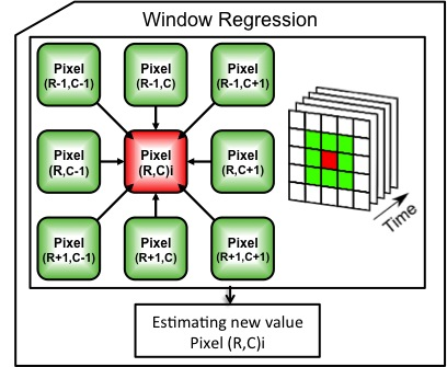
This research work aims to analyze noise reduction in NDVI time series, based on a simultaneous evaluation of the values from vegetation indices along time and space, including the pixel-level quality indicators provided with each MODIS land product. This contextual analysis assumes that terrestrial surface targets are related to each other. However, the neighboring targets are more related to each other than those separated by longer distances.

The method proposed to reconstruct the MODIS NDVI time series is divided into two steps: (A) the first step comprises a descriptive analysis of the time series, which is based on the quality information of the MOD13Q1 product. Information about pixel reliability, quality of vegetation indices, acquisition date and view geometry angles are useful for the arrangement and data selection. It will allow the construction of a mask that comprises the pixels (R,C)i (R-row, C-column, for a date i) classified as of low quality; (B) and the second step comprises a linear regression analysis based on a spatial-temporal window for recalculating the NDVI values of the pixels considered as of low quality. This estimate is based on the neighboring values of guaranteed quality (or pixels not named on the mask).

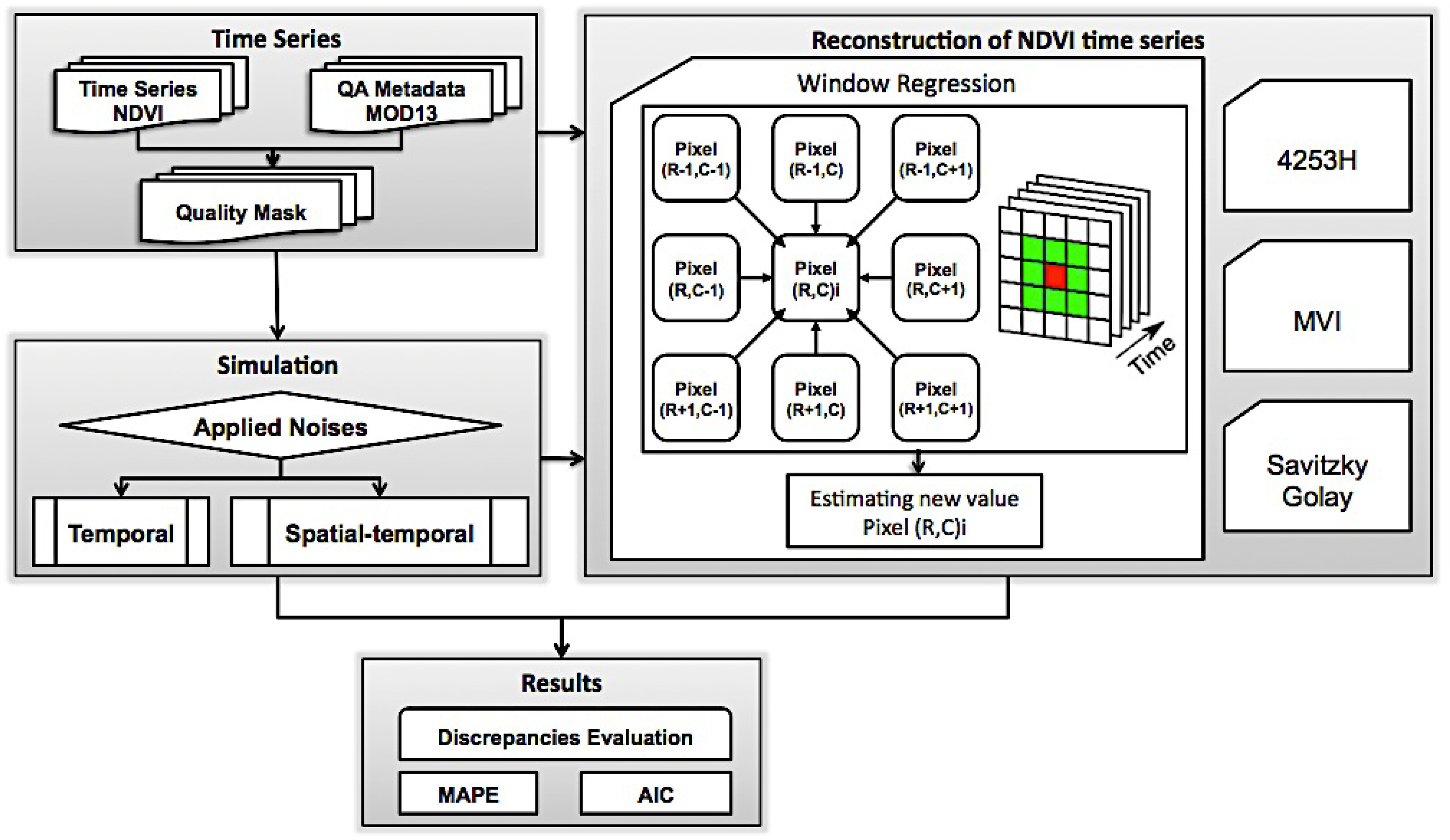
The steps for the implementation of the window regression technique, simulation data, and analysis of the results are illustrated in Figure 2.

3.1. Quality Mask and Spatial-Temporal Window Analysis of the Pixel (R,C)i

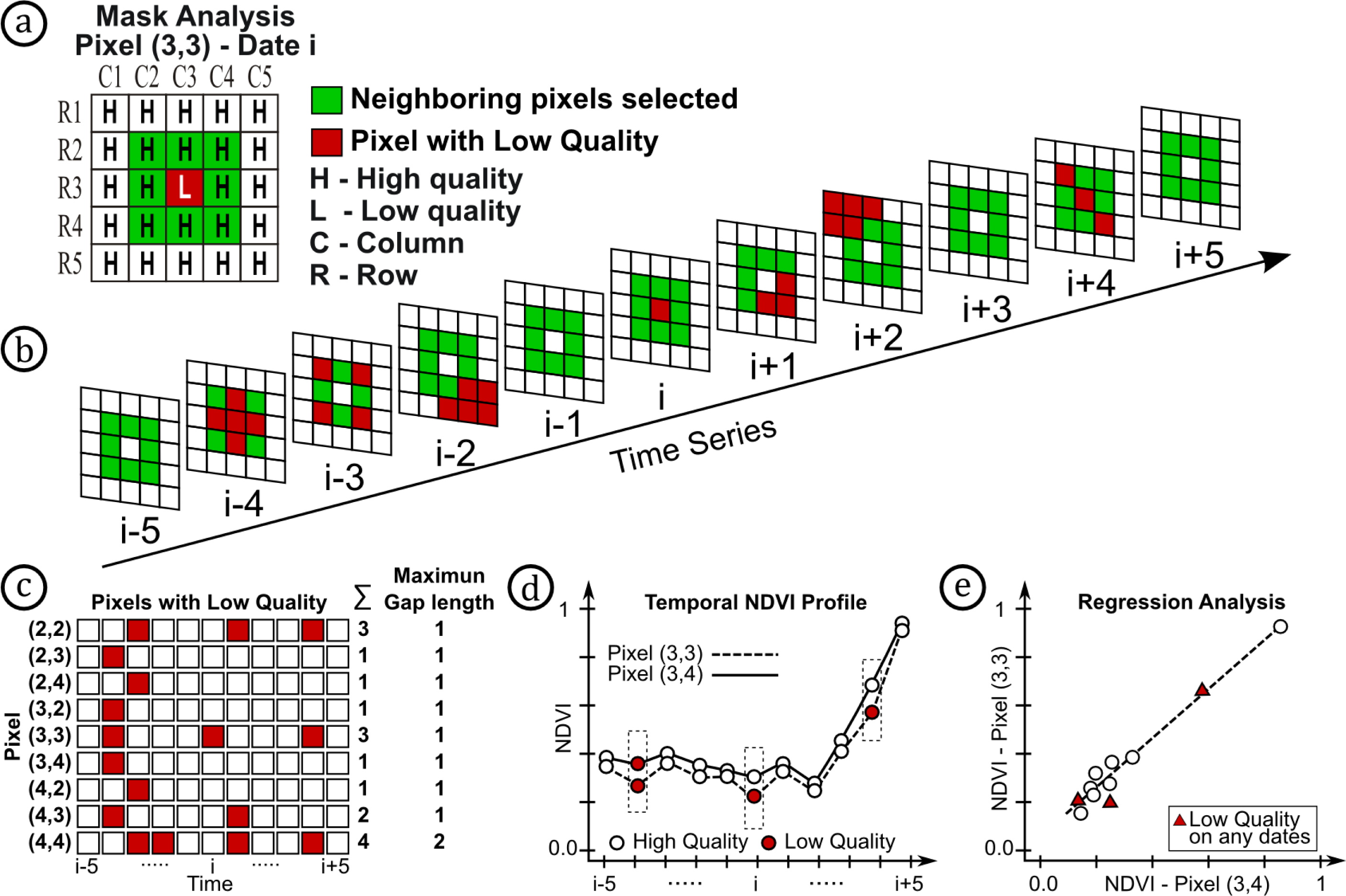
The first step of this method consists of the classification and selection of pixels of low quality from the MODIS products. In this study, the mask of the low quality pixels was composed of all pixels from the time series classified in the cloudy category. The pixel (3,3)i (line 3, column 3, data “i”), shown in Figure 3a, is included in the quality mask because it has been classified as of low quality. This pixel will be used as an example for estimating a new value from the time series approach suggested in this work. Next, an analysis window is defined, in time and space, to acquire the NDVI pixels and to compose the regression analysis.

The quality of the pixels along the NDVI time series may vary due to atmospheric condition changes and the variable illumination and viewing geometry at the moment of image acquisition. Thus, for each date prior to or after the date of interest (or date “i”), the spatial-temporal window selects only pixels that have been classified as of high quality by the metadata of the NDVI/MODIS product (Figure 3b). The spatial-temporal window construction starts with the verification of the quality parameters of the 8 pixels neighboring the pixel of interest, and only the pixels with high quality will be included in the data for the regression analysis.

The temporal window in this method aims to use the temporal profile comprised in the date prior to and after the data analysis. Therefore, this temporal analysis evaluates a set of NDVI values for a gap equivalent to 11 dates. Thus, for a pixel of interest (e.g., pixel (3,3)i), the temporal window analysis will be applied for the dates between “i − 5” and “i + 5”.

According to [33], the number of invalid pixels and the gap length to be interpolated on a temporal profile affect the estimation of new data. The amount of the inapt data is represented by the useful data for the entire length of the time series. The gap size considers the larger interval represented by invalid data sequences along the time. The combination of the spatial-temporal window and the quality mask for a pixel of interest allows estimating the amount of data considered inapt and the size of the gap for each neighboring pixel. This result is illustrated in Figure 3c.

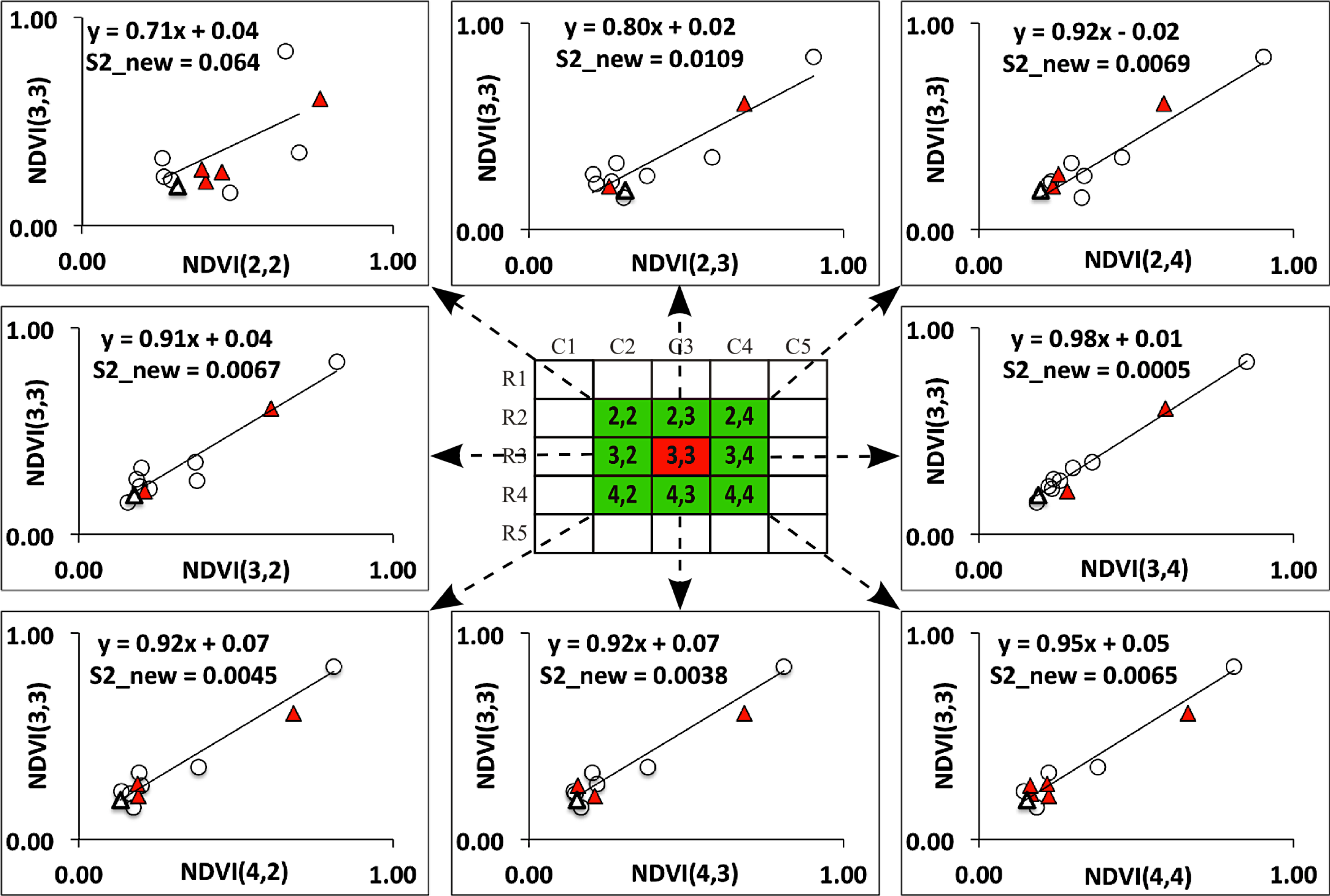
The newer values of the pixel (3,3)i will be provided by the regression analysis between the spatial-temporal window of the pixel of interest. Figure 3d illustrates a temporal profile of the pixel of interest with one of its neighbors. It shows the data that had been considered invalid by the mask previously applied. Amongst the pre-defined methodology criteria to compose the regression analysis, it is necessary to select the pairs of data considered apt, i.e., the data on both dates must be classified as of high quality. Thus, the example in Figure 3d shows that, on the three dates, the pair of data will not be used in the regression analysis because it was considered invalid at least in one of the pixels.

3.2. Linear Regression and Estimation of a New Value

The function that relates two variables may be expressed by the formula Y = f(X), where “Y” is the dependent variable and “X” is the independent variable. Considering a predictor variable and a linear function, the model can be described as follows:

$${\text{y}}_{\text{i}}={\beta }_0+{\beta }_1{\text{x}}_{\text{i}}+{\varepsilon }_{\text{i}}$$

(1)

where y_i is the value of the response variable in the observation “i”; β₀ and β₁ are parameters; x_i is the predictor in the observation “i”; and ɛ_i is the random error term. The least square methods can be used to obtain the estimators in the regression [34].

In the present study, the dependent variable is attributed to the selected data set for the pixel of interest (pixel (R,C)i). The independent variables are constituted of the data of the pixels close to the point to be estimated. It is important to emphasize that the value of a pixel considered inapt by the quality criteria is not used in the regression.

Figure 3e illustrates the dispersion diagram between the dependent and independent variables (temporal profile of the pixels (3,3) and (3,4)) together with the linear relation among the data considered as valid.

The value of the pixel of interest is excluded from the regression analysis since it is classified as invalid, according to the quality criteria. However, an estimation for a new value for this pixel (pixel (R,C)i) is considered as a new observation (Ynew) of the dependent data set. Likewise, the value of the independent variable used to estimate Ynew is represented by the neighboring pixel (R,C)i called Xnew. Ynew will deviate from the estimated mean of the response variable based on the original n observations in the study, and this difference may be viewed as the prediction error.

According to [34], an unbiased estimator of a variance of a data set with the inclusion of Xnew is expressed by:

$${\text{s}}_{\text{new}}^2=\text{MSE}\times \left[1+\frac{1}{\text{n}}+\frac{{\left({\text{X}}_{\text{new}}-\overline{\text{X}}\right)}^2}{{\sum }_{\text{i}=1}^{\text{n}}{\left({\text{X}}_{\text{i}}-\overline{\text{X}}\right)}^2}\right]$$

(2)

where ${\text{s}}_{\text{new}}^2$ is the variance of a data after the new element is included; MSE is the mean square error; n is the total of observations; Xnew is the new element of the independent variable; X is the independent variable; X is the average of X.

All the regression analysis proposed in this methodology was carried out based on the following criteria: (I) Only pairs of data considered valid or classified as of a good quality are used when the quality information of the MODIS product is consulted; (II) At least four pairs of valid data are used for the regression analysis, where at least two pairs of the data must be included into the periods prior to and after the date of interest; (III) The lower variance for a data set provides the regression model with a minimized sum of absolute deviations and, consequently, the estimated values present a lower error rate. Hence, the regression model equation that provides lower variance between all the possible regression analyses is classified as the best fit for the data set analyzed. Thus, it will be used to recalculate a new value for the pixel of interest.

This process to calculate the new value for the pixel (R,C)i is iterative. If the criteria II is not reached, the pixel is then maintained in the invalid data list, so it can be analyzed later. Figure 4 exemplifies all the possible regression analyses for all the neighboring pixels of the pixel (3,3)i. According to the pre-established selection criteria by the spatial-temporal window, as well by the variance analysis of the data set, the linear regression obtained between the pixels (3,3) and (3,4) will be used at the end of this process to estimate the data of interest.

3.3. Window Regression—Estimation of NDVI Values

The method for estimating the NDVI values of the pixels classified as of low quality will be named in this work as Window Regression (WR). The approach proposed for noise reduction is based on the regression analysis of the data selected by spatial-temporal window. The following procedure is conducted:

• Elaboration of a mask with pixels and data classified as of low quality, i.e., points that must have the NDVI recalculated.
• A random selection of all the pixels classified as of low quality is conducted prior to the regression analysis. This procedure aims to reduce the effect of a sequential analysis of the neighboring pixels classified as of low quality on the estimation of new VI values.
• After selecting the pixel (R,C)i, the reconstruction methodology of a new value uses regression analysis as previously described in topic 3.2.
• The estimated value for the pixel (R,C)i is apt to be used in another regression analysis. This is why the process returns to the step “B” until all the points selected as of low quality are analyzed.

4. Database

The applicability of MODIS images to discriminate agricultural crops from other land uses was investigated in [35] and it was concluded that time series MODIS 250-m VI had sufficient temporal and radiometric resolution to discriminate major crop types and crop-related land use practices in Kansas. These authors also observed that MODIS images can provide information on vegetation phenology and regional climatic characteristics, as it was detected that regional intra-class variations reflect the climate and planting date gradient in the study area.

The diverse seasonal and inter-annual variations in plant activities in croplands were considered adequate to evaluate the potential of the proposed method. Therefore, remote sensing images from the MODIS sensor were used to monitor the agricultural land of an area in São Paulo State, Brazil. It was used the 16-day composite Terra MODIS 250-m NDVI data from the MOD13Q1 Vegetation Indices product, for a two-year period (

Table 1. Dates of the MOD13Q1 product time series analyzed.

MOD13Q1 (MODIS/Terra Vegetation Indices 16-Day-250m—Tile h13v11)
2003	Time	1	2	3	4	5	6	7	8	9	10	11	12	13	14	15
	DOY	033	049	065	081	097	113	129	145	161	177	193	209	225	241	257
	Time	16	17	18	19	20	21
	DOY	273	289	305	321	337	353
2004	Time	22	23	24	25	26	27	28	29	30	31	32	33	34	35	36
	DOY	001	017	033	049	065	081	097	113	129	145	161	177	193	209	225
	Time	37	38	39	40	41	42	43	44
	DOY	241	257	273	289	305	321	337	353

). Based on the Quality Assurance available, along with the MOD13Q1 product, it was defined an area equivalent to 8 × 8 pixels as the area of study, where all 44 dates that comprise the time series present excellent reliability for all the VI pixels.

5. Data Simulation and Analysis

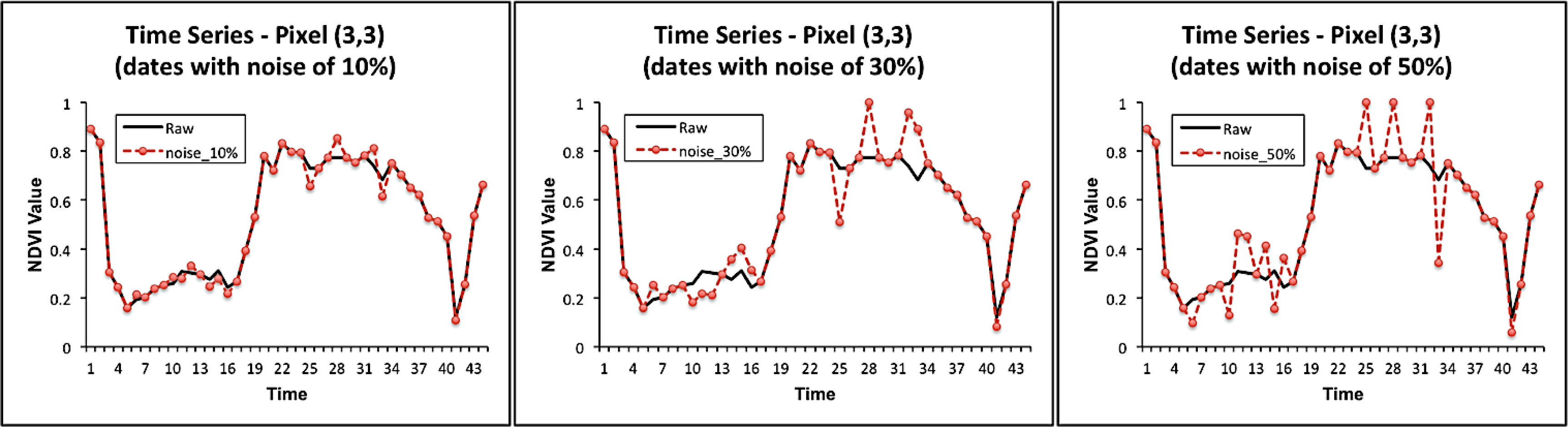
From the database, low quality time series were simulated by introducing noises according to [8,36]. This data simulation aims to assess the performance of the noise reduction process on the points considered as of low quality. The noise simulation process (or degradation) over time is constituted of random selection of dates where noise intensities will be applied onto original NDVI values. Three levels of noise were defined (10%, 30%, and 50%), and each level refers to the percentage randomly added or subtracted from the original NDVI value.

Figure 5 shows an example of degradation over time in which three levels of noise have been applied onto 12 dates of the time series of the pixel (3,3).

In addition to the noise simulation along the time series of a pixel, the database has also been degraded in relation to the number of pixels of low quality simulated in a same image. This degradation is performed with three intensities equivalent to 5%, 10%, and 20% of the image pixels.

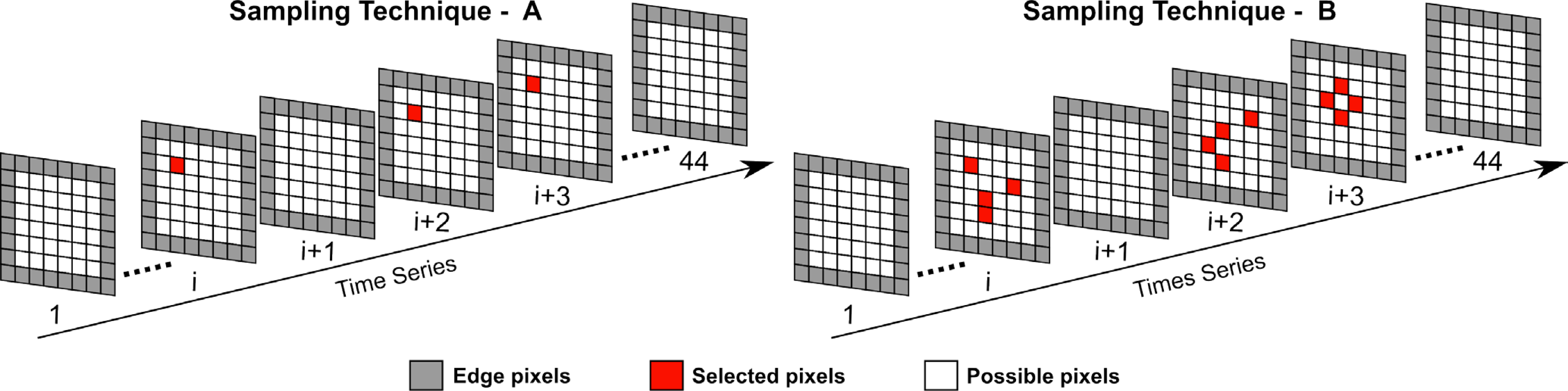
In order to evaluate the overall performance of the method proposed to reduce noise, two types of sampling that combine temporal and spatial degradation of data were performed. Additionally, the performance of the presented methodology will be compared to those results obtained by the filters 4253H twice; Savitzky–Golay and Mean Value Iteration. The sampling methods and performance evaluation methods are presented as follows.

5.1. Sampling Data for Analysis

The first step of the evaluation of methodology performance evaluation is the elaboration of sampling methods of pixels and dates to be analyzed within a same NDVI time series. This sampling aims to verify the spatial-temporal influence of noise simulation in time series on the results of the filtering techniques (mainly on the noise reduction method that uses spatial information in its analysis). Therefore, two types of noise sampling process were conducted: (A) sampling of the dates along the time series (temporal sampling); (B) sampling of the dates and pixels (spatial-temporal sampling).

The sampling method “A” consists of adding noise in a percentage of the dates of the temporal profile of a pixel of the study area. It is important to emphasize that the pixels in the borders of the images were not used in any sampling procedures. As a result, out of the 64 pixels (8 × 8 pixels matrix) in the study area, only 36 were considered apt for the sampling methods. Moreover, to reduce the effect of an absent data prior or posterior to the date to be analyzed, it has been established that only the intervals from the 4th to 41st date are apt for the sampling, as they comprise the time series (38 possible dates on a total of 44 dates). This study has defined that 30% of the dates that comprise the time series will be degraded; in sampling “A”, one pixel will be selected among the 36 pixels considered apt for the analysis; and it will be applied one noise level on 12 of the 38 possible dates.

The second sampling method simulates noise in time and space. This method uses the already described data interval of dates and pixels, but, for each selected date, noise is applied for more than one pixel of the image. Thus, 30% of the possible dates of the time series were selected and, for each selected date, a random percentage (5%, 10%, or 20%) of the pixels were chosen for simultaneous noise application. Figure 6 shows the two sampling methods.

5.2. Discrepancy Evaluation

This step aims to quantitatively evaluate the performance of the chosen filters for noise reduction. Therefore, for each pixel (R,C)i, where the noise has been added, a difference between the filtered and raw value was obtained to evaluate the fit in each simulation.

The importance of choosing the available statistical measures that best define the fit between the original value on the time series, and the result of the filtering process, was highlighted in [37]. The Root Mean Square Error (RMSE) is one of the traditional techniques used to measure the fit of the obtained results. However, Willmott and Matsuura [38] suggests the use of the Mean Absolute Error (MAE) to evaluate and compare the magnitudes of the discrepancies. This statistical measure (unlike RMSE) is an unambiguous measurement of the average error magnitude.

The techniques previously described to estimate the quality of the fit measure the differences between the correspondent raw and filtered data; thus, the higher the value of the dispersion the worse the result of the fit. However, these techniques have different evaluation emphases. MAE emphasizes the overall performance of the average, while RMSE stresses larger individual differences.

Nonetheless, the different scales in the time series may lead to inexpressive comparisons. Consequently, the Mean Absolute Percentage Error (MAPE) has been used here to compare the performance of the techniques. MAPE is expressed by:

$$\text{MAPE}=\frac{1}{\text{n}}\times \sum _{\text{i}=1}^{\text{n}}\left(\left|\frac{{\text{VI}}_{\text{i}\_\text{fit}}-{\text{VI}}_{\text{i}\_\text{obs}}}{{\text{VI}}_{\text{i}\_\text{obs}}}\right|\times 100\right)$$

(3)

where n is the number of evaluated points, VI_{i_fit} is the filtered value of the vegetation index, and VI_{i_obs} is the original value of the vegetation index in the time series.

Another statistical approach to evaluate the performances of the filtering techniques is the Akaike Information Criterion (AIC) [39,40]. It is calculated by using the following expression:

$$\text{AIC}=2\times \text{k}-2\times \text{log}(\text{L})$$

(4)

where k is the number of parameters of the model and L is the value of the likelihood. The lowest AIC values indicate the best performance of the model.

6. Results and Discussion

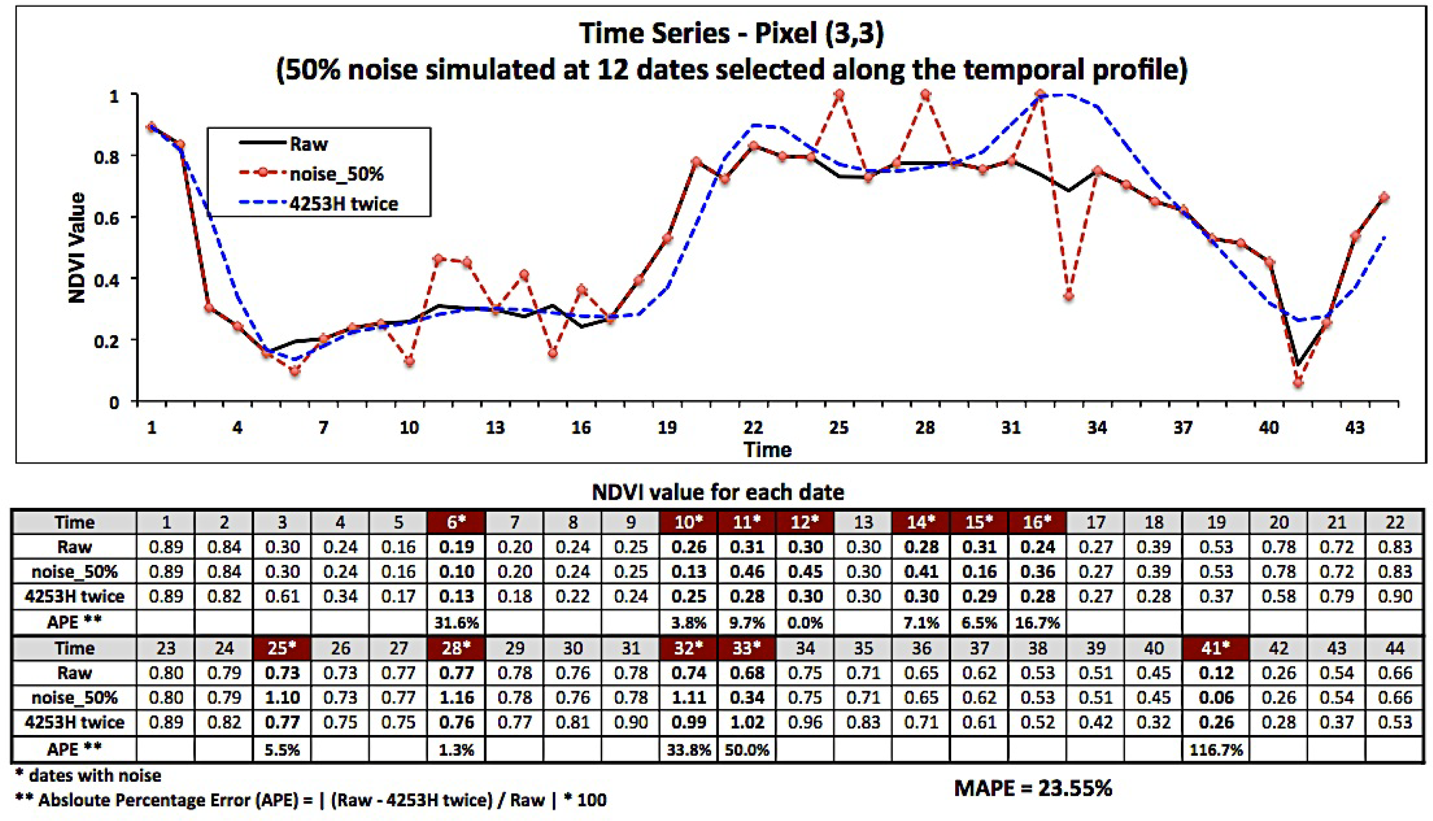
6.1. Temporal Sampling of the Noises

Sampling “A” proposes noise simulation along the time equal to 30% of the available dates in a NDVI temporal curve, i.e., for 12 dates of a pixel time series, three levels of noise (as shown in Figures 4 and 5) were applied. The method performance was analyzed for each level of noise, in addition to three other filtering techniques. Figure 7 illustrates the performance evaluation of the filter 4253H twice in a degraded time series with a noise equal to 50% by MAPE statistical measure.

The sampling procedures, including the techniques for noise reduction and the calculation of dispersion measurements, were repeated 1000 times for each level of noise.

Table 2. Descriptive analysis for the Mean Absolute Percentage Error (MAPE) values for the 1000 iterations done on sampling “A”.

Noise Level	Statistic Measures	Filters (% Value)
		4253H	MVI	SG	WR
10%	Min.	2.6	4.5	3.4	1.2
	Median	11.4	15.2	8.3	6.1
	Mean	14.2	16.8	9.2	6.9
	Max.	44.1	49.8	22.3	28.4
30%	Min.	4.3	3.9	9.5	1.2
	Median	13.7	16.9	16.4	6.1
	Mean	16.2	18.6	16.8	6.9
	Max.	49.7	53.7	32.3	28.4
50%	Min.	3.1	6.5	15.8	1.2
	Median	15.2	18.6	25.4	6.1
	Mean	17.3	20.2	25.7	6.9
	Max.	49.0	55.3	40.6	28.4

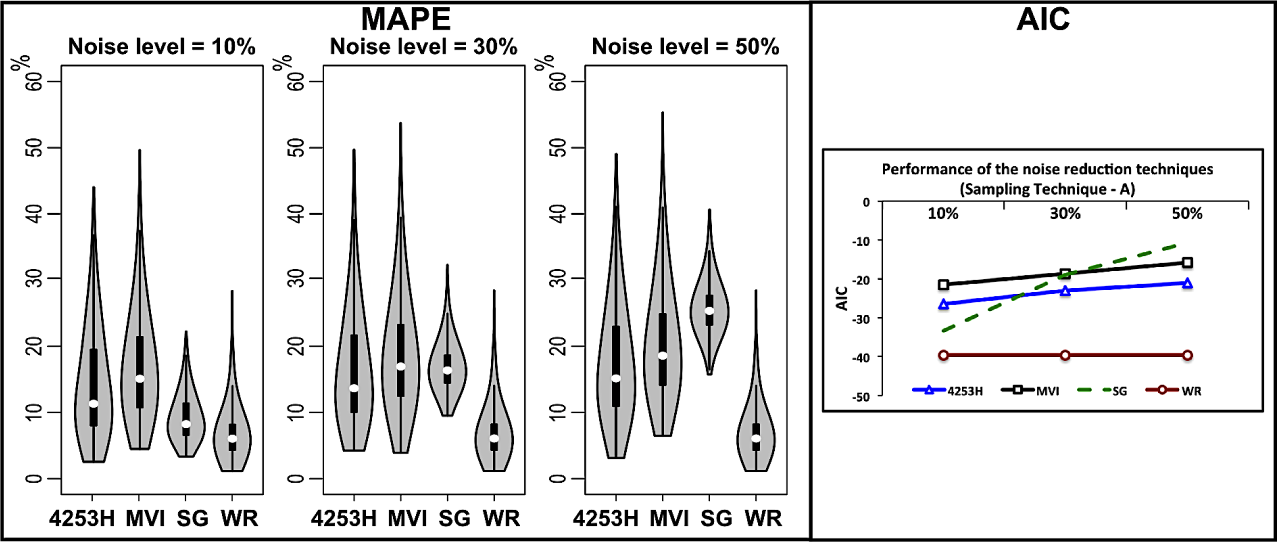
presents a descriptive analysis of the fit quality of the filtering techniques (4253H twice; Mean Value Iteration (MVI); Savitzky–Golay (SG); Window regression (WR)) for each level of noise analyzed. It can be observed that the lowest mean absolute percentage error values were obtained by the technique proposed in this work. Figure 8 illustrates the variation of the MAPE for each filtering technique and noise level applied on sampling “A”. According to [38], the lowest MAPE value refers to the best performance for the data set analyzed, i.e., the WR technique presented the best performance (lowest MAPE variation), amongst the techniques evaluated. The mean of the discrepant values for the WR filter was 7% lower, for all the three levels of noise applied, for both sampling methods.

The mean AIC value obtained for 1000 iterations is shown in Figure 8. It demonstrates a persistent performance of the WR technique for all the three noise levels. However, for the 4253H twice, MVI and SG filters, a decrease was observed in the performance by increasing noise intensity.

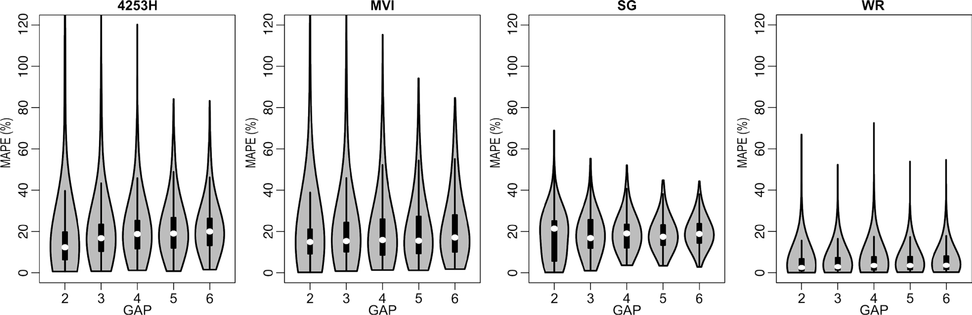
Regions such as the Amazon have intense cloud cover with periods longer than 30 days [41]. Thus, the temporal sampling was changed to simulate the influence of data gaps to estimate the new NDVI. The time series were changed by imposing data gaps (two to six sequential dates) and adding noise (equal to 30%). New NDVI values were estimated by each technique. The gap simulation results are shown in Figure 9, and again the WR technique presented the best accuracy. The mean MAPE values for the WR technique were the lowest among the other techniques, and did not exceed 7% for each gap level. Techniques 4253H, MVI, and SG, which use only the temporal information to estimate new values, showed variability in accuracies with different gap levels.

6.2. Spatial-Temporal Sampling of the Noises

A simulation of noise in time and in space is carried out in the sampling procedure “B”, where besides the 12 dates selected along the temporal profile, a number of pixels equal to 5%, 10%, and 20% were also sampled. This procedure was repeated 1000 times, for each simulation, on sampling “B”. It was also calculated the respective statistical measures, where the lowest MAPE and AIC values refer to the best fit for the original and filtered NDVI values.

Figure 10 presents the MAPE variation for each filtering technique noise level and simulated spatial degradation. The WR technique presented the best performance (lowest MAPE variation). On the other hand, 4253H twice, MVI and SG filters decreased the performance by increasing the noise level. In Sampling “B”, the WR technique provided discrepancy values similar to those obtained for sampling “A”, which presented mean MAPE values 7% lower for all the simulations performed.

The AIC values demonstrate that the WR technique provided better accuracy for the estimations of the new NDVI values for all simulations, in sampling “B” (Figure 11). Its behavior was constant irrespective of the number of pixels classified as of low quality in a scene. On the other hand, the other noise reduction techniques analyzed (4253H twice, MVI, and SG) presented lower accuracy as the level of noise applied increased. The SG filter presented the highest performance decrease.

The statistical measures that evaluated the performance of the filtering techniques presented the same behavior for both sampling methodologies, as shown in Figures 7 and 8. This is due to the fact that 4253H twice, MVI and SG filters only use temporal information of the curve. Thus, the presence of one or more degraded pixels, on the same date, do not affect their behaviors. However, the different sample sizes for each simulated spatial degradation led to changes in the dispersion of MAPE values (Figure 10).

Although the WR technique uses spatial information to estimate a value for a specific point, the degradation of 5%, 10%, or 20% of the pixels of the image did not affect the quality of the fit for this technique (Figure 10 and

Table 3. Mean of MAPE for 1000 iterations (Sampling “B”).

Spatial Degradation	Noise Level	Mean of MAPE (%)
		4253H	MVI	SG	WR
5%	10%	14.0	16.4	9.1	6.7
	30%	16.0	18.4	16.8	6.7
	50%	17.2	20.0	25.6	6.7
10%	10%	14.1	16.5	9.2	6.8
	30%	16.2	18.5	16.8	6.8
	50%	17.5	20.2	25.7	6.8
20%	10%	14.3	16.7	9.3	6.8
	30%	16.6	18.8	19.9	6.8
	50%	18.1	20.8	31.5	6.8

).

The individual AIC values are affected by sample size, so that large sample size decreases the AIC value. This is one of the factors that explains the different magnitudes of the AIC values in Figure 11. The dataset size for simulating the spatial degradation 20% is larger than other simulated degradations, which resulted in lower AIC values. However, the behavior of the curves prove that the higher the noise intensity applied, the worse the performance of 4253H twice, MVI, and SG filtering techniques. This behavior has been confirmed in all simulated spatial degradation. The noise level does not affect the WR technique, and this can be explained by the fact that a point classified as of low quality (or with noise) is not used to estimate the new value [42].

6.3. Performances of the Techniques

A non-parametric test was used to compare the performance of the noise reduction techniques analyzed in this study, through the assessment of the measurement positions among 1000 iterations. The MAPE values of one technique were compared and ordered according to the values obtained from the other three filters.

Table 4. Performances of the filtering techniques based on the Wilcoxon paired test of the MAPE values for the 1000 iterations.

Noise Level	Performance (1 is the best)	Sampling Technique A	Sampling Technique B (Spatial Degradation)
			5%	10%	20%
10%	1	WR	WR	WR	WR
	2	SG	SG	SG	SG
	3	4253H	4253H	4253H	4253H
	4	MVI	MVI	MVI	MVI
30%	1	WR	WR	WR	WR
	2	4253H	4253H	4253H	4253H
	3	SG	SG	SG	MVI
	4	MVI	MVI	MVI	SG
50%	1	WR	WR	WR	WR
	2	4253H	4253H	4253H	4253H
	3	MVI	MVI	MVI	MVI
	4	SG	SG	SG	SG

Note: All performances were significantly different (p value < 0.01).

presents the performance ranking of the filtering techniques based on the Wilcoxon paired test. It shows that the WR filter was statistically considered the most efficient for the three noise intensities simulated in this study, independently of the sampling technique. For the lowest noise level simulated, the SG filter presented the closest performance to the WR technique (Figures 7 and 8). However, as the noise level increased, the SG filter did not maintain its performance and moved from the second to the last position, in the performance ranking.

The simulated noises in time series were sorted into three intensities. The Window Regression (WR) and Savitzky–Golay filtering techniques provided the best fits for noise reduction at low intensity (10% noise), according to the MAPE and AIC values. For the 30% and 50% noise simulations, WR presented the best performance when compared to the other techniques. Noise intensity in the vegetation indices obviously affects the results obtained by the 4253H, MVI, and SG filtering techniques. On the other hand, it does not occur in the WR filtering technique, since the NDVI value of the pixel, along with the pixels considered as of low quality, are not used in the estimation of the new value of the pixel of interest. As expected, the techniques that use temporal information alone to estimate new values show decreased accuracy with amounts of data gap.

The 4253H twice, Mean Value Iteration and Savitzky–Golay techniques do not depend on the spatial information of the noise reduction procedure. However, different sample size in each simulated spatial degradation results in small changes in the mean MAPE values. Moreover, these techniques had their performances decreased by increased noise level, and SG filter presented the highest performance decrease rate (Figure 11).

The type of sampling did not affect the Window Regression (WR) technique performance, as demonstrated in Table 4. The performance of this technique by randomly selecting 30% of the dates along the spectral curve or by spatial degradation of the pixels up to 20% of the image/date was the best amongst the others. Although this technique maintains the performance for all noise levels or types of sampling, the quality of the fit between the filtered and original data is limited by the number of neighbors (both in space and in time) of guaranteed quality for a certain pixel to be analyzed. In general, the performance of the WR technique was satisfactory with until six consecutive degraded dates (gap); however, the selection criteria of spatial-temporal window lead this technique to be more negatively affected by gaps higher than 7 or by a greater number of pixels classified as of low quality at the same date.

The pixels on the edges of the image reduce the number of data available for analysis. The spatial window is represented by an analysis mask that is comprised by eight pixels neighboring the pixel of interest; but for the pixel at the corner of the image only three neighboring pixels will be available. Thus, for the pixels located at the edges of the image, the analysis will be possible with up to five neighboring pixels. However, this reduction in the number of neighboring pixels does not directly imply in decreased performance in the estimate of a new value, since a satisfactory adjustment can be obtained by the regression procedure.

7. Conclusions

The noise in NDVI time series caused by cloud contamination and atmospheric variability is considered a problem for the analyses of environmental changes, where the time series are used as input data in the models.

A new approach to estimate the pixels classified as of low quality has been proposed in this work, and the performance of this methodology was compared with other noise filtering techniques in NDVI time series. The performance of the Window Regression (WR) technique in the estimation of data with noise simulation in time alone was equal to its performance in noise simulation combining space and time. The combined analysis of the NDVI values in time-space, together with pixel quality information, proved to be a viable and promising alternative to estimate the pixels classified as of low quality noise in NDVI time series.

There are several methods for the reconstruction of NDVI time series, but only few of them use the information quality of the pixel in the noise reduction procedure or take into consideration the low quality data influence on the result. In [30], it is advised that the users of the MODIS products to inspect the science quality metadata, so that the product labeled with the lowest guarantee of quality should be used with caution. Hence we reaffirm the assertion of Musial et al. [37] that the choice for an approach of estimating lost values (or values of low quality) in time series depends on the underlying nature of the signal, the type and distribution of the data gaps, and the analyst expectation in obtaining data close to the existing data (low MAE) or requiring a representation of the general characteristics of the features of the time series.

The proposed method uses spatial-temporal analysis to estimate new NDVI value for a given pixel, and the analysis between neighboring pixels will be applied with caution in heterogeneous areas, or in more fragmented landscapes. Diverse land cover and land use spatial patterns result in spatial variability of NDVI values, and this variability can provide low correlation between neighboring pixels and, consequently, increased uncertainty of estimated values.

The results obtained in this research indicate that the method has good potential to reduce noise in MODIS NDVI time series data; however, more investigations are needed for noise reduction of NDVI time series from spatial-temporal analysis. The WR technique assumes that neighboring pixels with the same land use types are more correlated than pixels with different land use. Therefore, we suggest that future research works should include information about the land use types in the process of window spatial selection, so that pixels with different uses are excluded from the estimate of the new pixel value. The performance of this technique should be tested in regions with varying land use/land cover types, and compared with other noise reduction techniques. Lastly, continuous efforts are needed to develop and improve the modeling in time and space, in order to improve the representation of the dynamics of land cover and land use types.

References

- Justice, C.O.; Vermote, E.; Townshend, J.R.G.; Defries, R.; Roy, D.P.; Hall, D.K.; Salomonson, V.V; Privette, J.L.; Riggs, G.; Strahler, A.; et al. The Moderate Resolution Imaging Spectroradiometer (MODIS): Land remote sensing for global change research. IEEE Trans. Geosci. Remote Sens 1998, 36, 1228–1249. [Google Scholar]
- Pittman, K.; Hansen, M.C.; Becker-Reshef, I.; Potapov, P.V.; Justice, C.O. Estimating global cropland extent with multi-year MODIS data. Remote Sens 2010, 2, 1844–1863. [Google Scholar]
- Justice, C.O.; Townshend, J.R.G.; Vermote, E.F.; Masuoka, E.; Wolfe, R.E.; Saleous, N.; Roy, D.P.; Morisette, J.T. An overview of MODIS Land data processing and product status. Remote Sens. Environ 2002, 83, 3–15. [Google Scholar]
- Lasaponara, R. Estimating interannual variations in vegetated areas of Sardinia Island using SPOT/VEGETATION NDVI temporal series. IEEE Geosci. Remote Sens. Lett 2006, 3, 481–483. [Google Scholar]
- Bradley, B.A.; Jacob, R.W.; Hermance, J.F.; Mustard, J.F. A curve fitting procedure to derive inter-annual phenologies from time series of noisy satellite NDVI data. Remote Sens. Environ 2007, 106, 137–145. [Google Scholar]
- Sakamoto, T.; Yokozawa, M.; Toritani, H.; Shibayama, M.; Ishitsuka, N.; Ohno, H. A crop phenology detection method using time-series MODIS data. Remote Sens. Environ 2005, 96, 366–374. [Google Scholar]
- Ma, M.; Veroustraete, F. Reconstructing pathfinder AVHRR land NDVI time-series data for the Northwest of China. Adv. Space Res 2006, 37, 835–840. [Google Scholar]
- Hird, J.N.; McDermid, G.J. Noise reduction of NDVI time series: An empirical comparison of selected techniques. Remote Sens. Environ 2009, 113, 248–258. [Google Scholar]
- Holben, B.N. Characteristics of maximum-value composite images from temporal AVHRR data. Int. J. Remote Sens 1986, 7, 1417–1434. [Google Scholar]
- Atzberger, C.; Eilers, P.H.C. Evaluating the effectiveness of smoothing algorithms in the absence of ground reference measurements. Int. J. Remote Sens 2011, 32, 3689–3709. [Google Scholar]
- Velleman, P.F. Definition and comparison of robust nonlinear data smoothing algorithms. J. Am. Stat. Assoc 1980, 75, 609–615. [Google Scholar]
- Savitzky, A.; Golay, M.J.E. Smoothing and differentiation of data by simplified least squares procedures. Anal. Chem 1964, 36, 1627–1639. [Google Scholar]
- Chen, J.; Jönsson, P.; Tamura, M.; Gu, Z.; Matsushita, B.; Eklundh, L. A simple method for reconstructing a high-quality NDVI time-series data set based on the Savitzky–Golay filter. Remote Sens. Environ 2004, 91, 332–344. [Google Scholar]
- Swets, D.L.; Reed, B.C.; Rowland, J.D.; Marko, S.E. A. Weighted Least-Squares approach to Temporal NDVI Smoothing. In Proceedings of the ASPRS Annual Conference, Portland, OR, USA, 17–21 May 1999; pp. 526–536.
- Viovy, N.; Arino, O.; Belward, A.S. The Best Index Slope Extraction (BISE): A method for reducing noise in NDVI time-series. Int. J. Remote Sens 1992, 13, 1585–1590. [Google Scholar]
- Atzberger, C.; Eilers, P.H.C. A time series for monitoring vegetation activity and phenology at 10-daily time steps covering large parts of South America. Int. J. Digit. Earth 2011, 5, 365–386. [Google Scholar]
- Beck, P.S.A.; Atzberger, C.; Høgda, K.A.; Johansen, B.; Skidmore, A.K. Improved monitoring of vegetation dynamics at very high latitudes: A new method using MODIS NDVI. Remote Sens. Environ 2006, 100, 321–334. [Google Scholar]
- Zhang, X.; Friedl, M.A.; Schaaf, C.B.; Strahler, A.H.; Hodges, J.C.F.; Gao, F.; Reed, B.C.; Huete, A. Monitoring vegetation phenology using MODIS. Remote Sens. Environ 2003, 84, 471–475. [Google Scholar]
- Roerink, G.J.; Menenti, M.; Verhoef, W. Reconstructing cloudfree NDVI composites using Fourier analysis of time series. Int. J. Remote Sens 2000, 21, 1911–1917. [Google Scholar]
- Brooks, E.B.; Thomas, V.A.; Wynne, R.H.; Coulston, J.W. Fitting the multitemporal curve: A Fourier series approach to the missing data problem in remote sensing analysis. IEEE Trans. Geosci. Remote Sens 2012, 50, 3340–3353. [Google Scholar]
- Sakamoto, T.; Wardlow, B.D.; Gitelson, A.A.; Verma, S.B.; Suyker, A.E.; Arkebauer, T.J. A two-step filtering approach for detecting maize and soybean phenology with time-series MODIS data. Remote Sens. Environ 2010, 114, 2146–2159. [Google Scholar]
- Lu, X.; Liu, R.; Liu, J.; Liang, S. Removal of noise by wavelet method to generate high quality temporal data of terrestrial MODIS products. Photogramm. Eng. Remote Sens 2007, 73, 1129–1139. [Google Scholar]
- Chen, C.F.; Son, N.T.; Chen, C.R.; Chang, L.Y. Wavelet filtering of time-series moderate resolution imaging spectroradiometer data for rice crop mapping using support vector machines and maximum likelihood classifier. J. Appl. Remote Sens 2011. [Google Scholar] [CrossRef]
- Zhang, C.; Li, W.; Travis, D.J. Restoration of clouded pixels in multispectral remotely sensed imagery with cokriging. Int. J. Remote Sens 2009, 30, 2173–2195. [Google Scholar]
- Zhu, X.; Liu, D.; Chen, J. A new geostatistical approach for filling gaps in Landsat ETM+ SLC-off images. Remote Sens. Environ 2012, 124, 49–60. [Google Scholar]
- Pringle, M.J.; Schmidt, M.; Muir, J.S. Geostatistical interpolation of SLC-off Landsat ETM+ images. ISPRS J. Photogramm. Remote Sens 2009, 64, 654–664. [Google Scholar]
- Oliveira, J.C.; Epiphanio, J.C.N. Noise Reduction in MODIS NDVI Time Series Based on Spatial-Temporal Analysis. In Proceedings of the 2012 IEEE International Geoscience and Remote Sensing Symposium (IGARSS), Munich, Germany, 22–27 July 2012; pp. 2372–2375.
- Poggio, L.; Gimona, A.; Brown, I. Spatio-temporal MODIS EVI gap filling under cloud cover: An example in Scotland. ISPRS J. Photogramm. Remote Sens 2012, 72, 56–72. [Google Scholar]
- Cho, A.-R.; Suh, M.-S. Detection of contaminated pixels based on the short-term continuity of NDVI and correction using spatio-temporal continuity. Asia Pac. J. Atmos. Sci 2013, 49, 511–525. [Google Scholar]
- Roy, D.P.; Borak, J.S.; Devadiga, S.; Wolfe, R.E.; Zheng, M; Descloitres, J. The MODIS land product quality assessment approach. Remote Sens. Environ 2002, 83, 62–76. [Google Scholar]
- Huete, A.; Didan, K.; van Leeuwen, W.; Miura, T.; Glenn, E. MODIS Vegetation Indices. In Land Remote Sensing and Global Environmental Change: NASA’s Earth Observing System and the Science of ASTER and MODIS; Ramachandran, B., Justice, C.O., Abrams, M.J., Eds.; Springer: New York, NY, USA, 2011; pp. 579–602. [Google Scholar]
- Didan, K.; Huete, A. MODIS Vegetation Index Product Series Collection 5 Change Summary. MODIS Land Data Discipline Team,. 2006. Available online: http://landweb.nascom.nasa.gov/QA_WWW/forPage/MOD13_VI_C5_Changes_Document_06_28_06.pdf (accessed on 30 October 2013).
- Colditz, R.R.; Conrad, C.; Wehrmann, T.; Schmidt, M.; Dech, S. TiSeG: A flexible software tool for time-series generation of MODIS data utilizing the quality assessment science data set. IEEE Trans. Geosci. Remote Sens 2008, 46, 3296–3308. [Google Scholar]
- Kutner, M.H.; Neter, J.; Nachtsheim, C.J. Applied Linear Regression Models, 4th ed.; McGraw-Hill Higher Education: Boston, MA, USA, 2004; p. 701. [Google Scholar]
- Wardlow, B.; Egbert, S.; Kastens, J. Analysis of time-series MODIS 250 m vegetation index data for crop classification in the U.S. Central Great Plains. Remote Sens. Environ 2007, 108, 290–310. [Google Scholar]
- Adami, M. Estimativa da Data de Plantio da soja por Meio de Séries Temporais de Imagens MODIS. Ph.D. Dissertation, INPE, São José dos Campos, SP, Brazil. 2010. [Google Scholar]
- Musial, J.P.; Verstraete, M.M.; Gobron, N. Comparing the effectiveness of recent algorithms to fill and smooth incomplete and noisy time series. Atmos. Chem. Phys. Discuss 2011, 11, 14259–14308. [Google Scholar]
- Willmott, C.J.; Matsuura, K. Advantages of the mean absolute error (MAE) over the root mean square error (RMSE) in assessing average model performance. Clim. Res 2005, 30, 79–82. [Google Scholar]
- Akaike, H. Information Theory and an Extension of the Maximum Likelihood Principle. In Proceedings of the Second International Symposium on Information Theory, Akaddemiai Kiado, Budapest, Hungary, 2–8 September, 1973; pp. 267–281.
- Atkinson, P.M.; Jeganathan, C.; Dash, J.; Atzberger, C. Inter-comparison of four models for smoothing satellite sensor time-series data to estimate vegetation phenology. Remote Sens. Environ 2012, 123, 400–417. [Google Scholar]
- Asner, G.P.; Alencar, A. Drought impacts on the Amazon forest: The remote sensing perspective. New Phytol 2010, 187. [Google Scholar]
- Oliveira, J.C.; Epiphanio, J.C.N.; Renno, C.D. The Use of Spatial-Temporal Analysis for Noise Reduction in MODIS NDVI Time Series Data. In Proceedings of the 10th International Symposium on Spatial Accuracy Assessment in Natural Resources and Environmental Sciences (Accuracy 2012), Florianópolis, SC, Brazil, , 10–13 July 2012.
© 2014 by the authors; licensee MDPI, Basel, Switzerland This article is an open access article distributed under the terms and conditions of the Creative Commons Attribution license (http://creativecommons.org/licenses/by/3.0/).