Article

On the Response of European Vegetation Phenology to Hydroclimatic Anomalies

1
Institute for Environment and Sustainability, DG Joint Research Centre, European Commission, Ispra 21027, Italy
2
Biogeochemical Integration Department, Max Planck Institute for Biogeochemistry, Jena 07745, Germany
*
Author to whom correspondence should be addressed.
Remote Sens. 2014, 6(4), 3143-3169; https://doi.org/10.3390/rs6043143
Submission received: 20 January 2014 / Revised: 21 March 2014 / Accepted: 31 March 2014 / Published: 9 April 2014

Abstract

:
Climate change is expected to alter vegetation and carbon cycle processes, with implications for ecosystems. Notably, understanding the sensitivity of vegetation to the anomalies of precipitation and temperature over different land cover classes and the corresponding temporal response is essential for improved climate prediction. In this paper, we analyze vegetation response to hydroclimatic forcings using the Fraction of Absorbed Photosynthetically Active Radiation (FAPAR) derived from SeaWiFS (Sea-viewing Wide Field-of-view Sensor) (1998–2002) and (Medium Resolution Imaging Spectrometer) (2003–2011) satellite sensors at ∼1-km resolution. Based on land cover and pixel-wise analysis, we quantify the extent of the dependence of the FAPAR and, ultimately, the phenology on the anomalies of precipitation and temperature over Europe. Statistical tests are performed to establish where this correlation may be regarded as statistically significant. Furthermore, we assess a statistical link between the climate variables and a set of phenological metrics defined from FAPAR measurement. Variation in the phenological response to the unusual values of precipitation and temperature can be interpreted as the result of the balanced opposite effects of water and temperature on vegetation processes. Results suggest very different responses for different land cover classes and seasons. Correlation analysis also indicates that European phenology may be quite sensitive to perturbations in precipitation and temperature regimes, such as those induced by climate change.

1. Introduction

During the last decade, there has been an increasing interest in understanding the interactions between land cover (particularly vegetation) and climate, in order to assess the impacts of climate change on the carbon cycle [16]. Climate change can be expected to have an important impact on the water and energy cycles (in both phase and amplitude), thereby significantly affecting vegetation [7]. Conversely, vegetation plays a role in impacting the carbon cycle, thus completing a “feedback loop” with the climate [811]. For this reason, the response of vegetation dynamics, for different land cover types, to precipitation and temperature anomalies is a subject of current climate research [1219], aimed at understanding (and predicting) how the biosphere interacts with the atmosphere through the carbon, water and energy cycles [2023].
Work by Los et al. [24] and, more recently, Wang et al. [25] and Beer et al. [26] led to a better understanding of vegetation response to climate signals. Forzieri et al. [27] explored the correlation structures of vegetation dynamics and climate over the southwestern region of North America. Other studies have focused on the vegetation response to events that deviate from the expected patterns by two or more standard deviations (i.e., extreme climate events): Ciais et al. [28] and Gobron et al. [29], for example, analyzed the Europe-wide reduction in primary productivity caused by the heat wave and drought of 2003. Furthermore, Diffenbaugh [30] quantified the vegetation response of extreme climate regimes in the western USA, while Lorenz et al. [31] found an important feedback between vegetation phenology and climate extremes over Europe. Reichstein et al. [32] addressed the implication of climate extremes on the global terrestrial carbon budget.
Other than local studies, which often focus on extreme climate events only, the sensitivity of vegetation to climate variability has not yet been fully analyzed and understood at a European scale. Europe is a region of particular interest, as it is likely to experience changes in the annual distribution of hydroclimatic variables, such as precipitation and temperature [33]. The availability of information on the spatio-temporal patterns of the response of vegetation phenology to precipitation and temperature anomalies is extremely important. The higher the spatial resolution of the information, the more reliable is the assessment of the phenology response to anomalous events, for different seasons and/or land cover types.
This study characterizes the impacts of anomalies in hydroclimatic variables, such as precipitation and temperature, on land vegetation across Europe (defined by geographic coordinates 33°N–72°N; 32°W–55°E). The Fraction of Absorbed Photosynthetically Active Radiation (FAPAR), a satellite-derived indicator of vegetation phenology, is used together with a spatially-distributed dataset of precipitation and temperature values (see the Materials and Methods section) as the basis on which to quantify the impacts of hydroclimatic anomalies on vegetation, for the period of 1998–2011, at a spatial resolution of 1 km.
Specifically, the objectives of the study are: (1) to identify statistically significant spatial patterns of correlation between anomalies of FAPAR, precipitation and temperature; (2) to analyze the corresponding temporal response patterns; and (3) to examine the dependence of these patterns on land cover, determining whether different land cover types amplify or attenuate the effect of hydroclimatic forcing factors on vegetation dynamics.
Considering both its wide geographic scope and high spatial resolution, the study represents an important step towards the assessment of large-scale climate change impacts on vegetation.

2. Materials and Methods

In this study, the impact of hydroclimatic variables on vegetation over Europe is considered, based on an analysis of precipitation, temperature and FAPAR anomalies during the period of 1998–2011, at monthly and annual time steps. As outlined in more detail below, anomalies translate hydroclimatic variables into simple indicators that can be used both for analyzing correlations and for relaying information to a wider audience in a clear form. In order to assess the differential responsiveness of land cover, the study area used corresponds to the region for which the CORINE (Co-ORdination of INformation on the Environment) Land Cover 2006 database [34,35] is available.

2.1. FAPAR Data and Computation of Anomalies

FAPAR is a biophysical parameter that refers to the state and photosynthetic activity of the plant canopy [36]. It is directly correlated with the primary productivity of vegetation and is recognized as one of the 50 essential climate variables, defined by the UN’s Global Climate Observing System (GCOS), that characterize the Earth’s climate [37,38]. The systematic observation of FAPAR is suitable for monitoring the strength and location of terrestrial carbon pools and fluxes [39,40]. FAPAR datasets are used, for example, as part of the Carbon Cycle Data Assimilation System (CCDAS) project, in order to improve terrestrial carbon simulations [4143] or to estimate global land evapotranspiration [44]. The contribution of FAPAR in the monitoring of harvests is summarized by Rembold et al. [45], while its use for sugarcane yield forecasting and monitoring over São Paulo, Brazil, is described by Duveiller et al. [46].
The FAPAR time series used in this study is derived from near-daily observations in the red, near-infrared and blue spectral bands, captured by National Aeronautics and Space Administration’s NASA-SeaWiFS (Sea-viewing Wide Field-of-view Sensor) and European Space Agency’s ESA-MERIS (Medium Resolution Imaging Spectrometer) satellite sensors. The SeaWiFS data were for the period of 1998–2004, and the MERIS data for 2002–2011 [47,48]. The nominal spatial resolutions were, respectively, 1.5 km and 1.2 km.
A compositing algorithm [49,50] is applied to the SeaWIFS and MERIS products to generate decadal estimates (i.e., sequences of nominally 10 consecutive days, starting from the first day of the month, where the last period may contain from 8 to 11 days) from the original (quasi-daily) values. Specifically, the actual FAPAR value, which is closest to the arithmetic mean for the period, is chosen as the most representative. In order to build a spatially consistent time series, the FAPAR products are re-sampled to grids of ∼1 km (i.e., longitudinal sampling interval = 0.016°, latitudinal sampling interval = 0.011°) using nearest-neighbor interpolation.
To obtain a consistent FAPAR measurement throughout the entire time period, the corresponding observations from both sensors have been merged using a harmonization procedure, whereby the products are: (a) corrected to remove remaining noise contamination; (b) gap-filled; and (c) bias-corrected using two common years of observations (for further details, see [51]).
Due to the seasonal behavior of both the mean and standard deviation FAPAR (not shown here), the dataset is transformed to become stationary up to the 2nd order. Anomalies of FAPAR (hereafter, called “AFAPAR”) are computed using the Z-scores with a reference period of 14 years with Equation (1).
A t = X t X ¯ t σ t
where At is the resulting anomalies, Xt is the decadal (i.e., 10-day period) FAPAR, t is the mean over the period of reference for each decade, σt is the standard deviation for each decade and t is the decade. To generate the monthly AFAPAR, decadal FAPAR time series are averaged.

2.2. Anomalies of Rainfall and Temperature

The data for precipitation and mean surface temperature are collected from the daily gridded datasets (E-OBS) for surface climate variables [52] available via the European Commission’s 6th Framework Programme project, ENSEMBLES [53], with a spatial resolution of 0.25°.
The precipitation anomalies are calculated at monthly time scales through the Standardized Precipitation Index (SPI) [54] and at annual time scales through the Z-scores. SPI, estimated by transforming the observed rainfall distribution into a standardized normal distribution, is one of the most widely used indices within drought and flood monitoring systems [55,56]. Positive values indicate wet conditions and negative values dry conditions, with the more extreme values indicating the more severe anomalies.
Since different water resources (e.g., soil moisture, streamflow and groundwater) respond to precipitation deficits at different temporal scales, SPI may be calculated for different time frames (e.g., 1, 3, 6, 12 months). An exploratory analysis has been performed to determine the appropriate time frame for computing SPI (not shown here). Results indicate that SPI generally has the strongest correlation with vegetation response over Europe at time scales of three months. This observation is consistent with the concept of lagged vegetation response to rainfall anomalies [16,57]. Thus, only the 3-month SPI (hereafter called “SPI-3”) is used for subsequent analyses.
Annual anomalies of rainfall are calculated using the Z-scores, computing first the departures from the average annual precipitation and then dividing by the standard deviation. To avoid considering processes that are not strongly correlated with phenology, winter precipitation (i.e., December, January, February) is excluded from the computation of the annual anomaly.
Anomalies of temperature (hereafter, called “AT”) are calculated for the period of 1998–2011 through the Z-scores both at the monthly and annual time scale. Again, winter temperature (i.e., December, January, February) is excluded from the computation of the annual anomaly.
In order to build coherent and consistent time-series, all of hydroclimatic dataset is re-sampled to the spatial resolution of the FAPAR dataset of ∼1 km (i.e., longitudinal sampling interval = 0.016°, latitudinal sampling interval = 0.011°).

2.3. Phenology Metrics

Following the method proposed in Jung et al. [40] and updated by Ceccherini et al. [58], four phenology indicators are calculated for each calendar year from the 10-day FAPAR time series: mean FAPAR, maximum FAPAR, growing season length (GSL) and cumulative FAPAR of the growing season (CGS).
The growing season length (GSL) is calculated by assuming that the annual FAPAR record is shaped like a semi-ellipse. The corresponding area is calculated as the sum of FAPAR values for the year, following the subtraction of a “background” value. The latter is calculated as 20% of the maximum value of the FAPAR time series for each pixel during one calendar year: FAPAR generally may not decrease to zero, because of the vegetated background below the canopy; hence, this value is typical for non-growing season conditions. Given the area and the major axis of the ellipse (i.e., annual maximum FAPAR minus the “background”), the minor axis of the ellipse (i.e., GSL) can be retrieved.
Finally, the cumulative FAPAR of the growing season of a calendar year (CGS) is estimated as the sum of FAPAR values of a year from the start to the end of the growing season. For further details on the methodology, see [58]. Note that Jung et al. [40] used a background equal to the 10th percentile of the annual FAPAR time series. The value of 20% of the maximum value of the FAPAR is used here, based on the result of a sensitivity analysis for testing the effectiveness of the threshold values.
Phenological metrics are important because of the effect of phenology on the climate-biosphere interaction, through the regulation of carbon, water and energy fluxes [20,23,59]. Maximum FAPAR is associated with the peak of photosynthetic activity during the growing season, whereas CGS is a useful indicator of net primary productivity [40,60]. Figure 1 depicts the spatial patterns of the phenology indicators corresponding to climatological averages for the period of 1998–2011.
Anomalies of phenology metrics are calculated through the Z-scores at the annual time scale.

2.4. Land Cover

Information on land cover is taken from CORINE Land Cover ([34,35], version 16, April 2012) (hereafter, CLC2006), available from the European Environment Agency ( http://www.eea.europa.eu/). The CLC2006 map discriminates 44 land cover classes at a spatial resolution of 100 m, with a high level of accuracy (greater than 85%, according to EEA [35]). The original dataset is resampled to the same spatial resolution of the FAPAR dataset. In this process, the CLC2006 class with the highest occurrence is assigned to each pixel. Only the five major vegetated European land cover classes, namely “broadleaved forest”, “coniferous forests”, “mixed forest”, “arable land” and “permanent crops”, are analyzed. The class “heterogeneous agricultural areas” is excluded. Arable land includes many land cover types, such as non-irrigated and permanent irrigated arable land and rice fields, while permanent crops include vineyards, olive groves and fruit trees and berry plantations. In Figure 2, the five broad land cover categories from CLC2006 are shown. Finally, these five land cover classes are merged into two broad classes: “forest” and “agriculture”.

2.5. Correlation Analysis

Since anomalies in the water, energy and carbon cycles interact with each other, the impact of hydroclimatic forcings on the phenological cycle can be amplified or dampened. In order to understand the linkages between the components of the system, various correlation analysis techniques are used to quantify the ecosystem response to precipitation and temperature anomalies.
Firstly, the linkage between precipitation/temperature and FAPAR is analyzed at the pixel level and at a monthly time scale, using cross-correlation at a significance level of 95% (p = 0.05). Cross-correlation is a measure of the similarity of two signals as a function of the time-lag applied to one of them. To consider the characteristic time-lag between climate forcings and vegetation response, the temperature and the rainfall time series are shifted against the FAPAR time series before correlation. The time-lagged correlation analysis is performed with four monthly lags (i.e., lag 0, lag −1, lag −2, lag −3); the anomalies of FAPAR of one month are correlated with the anomalies of the precipitation/temperature of the same month (lag 0), of the previous month (lag −1), and so on. Lags longer than 3 months are excluded.
Secondly, the correlation between the yearly anomalies of the phenology metrics and hydroclimatic variables is analyzed by means of the Pearson’s correlation at the same significance level (95%). Pearson’s correlation is a measure of the linear correlation between two signals indicating how they vary jointly.
Finally, the rank correlation, a measure of the strength of the associations between two variables, is calculated using the Spearman’s rank correlation test [61]. The test is performed between monthly anomalies of FAPAR, precipitation and temperature, for the 12 months of the year, at the pixel level. Anomalies of phenology metrics are excluded from this analysis, and no time-lag between climate and vegetation is considered. The Spearman’s rank correlation allows one to investigate the statistical dependence of data without assuming any particular joint probability distribution of the two variables. Furthermore, it is less prone to the influence of outliers in the dataset, as it is non-parametric. The sign of the Spearman correlation indicates the direction of association between anomalies of FAPAR and the anomalies of temperature and rainfall. If the value of AFAPAR increases (or decreases) when AT (anomalies of temperature)/SPI-3 increases (or decreases), the Spearman correlation coefficient is positive. The Spearman correlation increases in magnitude as the two variables approach a perfect monotonical relationship. FAPAR/hydroclimatic correlation results are both presented in a spatially explicit way and spatially averaged per land cover category.

3. Results

The need to characterize the spatial linkages and temporal dynamics of seasonal hydroclimatic and terrestrial biophysical variables over Europe is highlighted in Figure 3. Monthly anomalies of temperature, precipitation and FAPAR are shown for two contrasting wet and dry periods (August 2002, and August 2003, respectively) over the western part of Europe [62,63]. Anomalies of temperature and precipitation are consistently shown to have an important influence on the phenological cycle, but separately do not explain all the FAPAR variability. Thus, both variables must be analyzed. Figure 3 also shows that the great spatial variability of climate anomalies, underlining the importance of using remote sensing datasets.

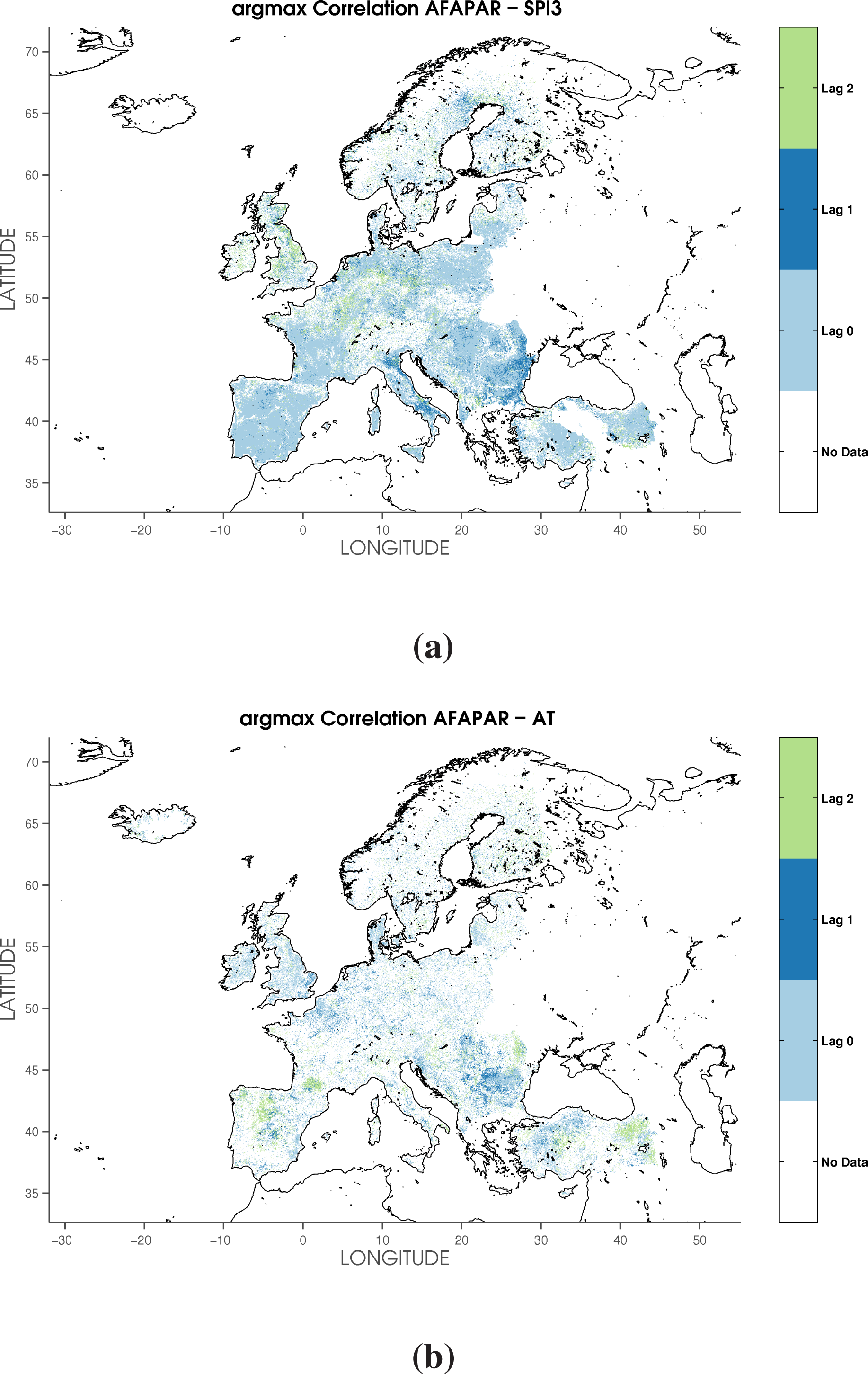
3.1. Cross-Correlation between FAPAR and Hydroclimatic Anomalies

Figure 4 shows the spatial patterns for the correlation coefficient (ρ) between anomalies of FAPAR and anomalies of precipitation/temperature. Each point in the maps represents the maximum absolute value of the cross-correlation over the same month or the previous ones (up to lag 3). Since signals may show a negative correlation, we calculate the maximum absolute value of the cross-correlation coefficient during the three-month period, to highlight the vegetation responses to rainfall/temperature perturbations that persist for up to three months. Figure 4 indicates very distinct regional areas that present a positive (blue) or negative (red) correlation. Only significant correlations are shown: the hypothesis test is rejected with a significance level of 95% (p = 0.05).
The correlation values for SPI-3 and AT, shown respectively in Figure 4a,b, generally do not follow a latitudinal gradient. A first examination shows that FAPAR anomalies have a significant correlation with SPI-3 and AT for 43.60% and 19.14% of the study area. SPI-3 is the more influential variable for phenological variability, with a generally positive correlation. Figure 4a indicates that 38.77% of the study area has a positive correlation, while 4.83% has a negative correlation. The high degree of correlation between AFAPAR and SPI-3 indicates that the latter variable captures the ecologically significant accumulated precipitation surplus or deficit, in accordance with the conclusion of Rossi et al. [64] and Sepulcre-Canto et al. [16]. Results also indicate important latitudinal responses: temperature anomalies are negatively correlated to FAPAR anomalies at a lower latitude and positively correlated in the northern regions. Figure 4b suggests a smaller sensitivity of FAPAR to temperature than to precipitation. Areas presenting a positive correlation (10.44%) are larger than those presenting negative ones (8.70%).
By using the CLC2006 database, we are able to extend this analysis to examine the percentage of each land cover class where the correlation is significant (Table 1). Table 1 also shows the spatial-average of correlation coefficients (i.e., ρ) for positive and negative correlations separately. In Table 1, the first two columns show the percentage of land cover classes where the correlation for rainfall (SPI-3) and temperature (AT) anomalies is significant at the 95% level. The last four columns show the spatial-average of the correlation coefficient—ρ—for SPI-3 and AT for positive (pos.) and negative (neg.) values separately.
Positive and negative correlations represent very different ecosystem responses to climate anomalies, and they are associated with very different mechanisms. While a positive value of the correlation points out that hydroclimatic anomalies may support the photosynthetic activity of vegetation, a negative correlation may indicate a negative feedback. Regarding the anomalies of precipitation, ρ is always higher for positive rather than for negative correlation, in accordance with the results in Figure 4. For anomalies of temperature over forest classes, ρ is higher for negative than for positive correlation, while the opposite applies for agricultural classes, indicating a differential responsiveness of land cover. FAPAR for arable land and permanent crop shows the highest correlation with precipitation. For broadleaved forest, the correlation coefficient with both precipitation and temperature is higher than for coniferous and mixed forest. Generally, ρ is higher for precipitation than for temperature for both positive and negative correlations. The spatial standard deviation (not shown here) ranges from 0.01 of temperature to 0.02 of precipitation.
Figure 5a,b shows which lag gives the maximum of the correlation for each pixel for both SPI-3 and AT, respectively, while Table 2 reports the distribution of the time-lag for the five main CLC2006 land cover categories. The analysis performed with the three-month lag (i.e., lag −3) shows no significant correlation for either SPI-3 or AT. Analysis of the two-month lag indicates a steep fall-off in the spatial extent of the correlation for all the land cover classes, for both SPI-3 and AT.
Regarding SPI-3, the maximum correlation is almost instantaneous (i.e., within one month), even if SPI-3 continues influencing AFAPAR also after 1 month. Figure 5a indicates a strong effect also with a lag equal to 1 and 2. Agriculture (i.e., arable land and permanent crop) is the land use type with the greatest response to rainfall, which persists up to two months. Spatial responses in forests are also significant, but less persistent, indicating that these land cover categories are less dependent on water availability than agricultural classes. Delayed reaction patterns to precipitation have been reported for estuarine areas (e.g., Po, Danube). This shows that anomalous vegetation conditions may be more related to the precipitation accumulated in the basin over a period of time than to the instantaneous and local one. As with SPI-3, the most noticeable result for AT is the predominant decrease of correlation from lag 0 to lag 1 across Europe, but spatial patterns generally differ from SPI-3. Temperature perturbations propagate rapidly (0-month lag), with a significant low-persistence (2-month lag) for the FAPAR response. Temperature effects on coniferous and mixed forest are the most persistent (up to two months).

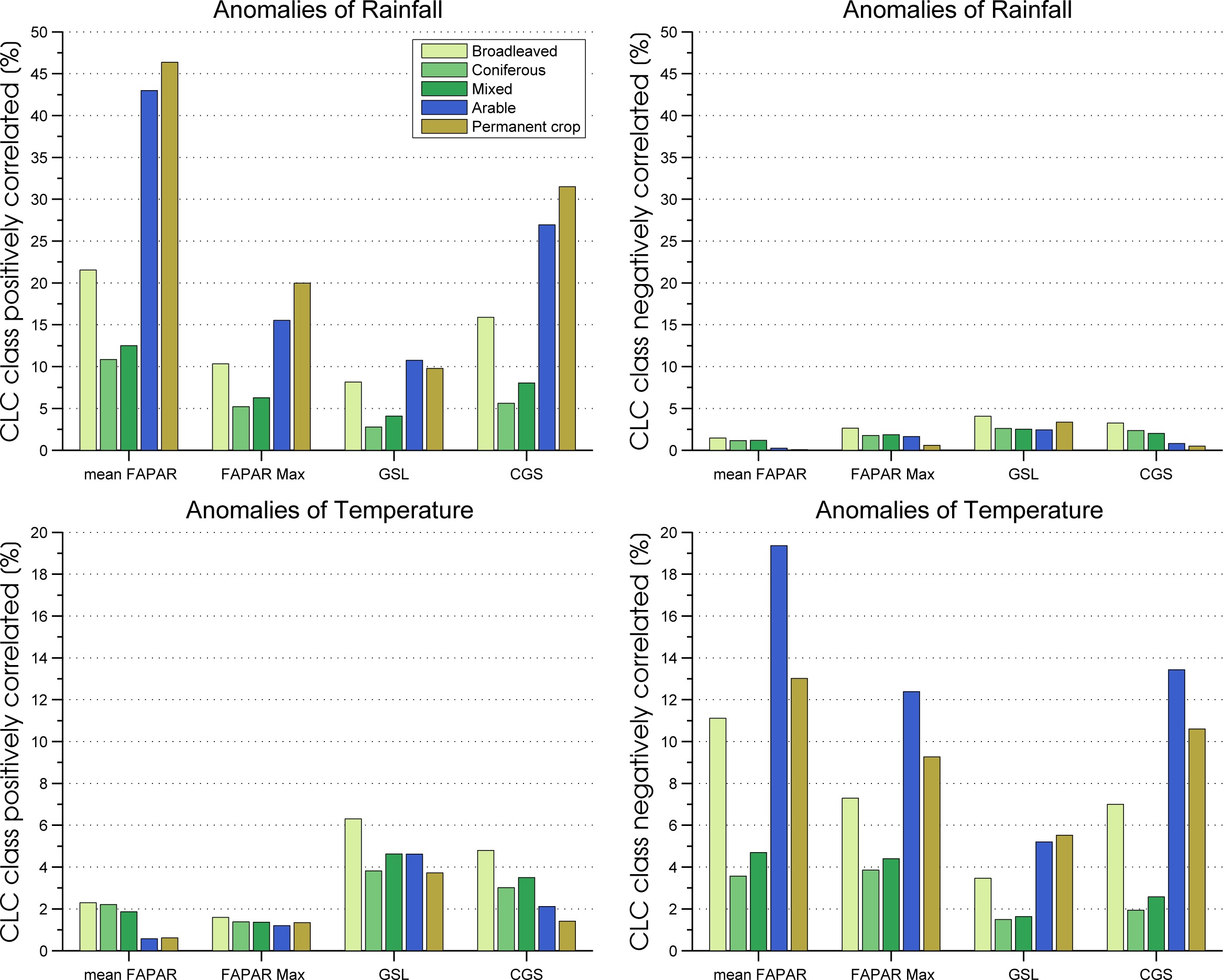
3.2. Correlation between Phenology Metrics and Hydroclimatic Anomalies

Figure 6 summarizes the sensitivity of vegetation metrics to perturbations in precipitation and temperature regimes.
Since the anomalies have been calculated with only 14 values (i.e., annual values for the period of 1998–2011), the annual rainfall and temperature anomalies used correspond with the time scale of vegetation metrics. For temperature, the areas presenting negative correlation are larger than those presenting positive correlation, whereas the opposite behavior is seen for precipitation.
Figure 6 indicates the spatial effect of the anomalies of precipitation and temperature on the main phenology metrics. Results generally reflect a lower sensitivity of the vegetation metrics to temperature than to precipitation. For rainfall, mean FAPAR shows the highest percentage of covered area with a positive correlation. In contrast, a more moderate spatial extent of correlation is obtained for temperature than for precipitation. Furthermore, AT generally shows a high negative correlation. FAPAR max and CGS have lower correlations with rainfall or temperature than mean FAPAR, although still being highly significant (p = 0.05). These results indicate that mean FAPAR is the most sensitive metric, while GSL is the least sensitive. FAPAR max presents some patterns similar to mean FAPAR, with less area involved. The geographical distribution of Pearson’s correlation coefficient between AT and CGS suggests a negative correlation over the Carpathian region (i.e., 45°N, 20°E).
Maps in Figure 6 are complemented by spatial statistics for each phenology metrics summarized in Table 3, which details the percentage of the study area where the correlation between the anomalies of phenology metrics and the hydroclimatic variables are significant.
As is evident in Figure 6, phenology metrics reflect a smaller sensitivity to temperature than to precipitation anomalies. The spatial extent of positive correlation between phenology metrics and SPI-3 ranges from 7.3% of GSL and 26.8% of mean FAPAR, whereas areas of negative correlation are always below 3%. Regarding temperature, phenology metrics exhibit the opposite behavior: mean FAPAR, maximum FAPAR and CGS show a predominance of negative correlation, and vice versa for GSL. The dominance of positive (for precipitation) and negative (for temperature) spatial patterns suggests corresponding positive and negative feedback between precipitation and temperature anomalies and phenology metrics. The spatial extent of the sum of positive and negative correlation with temperature is generally around 8%–13% and 10%–27% for SPI-3.
Figure 7 presents histograms showing the percentage of the study area where the correlation is significant for each land cover class, shown separately for positive and negative correlations. Regarding the positively correlated rainfall anomaly, forest classes show a smaller area than agricultural ones. Mean FAPAR exhibits the highest spatial extent of correlation and GSL the lowest. A common feature obtained for all phenology metrics except GSL is that permanent crop exhibits a greater area than arable land. A moderate spatial extent of correlation is obtained for negative precipitation anomalies: generally, the spatial extent decreases by roughly a factor of four between positive and negative correlation. Regarding both positively and negatively correlated temperature anomalies, the spatial extent of correlations ranges from 2% to 20% of CLC classes, far less than the positive rainfall correlation. Generally, vegetation metrics present higher spatial correlation with negative than with positive temperature anomalies, with the exception of the forest classes of GSL. Among the forest classes, broadleaved forest shows the highest spatial extent of correlation, whereas coniferous forest appears less sensitive, for both positive and negative correlation and for both rainfall and temperature anomalies.

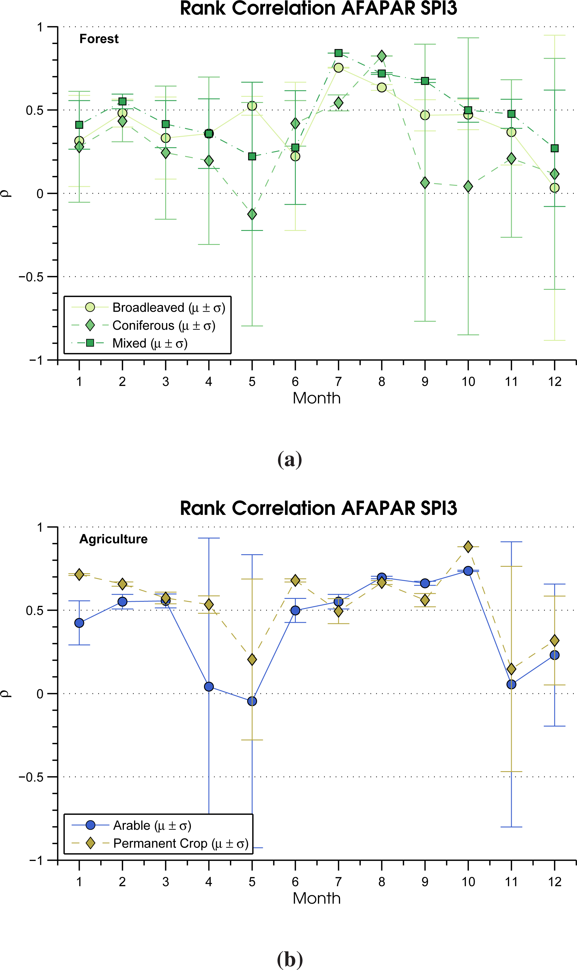
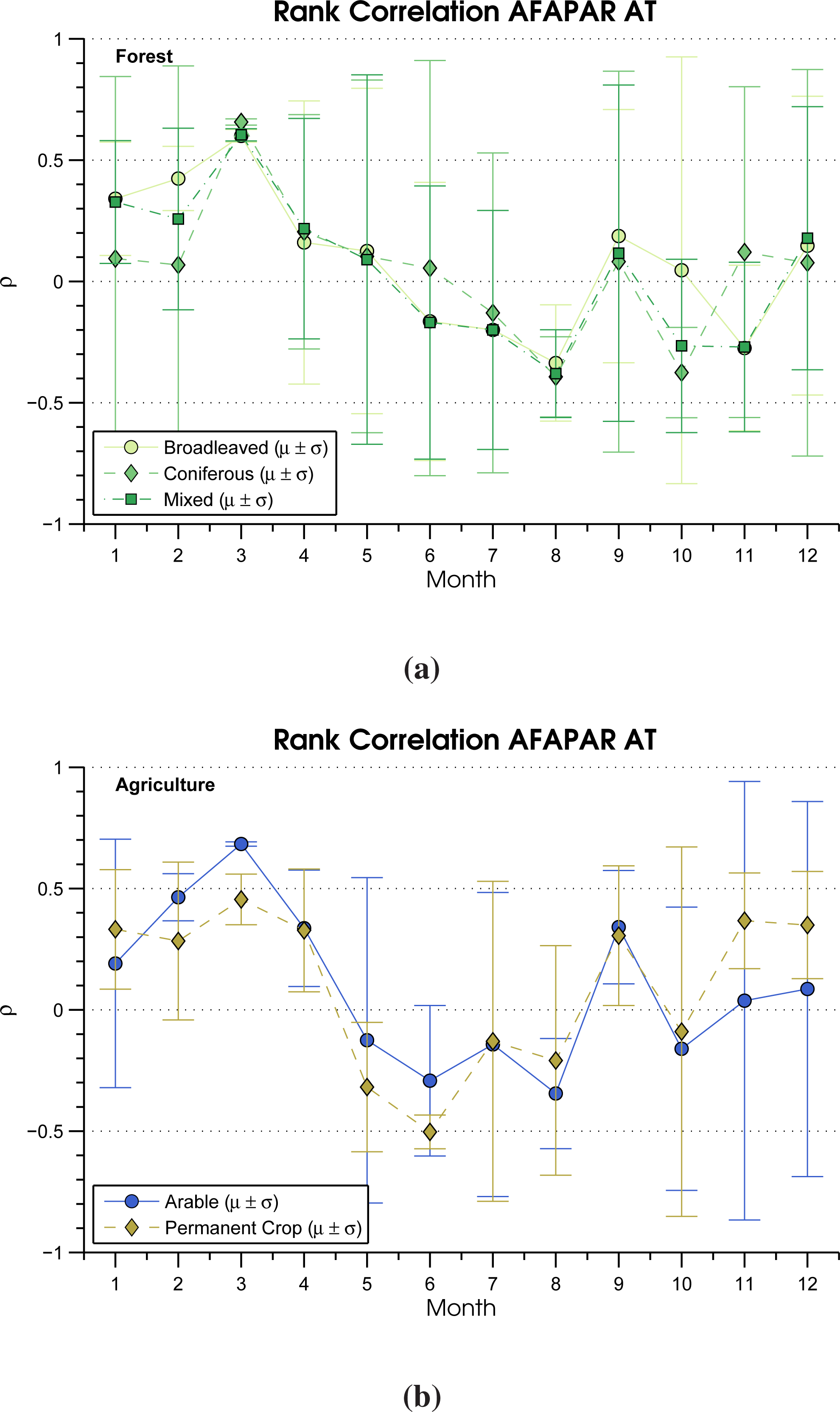
3.3. Rank Correlation

Figures 8 and 9 present the spatial-averaged monthly rank correlation (i.e., a measure of monotone association) and the corresponding spatial-averaged standard deviation between anomalies of FAPAR and SPI-3/AT for different CLC2006 land cover types. The smaller the spatial-averaged standard deviation, the more consistent are the correlations for a land cover type.
Firstly, we focus on AFAPAR-SPI-3 rank correlation. For agricultural class, the highest positive correlation occurs in the period ranging from June (when the development of the summer crop begins) to October (when crop senescence is almost complete). Conversely, the lowest correlations occur in May and November. The drop of rank correlation during May is observed for all analyzed land cover types, except broadleaved forest. Thus, higher rainfall appears counter-productive for the phenological cycle during May, even if the high spatial variability (the error bar) lends less confidence to this interpretation. A particularly low sensitivity to May rainfall was also found for arable land classes. This may be due to the fact that for permanent irrigated arable land and rice fields (both belonging to the arable land category), water availability is almost completely uncoupled from rainfall. Maximum correlation with rainfall occurs in July for broadleaved and mixed forest and in August for coniferous. The phenology of coniferous forest (except for August) appears to be less sensitive to precipitation, particularly during September. A common result for the five land cover types is a low rank correlation during November and December.
Secondly, the AFAPAR-AT rank correlation is analyzed. The highest positive correlation occurs in March, while the highest negative correlation occurs in August (except for permanent crop, when it is June). Interestingly, in September, the agricultural class appears more sensitive to temperature than the forest class even if the latter’s large spatial standard deviation lends less confidence to this comparison. Mixed forests exhibit an intermediate behavior between coniferous and broadleaved.
An especially remarkable result is the high variability occurring for forests, except for March and August. For the five land cover types and associated ecosystems, the inter-annual variations of the early spring (i.e., March) AFAPAR are shown to be mainly driven by temperature anomalies. Strong rank correlations and low spatial variability suggests that AFAPAR in March is most sensitive to temperature variability.
Averaging rank correlation values for a land cover over a broad area requires careful consideration. To address this, Figure 10 shows the spatial patterns of the rank correlation for different months. Maps on the left display the rank correlation between anomalies of rainfall and FAPAR, whereas maps on the right display the rank correlation between the anomalies of temperature and FAPAR.
Figure 10a displays the rank correlation between SPI-3 and anomalies of FAPAR for May. The positive correlation generally highlights arid and semi-arid climate regions, whereas the negative correlation mainly refers to the northern and mountain areas. In July, the spatial extent of positive correlation between AFAPAR and SPI-3 increases (Figure 10c), reaching its highest level during August (Figure 10e).
Phenology is affected in a different way by temperature. Figure 10b suggests that temperature is a dominant factor for photosynthetic activity at the very beginning of spring. Generally, temperature fosters photosynthetic activity across Europe, with the exception of Spain (the center and the Mediterranean coast), Sweden and Finland. Note that such a high spatial variability of AT correlation in March does not appear in the error-bar of Figure 9, because regions characterized by a negative correlation do not belong to the five main land cover categories. The spatial patterns of AT for June (Figure 10d) indicate a north-south discontinuity at around 55°N. An opposing behavior of AT for June may indicate that at low latitudes, where the vegetation is fully developed, heat waves cut off the phenological cycle, while at high latitudes, where the growing season is delayed, a warmer than usual temperature leads to a higher than usual FAPAR. Finally, during August (Figure 10f), AT displays a generally negative influence on FAPAR.
Another significant result is the moderate correlation for both SPI-3 and AT observed over the Iberian Peninsula (Spain and Portugal) through August, compared with other months and with the Mediterranean regions. One explanation for this behavior may be that this area, representative of a dry climate [65], is already dried out at the end of summer, so the feedback that enhances (due to intense rainfall) or cuts off (due to droughts or heat waves) photosynthetic activity is not active there. Furthermore, rank correlation is high during August, when a combination of the opposite signs of SPI-3 and AT can be observed. This behavior may be easily explained, because the effects of precipitation and temperature on vegetation are larger, corresponding with the seasonal deficit in water availability. These results may explain FAPAR’s collapse during dry summers, and reflect the different and complementary information provided by both precipitation and temperature.

4. Discussion

Both AT and SPI show significant and strong correlations with FAPAR anomalies, but SPI is shown to have the dominant effect. On the basis of the results, water plays a key role in determining photosynthetic activity in Europe. Important latitudinal responses are also indicated: temperature anomalies are negatively correlated to FAPAR anomalies at a lower latitude and positively correlated in the northern regions. Positive and negative correlation for different land cover types also highlights other differential responsiveness. Anomalies of FAPAR for arable land and permanent crops show the highest correlation with precipitation and temperature anomalies; also, the correlation from broadleaved forests is high, whereas coniferous forests are revealed to be less sensitive.
Assuming that anomalies of FAPAR may be related to the anomalies of plant productivity, the strong positive correlation between AFAPAR-AT for broadleaved forests could be explained by a sensitivity to temperature of high gross primary productivity [66] stronger than for other forest classes (e.g., Richardson et al. [59]). In particular, the anomalies of springtime temperature might lead to anomalies of productivity during this season, which is considered a critical period that controls the inter-annual variability of forest productivity in Europe (e.g., Le Maire et al. [67]). However, we must exercise caution: correlation does not imply causality. Further, if the relation between the hydroclimatic forcing and photosynthetic activity is nonlinear and time-dependent, then the meaning of the correlation can be erroneous. Another mistake may arise by neglecting causal input/output relations. For example, it is likely that other factors, such as soil fertility, may induce a variation in photosynthetic activity, but these variables have not been included in the study.
Results also stress the convenience of using a set of phenology metrics, such as mean FAPAR, maximum FAPAR, growing season length and the cumulative FAPAR of the growing season, for a correct analysis of climate change impacts on carbon pools and fluxes. Positive and negative correlations between anomalies of phenology metrics and hydroclimatic variables represent very different ecosystem responses to climate anomalies, and they are associated with very different mechanisms. While a positive value of the correlation points out that hydroclimatic anomalies may foster the photosynthetic activity or the growing season of vegetation, a negative correlation may indicate a negative feedback. For temperature, the areas presenting negative correlation are larger than those presenting positive correlation, whereas the opposite behavior is seen for precipitation. Furthermore, phenology metrics reflect a smaller sensitivity to temperature than to precipitation anomalies. The level of confidence in the results is naturally influenced by the level of uncertainty of the underlying methodologies. Some uncertainty is associated with the fact that FAPAR-derived phenology, rainfall and temperature are temporally averaged, overlooking fine-scale processes (i.e., a time-scale of weeks [68,69]), which may be critical for the phenological response.
Rank correlation analysis indicates that vegetation is sensitive to temperature in spring and to rainfall in summer. Rank correlation analysis also shows how the FAPAR of permanent crops and broadleaved forest is generally more sensitive to rainfall than that of arable land and coniferous forest. The highest positive rank correlation between FAPAR and temperature occurs in March, while the highest negative one occurs in August. Interestingly, the map of rank correlation also indicates at high latitudes a “negative” effect of precipitation during May on FAPAR; a negative correlation implies that above-normal SPI at this stage does not support spring leaf development. A potential explanation could be that heavy rainfall and, hence, surplus surface run-off make vegetation germinate prematurely and die immediately. This negative feedback on early vegetation due to excess soil moisture or direct flooding, explained in Rosenzweig et al. [70], is also reported in the bulletin Crop Monitoring in Europe [71]. Another possible explanation relates to sunlight: above-normal SPI-3 may imply shorter sunlight duration, which in some case exerts more influence on phenology and productivity than rainfall, as pointed out by Huete et al. [72] for different latitudes. This result also agrees with Caldararu et al. [73], who shows how leaf phenology at high latitudes is limited by light availability.

5. Conclusion

Heavy rainfalls, droughts, heat-waves and cold snaps have significant impacts and are among the most serious challenges to society in terms of coping with a changing climate. In this study, we quantify the sensitivity of the anomalies of the Fraction of Absorbed Photosynthetically Active Radiation (FAPAR), a satellite-derived indicator of vegetation phenology, to rainfall and temperature anomalies and the temporal response patterns. The analysis is performed over Europe from 1998 to 2011 for different land cover types.
The Standard Precipitation Index (SPI), representing the seasonal precipitation anomaly, and the standardized anomalies of surface temperature (AT) are used to assess the impact of hydroclimatic anomalies on FAPAR anomalies (AFAPAR). The analysis of the time series highlights how these indicators are correlated and how vegetation reacts to anomalies of climate forcing factors. Correlation between phenology and hydroclimatic anomalies is time dependent and specific to land cover type.
This latitudinal- and land cover-dependent behavior may enable an early, integrated assessment of successive phenology responses to anomalous events. Further work should be done in order to evaluate the robustness of the observed relationships, through a local-scale analysis of extreme climate events.
In summary, the work described in this paper clarifies how anomalies of hydroclimatic forcing factors influence phenology and, ultimately, the carbon cycle, at European scale. As the analysis has been performed for relatively short time periods, further studies should focus on: (a) the extension of the time series length by including FAPAR derived from the future Ocean and Land Color Instrument (OLCI) sensor on-board the Sentinel-3 satellite [74], and from the Advanced Very High Resolution Radiometer (AVHRR) (using the same Joint Research Centre radiative transfer schemes for the retrieval of FAPAR); and (b) a comparison of results with in situ measurements of carbon fluxes from the FLUXNET network [75].

Acknowledgments

This research was performed in the Climate Risk Management unit of the Institute for Environment and Sustainability at the European Commission’s Joint Research Centre. The authors thank Monica Robustelli and the providers of the remote sensing dataset needed to perform this research: the SeaWiFS data were obtained from NASA, and MERIS products were processed at the Grid On Demand facility of European Space Agency (ESA/ESRIN) using JRC software code. We acknowledge the daily gridded observational dataset for precipitation and temperature (E-OBS) from the European Commission’s 6th Framework Programme project project, ENSEMBLES ( http://ensembles-eu.metoffice.com), and the data providers in the European Climate Assessment Dataset (ECAD) project ( http://www.ecad.eu). These data, and the investigators’ willingness to respond to queries, are greatly appreciated. The authors acknowledge Niall McCormick for his invaluable help for editing the paper and the four anonymous reviewers for their fruitful comments.

Author Contributions

Guido Ceccherini proposed and implemented the overall research idea with the significant input of Mirco Migliavacca and Nadine Gobron. Nadine Gobron supervised the manuscript compilation and revisions.

Conflicts of Interest

The authors declare no conflicts of interest.

References

  1. Cox, P.; Betts, R.; Jones, C.; Spall, S.; Totterdell, I. Acceleration of global warming due to carbon-cycle feedbacks in a coupled climate model. Nature 2000, 408, 184–187. [Google Scholar]
  2. Sánchez, E.; Gallardo, C.; Gaertner, M.; Arribas, A.; Castro, M. Future climate extreme events in the Mediterranean simulated by a regional climate model: A first approach. Glob. Planet. Chang 2004, 44, 163–180. [Google Scholar]
  3. Heimann, M.; Reichstein, M. Terrestrial ecosystem carbon dynamics and climate feedbacks. Nature 2008, 451, 289–292. [Google Scholar]
  4. Medvigy, D.; Wofsy, S.; Munger, J.; Moorcroft, P. Responses of terrestrial ecosystems and carbon budgets to current and future environmental variability. Proc. Natl. Acad. Sci. USA 2010, 107, 8275–8280. [Google Scholar]
  5. Ziehn, T.; Kattge, J.; Knorr, W.; Scholze, M. Improving the predictability of global CO2 assimilation rates under climate change. Geophys. Res. Lett 2011, 38. [Google Scholar] [CrossRef]
  6. Schwalm, C.; Williams, C.; Schaefer, K.; Baldocchi, D.; Black, T.; Goldstein, A.; Law, B.; Oechel, W.; Paw, U.K.; Scott, R. Reduction in carbon uptake during turn of the century drought in western North America. Nat. Geosci 2012, 5, 551–556. [Google Scholar] [Green Version]
  7. Parry, M. Climate Change 2007: Impacts, adaptation and vulnerability: Contribution of Working Group II to the Fourth Assessment Report of the Intergovernmental Panel on Climate Change; Cambridge University Press: Cambridge, UK, 2007. [Google Scholar]
  8. Knorr, W.; Scholze, M.; Gobron, N.; Pinty, B.; Kaminski, T. Global-scale drought caused atmospheric CO2 increase. Eos Trans. Am. Geophys. Union 2005, 86, 178–181. [Google Scholar]
  9. Knorr, W.; Gobron, N.; Scholze, M.; Kaminski, T.; Schnur, R.; Pinty, B. Impact of terrestrial biosphere carbon exchanges on the anomalous CO2 increase in 2002–2003. Geophys. Res. Lett 2007, 34. [Google Scholar] [CrossRef]
  10. Delire, C.; de Noblet-Ducoudré, N.; Sima, A.; Gouirand, I. Vegetation dynamics enhancing long-term climate variability confirmed by two models. J. Clim 2011, 24, 2238–2257. [Google Scholar]
  11. Van Der Molen, M.; Dolman, A.; Ciais, P.; Eglin, T.; Gobron, N.; Law, B.; Meir, P.; Peters, W.; Phillips, O.; Reichstein, M.; et al. Drought and ecosystem carbon cycling. Agric. For. Meteorol 2011, 151, 765–773. [Google Scholar]
  12. Boisvenue, C.; Running, S. Impacts of climate change on natural forest productivity—Evidence since the middle of the 20th century. Glob. Chang. Biol 2006, 12, 862–882. [Google Scholar]
  13. Cañón, J.; Domínguez, F.; Valdes, J. Vegetation responses to precipitation and temperature: A spatiotemporal analysis of ecoregions in the Colorado River Basin. Int. J. Remote Sens 2011, 32, 5665–5687. [Google Scholar]
  14. Gessner, U.; Naeimi, V.; Klein, I.; Kuenzer, C.; Klein, D.; Dech, S. The relationship between precipitation anomalies and satellite-derived vegetation activity in Central Asia. Glob. Planet. Chang 2013, 110, 74–87. [Google Scholar]
  15. Hao, F.; Zhang, X.; Ouyang, W.; Skidmore, A.; Toxopeus, A. Vegetation NDVI linked to temperature and precipitation in the upper catchments of Yellow River. Environ. Model. Assess 2012, 17, 389–398. [Google Scholar]
  16. Sepulcre-Canto, G.; Horion, S.; Singleton, A.; Carrao, H.; Vogt, J. Development of a Combined Drought Indicator to detect agricultural drought in Europe. Nat. Hazards Earth Syst. Sci 2012, 12, 3519–3531. [Google Scholar]
  17. Weiss, M.; van den Hurk, B.; Haarsma, R.; Hazeleger, W. Impact of vegetation variability on potential predictability and skill of EC-Earth simulations. Clim. Dyn 2012, 39, 2733–2746. [Google Scholar]
  18. Horion, S.; Cornet, Y.; Erpicum, M.; Tychon, B. Studying interactions between climate variability and vegetation dynamic using a phenology based approach. Int. J. Appl. Earth Obs. Geoinform 2013, 20, 20–32. [Google Scholar]
  19. Woillez, M.N.; Kageyama, M.; Combourieu-Nebout, N.; Krinner, G. Simulating the vegetation response in western Europe to abrupt climate changes under glacial background conditions. Biogeosciences 2013, 10, 1561–1582. [Google Scholar]
  20. Baldocchi, D.; Falge, E.; Gu, L.; Olson, R.; Hollinger, D.; Running, S.; Anthoni, P.; Bernhofer, C.; Davis, K.; Evans, R.; et al. FLUXNET: A new tool to study the temporal and spatial variability of ecosystem-scale carbon dioxide, water vapor, and energy flux densities. Bull. Am. Meteorol. Soc 2001, 82, 2415–2434. [Google Scholar]
  21. Schwartz, M.; Ault, T.; Betancourt, J. Spring onset variations and trends in the continental United States: Past and regional assessment using temperature-based indices. Int. J. Climatol 2013, 33, 2917–2922. [Google Scholar]
  22. Gonsamo, A.; Chen, J.; D’Odorico, P. Deriving land surface phenology indicators from CO2 eddy covariance measurements. Ecol. Indic 2013, 29, 203–207. [Google Scholar]
  23. Richardson, A.D.; Keenan, T.F.; Migliavacca, M.; Ryu, Y.; Sonnentag, O.; Toomey, M. Climate change, phenology, and phenological control of vegetation feedbacks to the climate system. Agric. For. Meteorol 2013, 169, 156–173. [Google Scholar]
  24. Los, S.; Collatz, G.; Bounoua, L.; Sellers, P.; Tucker, C. Global interannual variations in sea surface temperature and land surface vegetation, air temperature, and precipitation. J. Clim 2001, 14, 1535–1549. [Google Scholar]
  25. Wang, W.; Anderson, B.; Entekhabi, D.; Huang, D.; Su, Y.; Kaufmann, R.; Myneni, R. Intraseasonal interactions between temperature and vegetation over the boreal forests. Earth Interact 2007, 11, 1–30. [Google Scholar]
  26. Beer, C.; Reichstein, M.; Tomelleri, E.; Ciais, P.; Jung, M.; Carvalhais, N.; Rödenbeck, C.; Arain, M.; Baldocchi, D.; Bonan, G.; et al. Terrestrial gross carbon dioxide uptake: Global distribution and covariation with climate. Science 2010, 329, 834–838. [Google Scholar]
  27. Forzieri, G.; Vivoni, E.R.; Feyen, L. Ecosystem biophysical memory in the southwestern North America climate system. Environ. Res. Lett 2013, 8. [Google Scholar] [CrossRef]
  28. Ciais, P.; Reichstein, M.; Viovy, N.; Granier, A.; Ogée, J.; Allard, V.; Aubinet, M.; Buchmann, N.; Bernhofer, C.; Carrara, A.; et al. Europe-wide reduction in primary productivity caused by the heat and drought in 2003. Nature 2005, 437, 529–533. [Google Scholar]
  29. Gobron, N.; Pinty, B.; Mélin, F.; Taberner, M.; Verstraete, M.; Belward, A.; Lavergne, T.; Widlowski, J.L. The state of vegetation in Europe following the 2003 drought. Int. J. Remote Sens 2005, 26, 2013–2020. [Google Scholar]
  30. Diffenbaugh, N. Sensitivity of extreme climate events to CO2 induced biophysical atmosphere-vegetation feedbacks in the western United States. Geophys. Res. Lett 2005, 32, 1–4. [Google Scholar]
  31. Lorenz, R.; Davin, E.; Lawrence, D.; Stöckli, R.; Seneviratne, S. How important is vegetation phenology for European climate and heatwaves? J. Clim 2013, 26, 10077–10100. [Google Scholar]
  32. Reichstein, M.; Bahn, M.; Ciais, P.; Frank, D.; Mahecha, M.; Seneviratne, S.; Zscheischler, J.; Beer, C.; Buchmann, N.; Frank, D.; et al. Climate extremes and the carbon cycle. Nature 2013, 500, 287–295. [Google Scholar]
  33. Field, C.; Barros, V.; Stocker, T.; Qin, D.; Dokken, D.; Ebi, K.; Mastrandrea, M.; Mach, K.; Plattner, G.K.; Allen, S.; et al. Summary for Policymakers. In Managing the Risks of Extreme Events and Disasters to Advance Climate Change Adaptation; A Special Report of Working Groups I and II of the Intergovernmental Panel on Climate Change; IPCC: Cambridge, UK, 2012; pp. 1–582. [Google Scholar]
  34. Bossard, M.; Feranec, J.; Otahel, J. CORINE Land Cover Technical Guide Addendum 2000; Technical Report 40; European Environment Agency (EEA): Copenhagen, Denmark, 2000. [Google Scholar]
  35. European Environment Agency (EEA). CLC2006 Technical Guidelines; Technical Report 17/2007; EEA: Copenhagen, Denmark, 2007. [Google Scholar]
  36. Gobron, N.; Pinty, B.; Verstraete, M.M.; Govaerts, Y. The MERIS Global Vegetation Index (MGVI): Description and preliminary application. Int. J. Remote Sens 1999, 20, 1917–1927. [Google Scholar]
  37. GCOS-92. Implementation Plan for the Global Observing System for Climate in Support of the UNFCCC, WMO/TD No. 1219 GCOS-92; World Meteorological Organization (WMO): Geneva, Switzerland, 2004. [Google Scholar]
  38. GCOS-107. Systematic Observation Requirements for Satellite-Based Products for Climate: Supplemental Details to the Satellite-Based Component of the Implementation Plan for the Global Observing System for Climate in Support of the UNFCCC; Rep. WMO/TD 1338 GCOS-107; World Meteorological Organization (WMO): Geneva, Switzerland, 2006. [Google Scholar]
  39. GTOS-52. Terrestrial Essential Climate Variables for Assessment, Mitigation and Adaptation; Rep. GTOS-52; Food and Agriculture Organization (FAO) (United Nations): Rome, Italy, 2008. [Google Scholar]
  40. Jung, M.; Verstraete, M.; Gobron, N.; Reichstein, M.; Papale, D.; Bondeau, A.; Robustelli, M.; Pinty, B. Diagnostic assessment of European gross primary production. Glob. Chang. Biol 2008, 14, 2349–2364. [Google Scholar]
  41. Knorr, W.; Kaminski, T.; Scholze, M.; Gobron, N.; Pinty, B.; Giering, R.; Mathieu, P.P. Carbon cycle data assimilation with a generic phenology model. J. Geophys. Res.-Biogeosci 2010, 115. [Google Scholar] [CrossRef]
  42. Kaminski, T.; Knorr, W.; Scholze, M.; Gobron, N.; Pinty, B.; Giering, R.; Mathieu, P.P. Consistent assimilation of MERIS FAPAR and atmospheric CO2 into a terrestrial vegetation model and interactive mission benefit analysis. Biogeosciences 2012, 9, 3173–3184. [Google Scholar]
  43. Kato, T.; Knorr, W.; Scholze, M.; Veenendaal, E.; Kaminski, T.; Kattge, J.; Gobron, N. Simultaneous assimilation of satellite and eddy covariance data for improving terrestrial water and carbon simulations at a semi-arid woodland site in Botswana. Biogeosciences 2013, 10, 789–802. [Google Scholar] [Green Version]
  44. Jung, M.; Reichstein, M.; Ciais, P.; Seneviratne, S.; Sheffield, J.; Goulden, M.; Bonan, G.; Cescatti, A.; Chen, J.; de Jeu, R.; et al. Recent decline in the global land evapotranspiration trend due to limited moisture supply. Nature 2010, 467, 951–954. [Google Scholar]
  45. Rembold, F.; Atzberger, C.; Savin, I.; Rojas, O. Using low resolution satellite imagery for yield prediction and yield anomaly detection. Remote Sens 2013, 5, 1704–1733. [Google Scholar]
  46. Duveiller, G.; López-Lozano, R.; Baruth, B. Enhanced processing of 1-km spatial resolution fAPAR time series for sugarcane yield forecasting and monitoring. Remote Sens 2013, 5, 1091–1116. [Google Scholar]
  47. Gobron, N.; Pinty, B.; Aussedat, O.; Chen, J.; Cohen, W.; Fensholt, R.; Gond, V.; Huemmrich, K.; Lavergne, T.; Mélin, F.; et al. Evaluation of fraction of absorbed photosynthetically active radiation products for different canopy radiation transfer regimes: Methodology and results using Joint Research Center products derived from SeaWiFS against ground-based estimations. J. Geophys. Res. D: Atmos 2006, 111. [Google Scholar] [CrossRef]
  48. Gobron, N.; Pinty, B.; Aussedat, O.; Taberner, M.; Faber, O.; Mélin, F.; Lavergne, T.; Robustelli, M.; Snoeij, P. Uncertainty estimates for the FAPAR operational products derived from MERIS—Impact of top-of-atmosphere radiance uncertainties and validation with field data. Remote Sens. Environ 2008, 112, 1871–1883. [Google Scholar]
  49. Pinty, B.; Gobron, N.; Mélin, F.; Verstraete, M.M. Time Composite Algorithm Theoretical Basis Document; Eur Report, IES; Office for Official Publications of the European Communities: Luxembourg, 2002. [Google Scholar]
  50. Aussedat, O.; Gobron, N.; Pinty, B.; Taberner, M. MERIS Level 3 Land Surface Time Composite—Product File Description; Eur Report, IES; Office for Official Publications of the European Communities: Luxembourg, 2006. [Google Scholar]
  51. Ceccherini, G.; Gobron, N.; Robustelli, M. Harmonization of Fraction of Absorbed Photosynthetically Active Radiation (FAPAR) from Sea-ViewingWide Field-of-View Sensor (SeaWiFS) and Medium Resolution Imaging Spectrometer Instrument (MERIS). Remote Sens 2013, 5, 3357–3376. [Google Scholar] [Green Version]
  52. Haylock, M.; Hofstra, N.; Klein Tank, A.; Klok, E.; Jones, P.; New, M. A European daily high-resolution gridded data set of surface temperature and precipitation for 1950–2006. J. Geophys. Res. D: Atmos 2008, 113. [Google Scholar] [CrossRef]
  53. Van Der Linden, P.; Mitchell, J. ENSEMBLES: Climate Change and Its Impacts: Summary of Research and Results from the ENSEMBLES Project; Technical Report; Met Office Hadley Centre: Exeter, UK, 2009. [Google Scholar]
  54. McKee, T.B.; Doeskin, N.J.; Kleist, J. The Relationship of Drought Frequency and Duration to Time Scales. In Proceedings of the 8th Conference on Applied Climatology, Anaheim, CA, USA, 17–22 January 1993; American Meteorological Society: Boston, MA, USA, 1993; pp. 179–184. [Google Scholar]
  55. Du, J.; Fang, J.; Xu, W.; Shi, P. Analysis of dry/wet conditions using the standardized precipitation index and its potential usefulness for drought/flood monitoring in Hunan Province, China. Stochastic Environ. Res. Risk Assess 2013, 27, 377–387. [Google Scholar]
  56. Seiler, R.; Hayes, M.; Bressan, L. Using the standardized precipitation index for flood risk monitoring. Int. J. Climatol 2002, 22, 1365–1376. [Google Scholar]
  57. Ji, L.; Peters, A. Assessing vegetation response to drought in the northern Great Plains using vegetation and drought indices. Remote Sens. Environ 2003, 87, 85–98. [Google Scholar]
  58. Ceccherini, G.; Gobron, N.; Migliavacca, M. Long-Term Measurements of Plant Phenology over Europe Derived from SeaWiFS and MERIS. In Proceedings of the ESA Living Planet Symposium 2013, Edinburgh, UK, 9–13 September 2013; Lacoste, H., Ouwehand, L., Eds.; European Space Agency Special Publication: Noordwijk, The Netherlands, 2013; Volume 722. [Google Scholar]
  59. Richardson, A.D.; Black, T.A.; Ciais, P.; Delbart, N.; Friedl, M.A.; Gobron, N.; Hollinger, D.Y.; Kutsch, W.L.; Longdoz, B.; Luyssaert, S.; et al. Influence of spring and autumn phenological transitions on forest ecosystem productivity. Philos. Trans. R. Soc. B: Biol. Sci 2010, 365, 3227–3246. [Google Scholar] [Green Version]
  60. Fensholt, R.; Sandholt, I.; Rasmussen, M.; Stisen, S.; Diouf, A. Evaluation of satellite based primary production modelling in the semi-arid Sahel. Remote Sens. Environ 2006, 105, 173–188. [Google Scholar]
  61. Kendall, M.; Gibbons, J.D. Rank Correlation Methods, 5th ed.; The Griffin: London, UK, 1990. [Google Scholar]
  62. Waple, A.; Lawrimore, J. State of the climate in 2002. Bull. Am. Meteorol. Soc 2003, 84, S1–S68. [Google Scholar]
  63. Levinson, D.; Waple, A. State of the climate in 2003. Bull. Am. Meteorol. Soc 2004, 85, S1–S72. [Google Scholar]
  64. Rossi, S.; Laguardia, G.; Kurnik, B.; Robustelli, M.; Niemeyer, S.; Gobron, N. Multisource Detection of Drought Events at the European Scale. In Proceedings of the 2nd MERIS/(A)ATSR Workshop (ESA-ESRIN), Frascati, Italy, 22–26 September 2008; Lacoste, H., Ouwehand, L., Eds.; European Space Agency Special Publication: Noordwijk, TheNetherlands, 2008; Volume 666. [Google Scholar]
  65. Peel, M.; Finlayson, B.; McMahon, T. Updated world map of the Köppen-Geiger climate classification. Hydrol. Earth Syst. Sci 2007, 11, 1633–1644. [Google Scholar]
  66. Richardson, A.; Hollinger, D.; Dail, D.; Lee, J.; Munger, J.; O’ Keefe, J. Influence of spring phenology on seasonal and annual carbon balance in two contrasting New England forests. Tree Physiol 2009, 29, 321–331. [Google Scholar]
  67. Le Maire, G.; Delpierre, N.; Jung, M.; Ciais, P.; Reichstein, M.; Viovy, N.; Granier, A.; Ibrom, A.; Kolari, P.; Longdoz, B.; et al. Detecting the critical periods that underpin interannual fluctuations in the carbon balance of European forests. J. Geophys. Res. G: Biogeosci 2010, 115, G00H03. [Google Scholar] [CrossRef]
  68. Augspurger, C. Spring 2007 warmth and frost: Phenology, damage and refoliation in a temperate deciduous forest. Funct. Ecol 2009, 23, 1031–1039. [Google Scholar]
  69. Walther, G. Two steps forward, one step back. Funct. Ecol 2009, 23, 1029–1030. [Google Scholar]
  70. Rosenzweig, C.; Tubiello, F.; Goldberg, R.; Mills, E.; Bloomfield, J. Increased crop damage in the US from excess precipitation under climate change. Glob. Environ. Chang 2002, 12, 197–202. [Google Scholar]
  71. Baruth, B.; Biavetti, I.; Bussay, A.; Ceglar, A.; Chukaliev, O.; Duveiller, G.; Fontana, G.; Garcia Condado, S.; Hooker, J.; Karetsos, S.; et al. Crop Monitoring in Europe—MARS Bulletin; Technical Report Volume 21 No. 6; EC Joint Research Centre: Ispra, Italy, 2013. [Google Scholar]
  72. Huete, A.; Didan, K.; Shimabukuro, Y.; Ratana, P.; Saleska, S.; Hutyra, L.; Yang, W.; Nemani, R.; Myneni, R. Amazon rainforests green-up with sunlight in dry season. Geophys. Res. Lett 2006, 33. [Google Scholar] [CrossRef]
  73. Caldararu, S.; Purves, D.; Palmer, P. Phenology as a strategy for carbon optimality: A global model. Biogeosciences 2014, 11, 763–778. [Google Scholar]
  74. Donlon, C.; Berruti, B.; Buongiorno, A.; Ferreira, M.H.; Féménias, P.; Frerick, J.; Goryl, P.; Klein, U.; Laur, H.; Mavrocordatos, C.; et al. The Global Monitoring for Environment and Security (GMES) Sentinel-3 mission. Remote Sens. Environ 2012, 120, 37–57. [Google Scholar]
  75. Baldocchi, D. Breathing’ of the terrestrial biosphere: Lessons learned from a global network of carbon dioxide flux measurement systems. Aust. J. Bot 2008, 56, 1–26. [Google Scholar]
Figure 1. The spatial distribution of climatological averages for 1998–2011, for vegetation metrics: (a) mean Fraction of Absorbed Photosynthetically Active Radiation (FAPAR) (-); (b) FAPAR max (-); (c) growing season length (GSL) (days); and (d) cumulative FAPAR of the growing season (CGS) (-).
Remotesensing 06 03143f1aRemotesensing 06 03143f1b
Figure 2. Map representing the five broad land cover categories used in the study from the CORINE Land Cover 2006 (CLC2006) database [35]: permanent crop, arable land, mixed, coniferous and broadleaved forest (azure- and gray- colored regions correspond to the other CLC classes and outside coverage areas, respectively).
Remotesensing 06 03143f2
Figure 3. Monthly anomalies of surface temperature, precipitation and FAPAR for the two contrasting wet and dry periods of August 2002 (left), and August 2003 (right). Anomalies of FAPAR and surface temperature are normalized using Z-scores, i.e., the departure from the climatological mean is divided by the standard deviation for the given month, hereafter AFAPAR and AT, respectively. Anomalies of precipitation refer to Standardized Precipitation Index (SPI)-3. Deficits and excesses in temperature are represented by shades of red and blue, respectively, while deficits and excesses in precipitation are represented by shades of blue and red. Areas of high and low photosynthetic activity are shown in shades of green and red, respectively.
Remotesensing 06 03143f3
Figure 4. Maximum (absolute) cross-correlation coefficient between anomalies of FAPAR (AFAPAR) and (a) rainfall (SPI-3) and (b) temperature (AT). Only significant (p = 0.05) correlations are shown.
Remotesensing 06 03143f4
Figure 5. Lag (month) showing the highest correlation (i.e., argmax, the argument of the maximum) between anomalies of FAPAR (AFAPAR) and (a) rainfall (SPI-3) and (b) temperature (AT).
Remotesensing 06 03143f5
Figure 6. Pearson’s correlation coefficient between the four phenology metrics and anomalies of rainfall (left) and temperature (right). Only significant (p = 0.05) correlations are shown.
Remotesensing 06 03143f6
Figure 7. Percentage of the study area where the correlation is significant for anomalies of rainfall and temperature, shown separately for positive (left) and negative correlations (right).
Remotesensing 06 03143f7
Figure 8. Spatial-averaged rank correlation (μ) and the corresponding spatial standard deviation (σ) between anomalies of FAPAR and SPI-3 for: (a) forest; and (b) agriculture land cover classes.
Remotesensing 06 03143f8
Figure 9. Spatial-averaged rank correlation (μ) and the corresponding spatial standard deviation (σ) between anomalies of FAPAR and AT for: (a) forest; and (b) agriculture land cover classes.
Remotesensing 06 03143f9
Figure 10. Rank correlation between anomalies of FAPAR, rainfall (SPI-3) and temperature (AT) for different months. Only significant (p = 0.05) correlations are shown. Captions of sub-figures (a–f) are: rank correlation between SPI-3 and anomalies of FAPAR for May (a), July (c), August (e); rank correlation between AT and anomalies of FAPAR for March (b), June (d), August (f).
Remotesensing 06 03143f10
Table 1. Distribution of correlation over different land cover classes between FAPAR anomalies (AFAPAR) and rainfall (SPI-3) and temperature (AT) anomalies. neg., negative; pos., positive.
Land Cover CLC2006SPI-3 (%)AT (%)ρ Pos. SPI-3ρ Neg. SPI-3ρ Pos. ATρ Neg. AT
Broadleaved forest38.3720.480.330.230.230.28
Coniferous forest28.5714.220.290.230.210.23
Mixed forest28.3817.530.310.220.210.24
Arable64.3525.020.330.230.260.26
Permanent crop73.0718.800.360.210.320.25
Table 2. Percentage of land cover classes where the cross-correlation between anomalies of FAPAR, SPI-3 and AT is significant at different lags.
Land Cover CLC2006SPI-3 (%)AT (%)

Lag 0Lag 1Lag 2Lag 3Lag 0Lag 1Lag 2Lag 3
Broadleaved forest59.3827.0913.54080.2510.838.920
Coniferous forest68.1718.5113.31071.6911.5916.720
Mixed forest65.5021.3813.12073.0010.9316.080
Arable47.9133.8218.27080.1413.006.850
Permanent crop48.9037.7213.39078.1910.4011.410
Table 3. Percentage of the study area where the correlation between the annual anomalies of vegetation metrics, temperature and rainfall is significant for positive (pos.) and negative (neg.) correlations separately.
MetricsRain Pos. (%)Rain Neg. (%)Temperature Pos. (%)Temperature Neg. (%)
Mean FAPAR26.80.11.511.6
Maximum FAPAR10.81.91.38.1
GSL7.32.94.73.5
CGS17.01.93.07.8

