Estimating Fractional Shrub Cover Using Simulated EnMAP Data: A Comparison of Three Machine Learning Regression Techniques


Abstract
:1. Introduction
2. Data and Methods
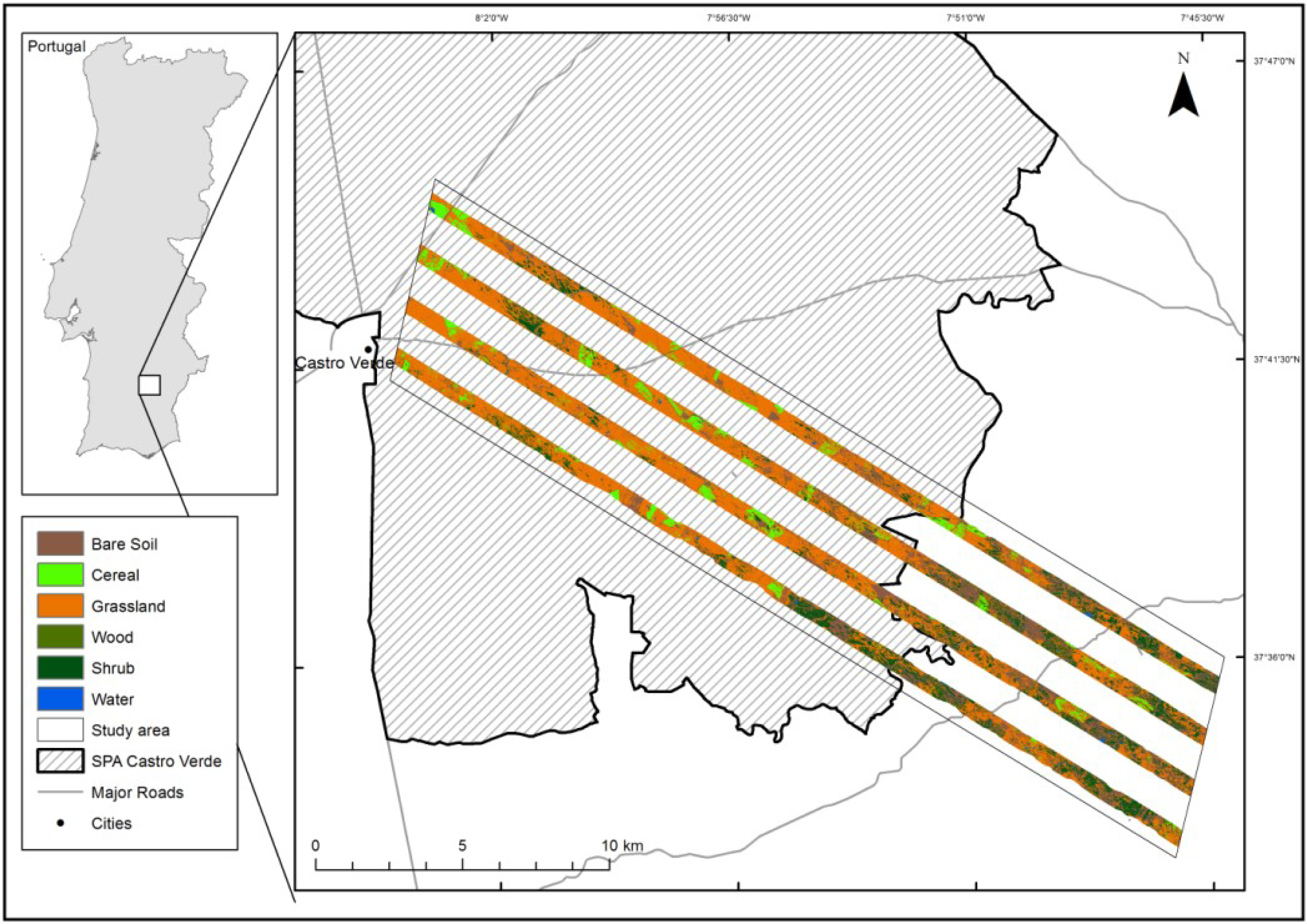
2.1. Study Area
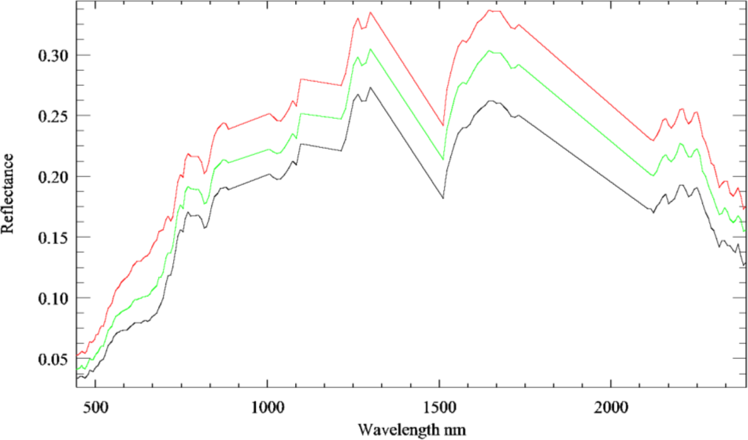
2.2. Data
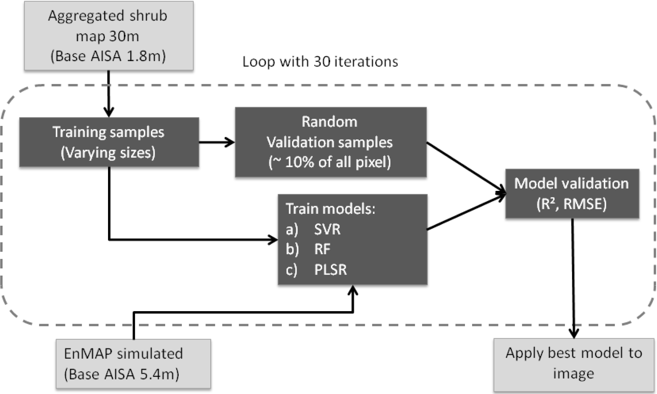
2.3. Data Analysis
2.3.1. Support Vector Regression
2.3.2. Random Forest Regression
2.3.3. Partial Least Squares Regression
3. Results
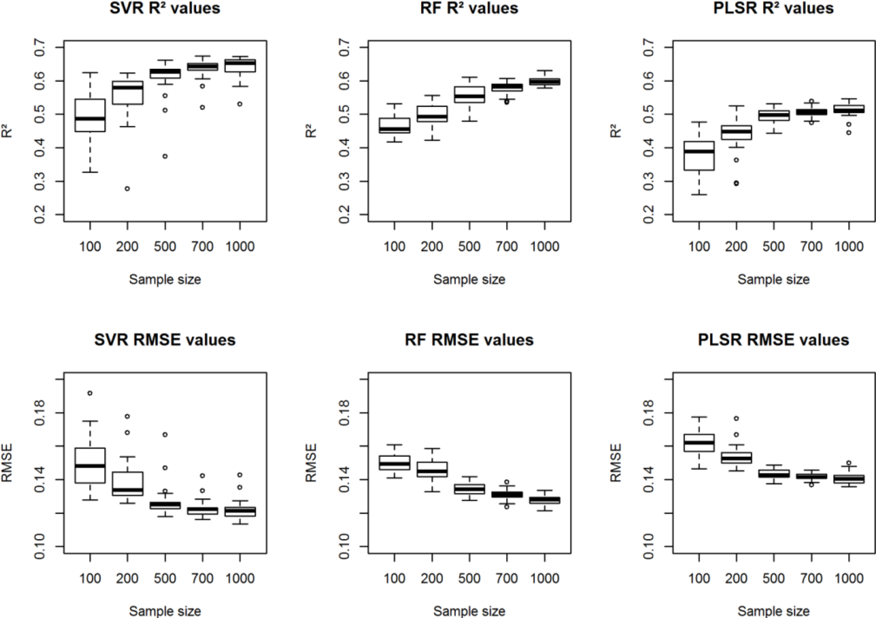
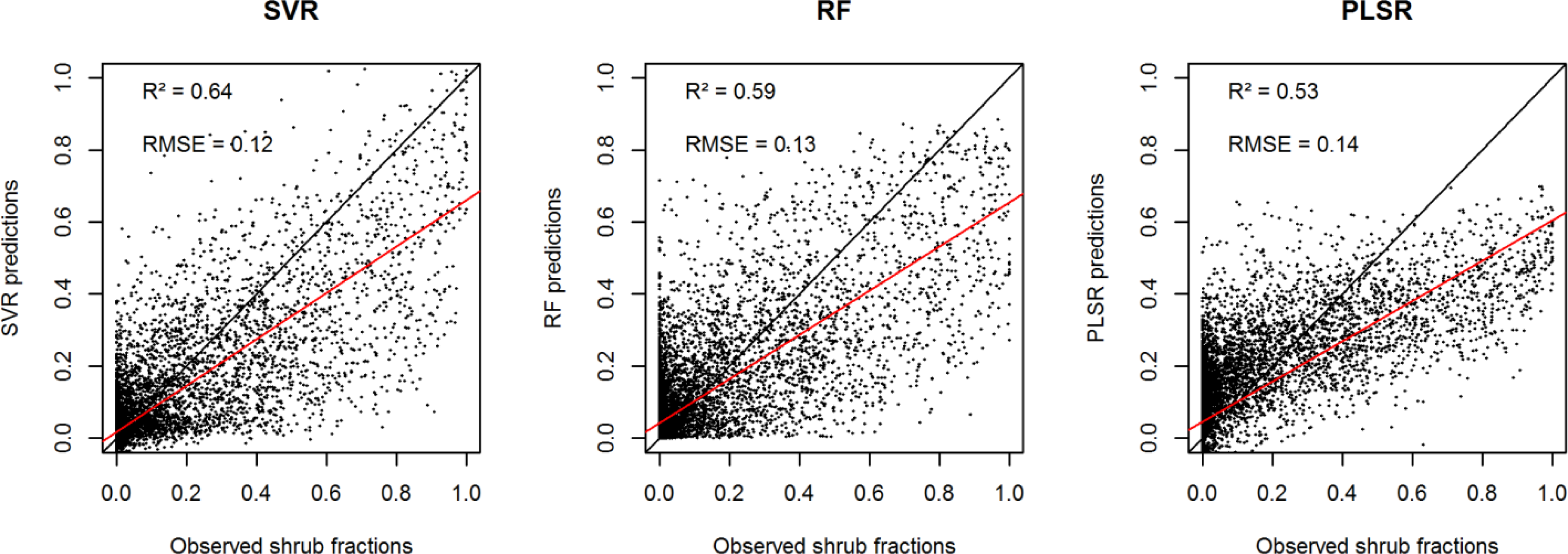
3.1. Regression Performance
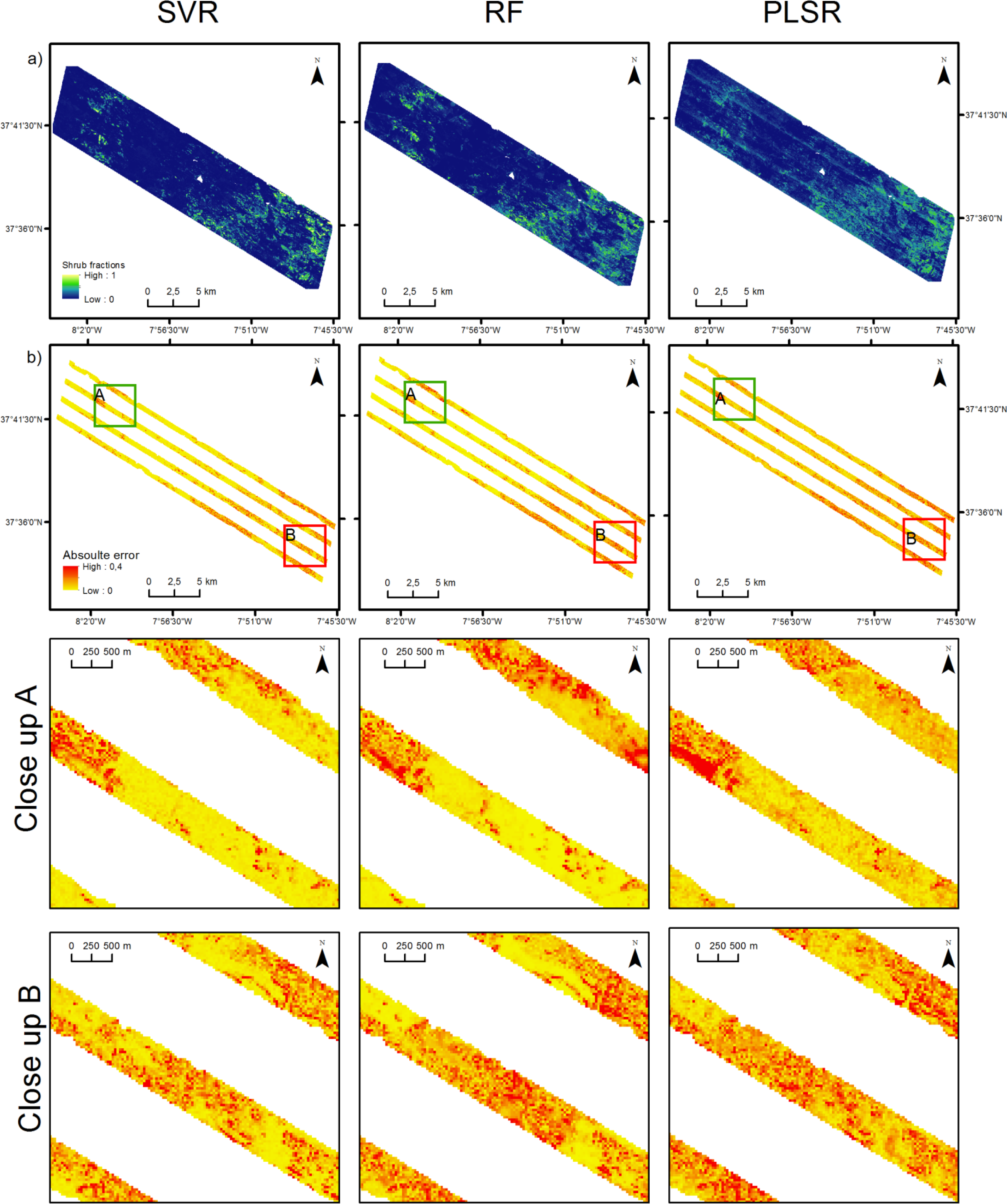
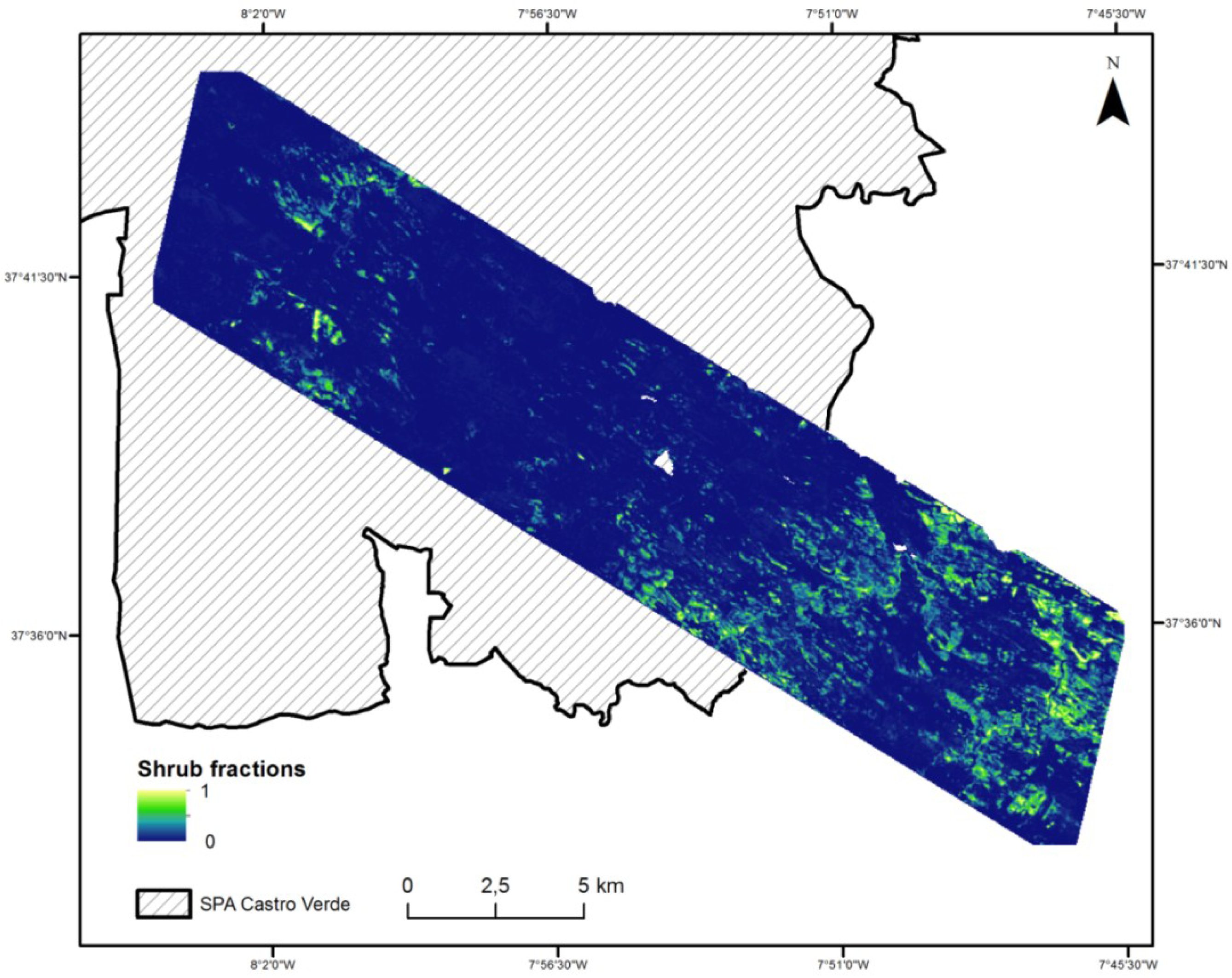
3.2. Spatial Pattern of Fractional Shrub Cover
4. Discussion
4.1. Comparison of Regression Algorithms
4.2. Training Sample Size
4.3. Uncertainty and Error Propagation
4.4. Predicted Spatial Patterns of Shrub Cover
5. Conclusions
Acknowledgments
Author Contributions
Conflicts of Interest
References
- Vitousek, P.M. Beyond global warming: Ecology and global change. Ecology 1994, 75, 1861–1876. [Google Scholar]
- Rey Benayas, J.; Martins, A.; Nicolau, J.M.; Schulz, J.J. Abandonment of agricultural land: An overview of drivers and consequences. CAB Rev.: Perspect. Agric. Vet. Sci. Nutr. Nat. Resour 2007, 2, 1–14. [Google Scholar]
- Millenium Ecosystem Assessment. Ecosystems and Human Well-Being: Synthesis; Island Press: Washington, DC, USA, 2005; p. 137. [Google Scholar]
- Eldridge, D.J.; Bowker, M.A.; Maestre, F.T.; Roger, E.; Reynolds, J.F.; Whitford, W.G. Impacts of shrub encroachment on ecosystem structure and functioning: Towards a global synthesis. Ecol. Lett 2011, 14, 709–722. [Google Scholar]
- Hill, J.; Hostert, P.; Tsiourlis, G.; Kasapidis, P.; Udelhoven, T.; Diemer, C. Monitoring 20 years of increased grazing impact on the Greek Island of Crete with earth observation satellites. J. Arid Environ 1998, 39, 165–178. [Google Scholar]
- Maestre, F.T.; Bowker, M.A.; Puche, M.D.; Belén Hinojosa, M.; Martínez, I.; García-Palacios, P.; Castillo, A.P.; Soliveres, S.; Luzuriaga, A.L.; Sánchez, A.M.; et al. Shrub encroachment can reverse desertification in semi-arid Mediterranean grasslands. Ecol. Lett 2009, 12, 930–941. [Google Scholar]
- Shoshany, M.; Karnibad, L. Mapping shrubland biomass along Mediterranean climatic gradients: The synergy of rainfall-based and NDVI-based models. Int. J. Remote Sens 2011, 32, 9497–9508. [Google Scholar]
- Van Auken, O.W. Shrub invasions of North American semiarid grasslands. Annu. Rev. Ecol. Syst 2000, 31, 197–215. [Google Scholar]
- Van Auken, O.W. Causes and consequences of woody plant encroachment into western North American grasslands. J. Environ. Manag 2009, 90, 2931–2942. [Google Scholar]
- Millenium Ecosystem Assessment. A Report of the Millennium Ecosystem Assessment. In Ecosystems and Human Well-Being: Desertification Synthesis; Island Press: Washington, DC, USA, 2005; p. 26. [Google Scholar]
- Fonseca, F.; Figueiredo, T.; Bompastor Ramos, M.A. Carbon storage in the Mediterranean upland shrub communities of Montesinho Natural Park, Northeast of Portugal. Agrofor. Syst 2012, 86, 463–475. [Google Scholar]
- Moreira, F.; Russo, D. Modelling the impact of agricultural abandonment and wildfires on vertebrate diversity in Mediterranean Europe. Landsc. Ecol 2007, 22, 1461–1476. [Google Scholar]
- Calvão, T.; Palmeirim, J.M. A comparative evaluation of spectral vegetation indices for the estimation of biophysical characteristics of Mediterranean semi-deciduous shrub communities. Int. J. Remote Sens 2011, 32, 2275–2296. [Google Scholar]
- Lambin, E.F.; Geist, H. Land-Use and Land-Cover Change: Local Processes and Global Impacts; Springer: Berlin, Germany, 2006. [Google Scholar]
- DeFries, R.; Pagiola, S.; Adamowicz, W.L.; Akcakaya, R.H.; Arcenas, A.; Babu, S.; Balk, D.; Confalonieri, U.; Cramer, W.; Falconi, F.; et al. Analytical Approaches for Assessing Ecosystem Condition and Human Well-Being. In Ecosystems and Human Well-Being: Current States and Trends; Hassan, R.M., Ed.; Island Press: Washington, DC, USA, 2005; pp. 37–71. [Google Scholar]
- Lawrence, R.L.; Wood, S.D.; Sheley, R.L. Mapping invasive plants using hyperspectral imagery and Breiman Cutler classifications (RandomForest). Remote Sens. Environ 2006, 100, 356–362. [Google Scholar]
- Thenkabail, P.S.; Enclona, E.A.; Ashton, M.S.; van der Meer, B. Accuracy assessments of hyperspectral waveband performance for vegetation analysis applications. Remote Sens. Environ 2004, 91, 354–376. [Google Scholar]
- Chopping, M.; Su, L.; Laliberte, A.; Rango, A.; Peters, D.P.C.; Kollikkathara, N. Mapping shrub abundance in desert grasslands using geometric-optical modeling and multi-angle remote sensing with CHRIS/PROBA. Remote Sens. Environ 2006, 104, 62–73. [Google Scholar]
- Stuffler, T.; Förster, K.; Hofer, S.; Leipold, M.; Sang, B.; Kaufmann, H.; Penné, B.; Mueller, A.; Chlebek, C. Hyperspectral imaging—An advanced instrument concept for the EnMAP mission (environmental mapping and analysis programme). Acta Astronaut 2009, 65, 1107–1112. [Google Scholar]
- Kaufmann, H. Science Plan of the Environmental Mapping and Analysis Program (EnMAP); Scientific Technical Report; Deutsches Geoforschungszentrum GFZ: Potsdam, Germany, 2012; p. 65. [Google Scholar]
- Storch, T.; Bachmann, M.; Eberle, S.; Habermeyer, M.; Makasy, C.; Miguel, A.; Mühle, H.; Müller, R. Enmap Ground Segment Design: An Overview and Its Hyperspectral Image Processing Chain. In Earth Observation for Global Change. Lecture Notes in Geoinformation and Cartography; Krisp, J.M., Meng, L., Pail, L., Stilla, U., Eds.; Springer: Heidelberg, Germany, 2013; pp. 49–62. [Google Scholar]
- Dormann, C.F.; Elith, J.; Bacher, S.; Buchmann, C.; Carl, G.; Carré, G.; Marquéz, J.R.G.; Gruber, B.; Lafourcade, B.; Leitão, P.J.; et al. Collinearity: A review of methods to deal with it and a simulation study evaluating their performance. Ecography 2013, 36, 27–46. [Google Scholar]
- Schölkopf, B.; Smola, A.J.; Williamson, R.C.; Bartlett, P.L. New support vector algorithms. Neural Comput 2000, 12, 1207–1245. [Google Scholar]
- Breiman, L. Random forests. Mach. Learn 2001, 45, 5–32. [Google Scholar]
- Wold, S.; Sjöström, M.; Eriksson, L. PLS-regression: A basic tool of chemometrics. Chemom. Intell. Lab. Syst 2001, 58, 109–130. [Google Scholar]
- Srivastava, A.N.; Oza, N.C.; Stroeve, J. Virtual sensors: Using data mining techniques to efficiently estimate remote sensing spectra. IEEE Trans. Geosci. Remote Sens 2005, 43, 590–599. [Google Scholar]
- Walton, J.T. Subpixel urban land cover estimation: Comparing Cubist, Random Forests, and support vector regression. Photogramm. Eng. Remote Sens 2008, 74, 1213–1222. [Google Scholar]
- Verrelst, J.; Muñoz, J.; Alonso, L.; Delegido, J.; Rivera, J.P.; Camps-Valls, G.; Moreno, J. Machine learning regression algorithms for biophysical parameter retrieval: Opportunities for Sentinel-2 and -3. Remote Sens. Environ 2012, 118, 127–139. [Google Scholar]
- Bajwa, S.G.; Kulkarni, S.S. Hyperspectral Data Mining. In Hyperspectral Remote Sensing of Vegetation; Thenkabail, P.S., Lyon, J.G., Huete, A., Eds.; CRC Press: Boca Raton, FL, USA, 2012; pp. 93–120. [Google Scholar]
- Leitão, P.J.; Moreira, F.; Osborne, P.E. Breeding habitat selection of steppe birds in Castro Verde: A remote sensing and advanced statistics approach. Ardeola 2010, 2010, 93–116. [Google Scholar]
- Doorn, A.M.; Pinto Correia, T. Differences in land cover interpretation in landscapes rich in cover gradients: Reflections based on the montado of South Portugal. Agrofor. Syst 2007, 70, 169–183. [Google Scholar]
- Delgado, A.; Moreira, F. Bird assemblages of an Iberian cereal steppe. Agric. Ecosyst. Environ 2000, 78, 65–76. [Google Scholar]
- Moreira, F.; Beja, P.; Morgado, R.; Reino, L.; Gordinho, L.; Delgado, A.; Borralho, R. Effects of field management and landscape context on grassland wintering birds in southern Portugal. Agric. Ecosyst. Environ 2005, 109, 59–74. [Google Scholar]
- Pereira, H.M.; Domingos, T.; Vicente, L. (Eds.) Portugal Millennium Ecosystem Assessment: State of the Assessment Report; Centro de Biologia Ambiental, Faculdade de Ciências da Universidade de Lisboa, 2004; p. 68. Available online: http://ecossistemas.org (accessed on 17 April 2014).
- Catry, I.; Franco, A.M.A.; Rocha, P.; Alcazar, R.; Reis, S.; Cordeiro, A.; Ventim, R.; Teodósio, J.; Moreira, F.; Chiaradia, A. Foraging habitat quality constrains effectiveness of artificial nest-site provisioning in reversing population declines in a colonial cavity nester. PLoS One 2013, 8, 1–10. [Google Scholar]
- Moreira, F. Relationships between vegetation structure and breeding bird densities in fallow cereal steppes in Castro Verde, Portugal. Bird Study 1999, 46, 309–318. [Google Scholar]
- Moreira, F.; Leitão, P.J.; Morgado, R.; Alcazar, R.; Cardoso, A.; Carrapato, C.; Delgado, A.; Geraldes, P.; Gordinho, L.; Henriques, I.; et al. Spatial distribution patterns, habitat correlates and population estimates of steppe birds in Castro Verde. Airo 2007, 5–30. [Google Scholar]
- Marta-Pedroso, C.; Domingos, T.; Freitas, H.; Groot, R.S. Cost-benefit analysis of the zonal program of Castro Verde (Portugal): Highlighting the trade-off between biodiversity and soil conservation. Soil Tillage Res 2007, 97, 79–90. [Google Scholar]
- Richter, R.; Schläpfer, D. Geo-atmospheric processing of airborne imaging spectrometry data. Part 2: Atmospheric/topographic correction. Int. J. Remote Sens 2002, 23, 2631–2649. [Google Scholar]
- Richter, R.; Schläpfer, D. Atmospheric/Topographic Correction for Airborne Imagery, Atcor-4 User Guide, Version 4.2. Remote Sensing Data Center, German Aerospace Center (DLR): Oberpfaffenhofen, Germany, 2007. Available online: http://dlr.de/ (accessed on 17 April 2014).
- Schläpfer, D.; Richter, R. Geo-atmospheric processing of airborne imaging spectrometry data. Part 1: Parametric orthorectification. Int. J. Remote Sens 2002, 23, 2609–2630. [Google Scholar]
- Segl, K.; Guanter, L.; Rogass, C.; Kuester, T.; Roessner, S.; Kaufmann, H.; Sang, B.; Mogulsky, V.; Hofer, S. Eetes—The EnMAP end-to-end simulation tool. IEEE J. Select. Top. Appl. Earth Obs. Remote Sens 2012, 5, 522–530. [Google Scholar]
- Olofsson, P.; Foody, G.M.; Stehman, S.V.; Woodcock, C.E. Making better use of accuracy data in land change studies: Estimating accuracy and area and quantifying uncertainty using stratified estimation. Remote Sens. Environ 2013, 129, 122–131. [Google Scholar]
- R Development Core Team. R: A Language and Environment for Statistical Computing. Available online: http://www.R-project.org (accessed on 17 April 2014).
- Brereton, R.G.; Lloyd, G.R. Support vector machines for classification and regression. Analyst 2010, 135, 230–267. [Google Scholar]
- Karatzoglou, A.; Meyer, D.; Hornik, K. Support vector machines in R. J. Stat. Softw 2006, 15, 2–28. [Google Scholar]
- Cortes, C.; Vapnik, V. Support-vector networks. Mach. Learn 1995, 20, 273–297. [Google Scholar]
- Smola, A.J.; Schölkopf, B. A tutorial on support vector regression. Stat. Comput 2004, 14, 199–222. [Google Scholar]
- Hornik, K.; Leisch, F.; Meyer, D.; Weingessel, A.; Dimitriadou, E. E1071: Misc Functions of the Department of Statistics (e1071); TU Wien: Vienna, Austria, 2010. [Google Scholar]
- Chang, C.-C.; Lin, C.-J. LIBSVM. ACM Trans. Intell. Syst. Technol 2011, 2, 1–27. [Google Scholar]
- Breiman, L.; Friedman, J.; Olshen, R.; Stone, C. Classification and Regression Trees; Wadsworth and Brooks: Belmont, CA, USA, 1984; p. 358. [Google Scholar]
- Liaw, A.; Wiener, M. Classifiaction and regression by randomForest. R News 2002, 2, 18–22. [Google Scholar]
- Mevik, B.-H.; Wehrens, R. The PLS package: Principal component and partial least squares regression in R. J. Stat. Softw 2007, 2, 1–24. [Google Scholar]
- Schmidtlein, S.; Oldenburg, C.; Feilhauer, H. R-Package AutoPLS: PLS Regression with Backward Selection of Predictors, Version 1.2-6; 2013. Available online: http://cran.r-project.org/ (accessed on 17 April 2014).
- Tuia, D.; Verrelst, J.; Alonso, L.; Perez-Cruz, F.; Camps-Valls, G. Multioutput support vector regression for remote sensing biophysical parameter estimation. IEEE Geosci. Remote Sens. Lett 2011, 8, 804–808. [Google Scholar]
- Leitão, P.J. Improving Species Distribution Models to Describe Steppe Bird Occurrence Patterns and Habitat Selection in Southern Portugal; Ph.D. Thesis, University of Southampton, Southampton, UK; 2008. [Google Scholar]
- Oldeland, J.; Dorigo, W.; Wesuls, D.; Jürgens, N. Mapping bush encroaching species by seasonal differences in hyperspectral imagery. Remote Sens 2010, 2, 1416–1438. [Google Scholar]


| R2 | RMSE | ||||||||||
|---|---|---|---|---|---|---|---|---|---|---|---|
| Sample Size | 100 | 200 | 500 | 700 | 1000 | 100 | 200 | 500 | 700 | 1000 | |
| SVR | Mean | 0.50 | 0.56 | 0.61 | 0.64 | 0.64 | 0.15 | 0.14 | 0.13 | 0.12 | 0.12 |
| Std. | 0.07 | 0.07 | 0.05 | 0.03 | 0.03 | 0.02 | 0.01 | 0.01 | 0.01 | 0.01 | |
| RF | Mean | 0.47 | 0.50 | 0.56 | 0.58 | 0.60 | 0.15 | 0.15 | 0.13 | 0.13 | 0.13 |
| Std. | 0.03 | 0.03 | 0.03 | 0.02 | 0.01 | 0.01 | 0.01 | 0.01 | 0.01 | 0.01 | |
| PLSR | Mean | 0.38 | 0.44 | 0.50 | 0.51 | 0.51 | 0.16 | 0.15 | 0.14 | 0.14 | 0.14 |
| Std. | 0.05 | 0.05 | 0.02 | 0.02 | 0.02 | 0.01 | 0.01 | 0.01 | 0.01 | 0.01 | |
© 2014 by the authors; licensee MDPI, Basel, Switzerland This article is an open access article distributed under the terms and conditions of the Creative Commons Attribution license (http://creativecommons.org/licenses/by/3.0/).
Share and Cite
Schwieder, M.; Leitão, P.J.; Suess, S.; Senf, C.; Hostert, P. Estimating Fractional Shrub Cover Using Simulated EnMAP Data: A Comparison of Three Machine Learning Regression Techniques. Remote Sens. 2014, 6, 3427-3445. https://doi.org/10.3390/rs6043427
Schwieder M, Leitão PJ, Suess S, Senf C, Hostert P. Estimating Fractional Shrub Cover Using Simulated EnMAP Data: A Comparison of Three Machine Learning Regression Techniques. Remote Sensing. 2014; 6(4):3427-3445. https://doi.org/10.3390/rs6043427
Chicago/Turabian StyleSchwieder, Marcel, Pedro J. Leitão, Stefan Suess, Cornelius Senf, and Patrick Hostert. 2014. "Estimating Fractional Shrub Cover Using Simulated EnMAP Data: A Comparison of Three Machine Learning Regression Techniques" Remote Sensing 6, no. 4: 3427-3445. https://doi.org/10.3390/rs6043427