Article

Rain-Use-Efficiency: What it Tells us about the Conflicting Sahel Greening and Sahelian Paradox

1
Geosciences Environnement Toulouse (GET), Observatoire Midi-Pyrénées, UMR 5563 (CNRS/UPS/IRD/CNES), 14 Avenue Edouard Belin, F-31400 Toulouse, France
2
Laboratoire des Sciences du Climat et de l'Environnement (LSCE), UMR 8212 (CNRS/CEA/UVSQ/), F-91190 Gif Sur Yvette, France
*
Author to whom correspondence should be addressed.
Remote Sens. 2014, 6(4), 3446-3474; https://doi.org/10.3390/rs6043446
Submission received: 16 January 2014 / Revised: 3 April 2014 / Accepted: 8 April 2014 / Published: 22 April 2014
(This article belongs to the Special Issue Monitoring Global Vegetation with AVHRR NDVI3g Data (1981-2011))

Abstract

:
Rain Use Efficiency (RUE), defined as Aboveground Net Primary Production (ANPP) divided by rainfall, is increasingly used to diagnose land degradation. Yet, the outcome of RUE monitoring has been much debated since opposite results were found about land degradation in the Sahel region. The debate is fueled by methodological issues, especially when using satellite remote sensing data to estimate ANPP, and by differences in the ecological interpretation. An alternative method which solves part of these issues relies on the residuals of ANPP regressed against rainfall (“ANPP residuals”). In this paper, we use long-term field observations of herbaceous vegetation mass collected in the Gourma region in Mali together with remote sensing data (GIMMS-3g Normalized Difference Vegetation Index) to estimate ANPP, RUE, and the ANPP residuals, over the period 1984–2010. The residuals as well as RUE do not reveal any trend over time over the Gourma region, implying that vegetation is resilient over that period, when data are aggregated at the Gourma scale. We find no conflict between field-derived and satellite-derived results in terms of trends. The nature (linearity) of the ANPP/rainfall relationship is investigated and is found to have no impact on the RUE and residuals interpretation. However, at odds with a stable RUE, an increased run-off coefficient has been observed in the area over the same period, pointing towards land degradation. The divergence of these two indicators of ecosystem resilience (stable RUE) and land degradation (increasing run-off coefficient) is referred to as the “second Sahelian paradox”. When shallow soils and deep soils are examined separately, high resilience is diagnosed on the deep soil sites. However, some of the shallow soils show signs of degradation, being characterized by decreasing vegetation cover and increasing run-off coefficient. Such results show that contrasted changes may co-exist within a region where a strong overall re-greening pattern is observed, highlighting that both the scale of observations and the scale of the processes have to be considered when performing assessments of vegetation changes and land degradation.

Graphical Abstract

1. Introduction

1.1. RUE and the Desertification/“Re-greening” Debate

Rain Use Efficiency is defined as the ratio between net primary production (NPP), or aboveground NPP (ANPP), and rainfall. It has been increasingly used to analyze the variability of vegetation production in arid and semi-arid biomes, where rainfall is a major limiting factor for plant growth [15]. Indeed, RUE was designed to separate rainfall contribution to vegetation production from other factors such as plant life-form, nutrient status or anthropogenic effects, like management and cropping practices [6]. For a given ecosystem preserved from any kind of functional change through time, the RUE values should be stable over time [6]. Thus, the underlying assumption is that a decline of RUE over time is a diagnosis for land degradation, or even “desertification” [4]. Since the 1980s, the increasing availability of remote sensing observations of vegetation cover, thanks to Earth Observation satellites, allowed estimating RUE over large areas and throughout long time periods. Thus, over the past decades the RUE index has been widely used to assess land degradation worldwide.
Although RUE is an appealing concept, both its derivation from satellite data and its interpretation in ecological terms present substantial difficulties, which fueled significant debates [7]. The case of the Sahel drought has given rise to such a debate with opposing theories and interpretations and several revisits of published findings [812]. Indeed, in the 1970s and 1980s, two successive and very severe droughts occurred in the Sahel, which had dramatic impact on the population and their resources. These extreme events, embedded in a long period of below-average rainfall, contributed to revive the vision of a Sahel suffering from desertification. Some of the most commonly cited causes of degradation comprise a climate-driven degradation of ecosystems (droughts) and land use changes, for instance changes in crop practices (over-exploitation of land, shortening of fallow duration), rangeland management (over-grazing), or extensive wood cutting (deforestation).
However, this hypothesis of an ongoing desertification process has been challenged over the last decades by several studies based on satellite observations that reported a spectacular “re-greening” of the Sahel, occurring since the beginning of satellite archive, that is the early 1980s [1317]. Cited causes of the re-greening ranged from climate variability (with a recovery of the rainfall amount) to improved farming techniques, and land reclamation.
Evidence from long-term ground data has shown that vegetation evolution is not uniform throughout the whole Sahel. Most regions show strong signs of “re-greening” trends, which can mostly be attributed to an increase in herbaceous production [17]. However, in other regions a decrease of vegetation production is undoubtedly taking place, even if it seems not to be widespread. For instance, decreasing vegetation production has been observed from both long-term ground data and satellite archive in south-western Niger [17].

1.2. The Sahelian Hydrological Paradox

Concurrently to the observation of a re-greening Sahel over the last decades, several studies showed that the run-off coefficient, defined as run-off divided by the rainfall amount, has dramatically increased from the 1950s up to now (for a review see Descroix et al. [18]; also refer to Mahe and Paturel [19] and references therein). In many places, the increased water table height fed by run-off (for instance in endoreic south-western Niger [20]), increased river run-off [21,22], increased pond surface [23], or increased flood of the Niger river [24] have been revealed after the strong droughts of the 1970s and 1980s. These phenomena are observed although rainfall decreased over the same period: this is known as the “Sahelian paradox” [25].
Over a few areas such as south-western Niger, the increase in run-off coefficient observed is in accordance with a decrease in vegetation cover [17,18], thus logically suggesting that an increase in the bare surfaces induce increasing run-off coefficient. However, in most regions of Sahel, the increasing run-off coefficient contradicts the general re-greening trends reported.
As increasing run-off coefficient is also considered a consequence of land degradation [26], another paradoxical situation emerges. How can vegetation productivity increase while at the same time run-off coefficient increases? A good understanding of how net primary productivity relates to rainfall is required to solve this “second Sahelian paradox”.

1.3. Limitations Related to Methodological Issues

Several studies have explored the changes in Sahelian RUE over the last decades, reaching contrasted conclusions. While some point towards land degradation [9], others conclude to the absence of extensive land degradation [8,15,27]. The differences in interpretation partly result from methodological issues, and partly from different ecological theories or expectations.
As far as methods are concerned, the RUE concept is based on proportionality between ANPP and rainfall [6]. This approach is meaningful when ANPP reaches zero when rainfall also reaches zero (i.e., zero intercept) [28]. This may not be the case when, for instance, NDVI (which is slightly positive for bare soils) instead of ANPP is used in RUE calculation, or if a rainfall threshold is needed for the vegetation to start growing [28,29]. In both cases, the non-zero intercept will cause RUE to artificially tend to infinity values at very low rainfall. Thus, when calculating the trends of RUE over time, significant trends will emerge if rainfall undergoes temporal changes within this range of values. Such trends cannot be interpreted as changes in the ecosystem’s functioning since they are only caused by mathematical artifacts.
Different methods have been proposed to remove methodological difficulties (see Fensholt et al. [27] for a review). For instance, Fensholt et al. [27] only retained pixels with a strong correlation between satellite NDVI and annual rainfall, but with no significant correlation between RUE and rainfall. Regressing ANPP against rainfall, as suggested by Evans and Geerken [30] for instance, alleviates the non-zero intercept problems. The slope of the linear regression is a first useful indicator of the ANPP/rainfall relationship, also referred to as the Precipitation Marginal Response (PMR) [28,31]. A second indicator derived from this relationship is the difference between “predicted ANPP” (from rainfall) and observed ANPP. In the following text, this method will be referred to as the “ANPP residuals” method.
By construction, if one assumes that the relationship between ANPP and rainfall is linear, the ANPP residuals are independent from rainfall. Therefore, significant temporal trends in the residuals truly show changes in vegetation production which are not related to rainfall. These trends in the residuals may be positive or negative, and reflect changes in vegetation composition, land cover (to name a few), and finally indicate land degradation [4]. Moreover, the ANPP residuals can be examined to look for a non-random distribution and possible dependency of residuals on rainfall amount [2,7,27,30]. Indeed, if the hypothesis of a linear relationship between ANPP and rainfall does not hold, it should be evidenced by the shape of the distribution of RUE plotted against rainfall. The ANPP residuals approach is usually recommended rather than the RUE one. In this study, however, both methods are investigated so that possible false interpretations found with the widely used RUE method can be identified.
However, the residuals method is also subject to some limitations. Wessels et al. [32] analyzed the performance of ordinary least-square regressions (OLS) to detect land degradation, by simulating various scenarios of land degradation with a 16-year-long time series. Among other factors, they investigated the influence of the timing of the degradation, i.e., whether it happens at the beginning, middle, or end of the time series, and its intensity, by testing a range of degradation from 20% to 40%. In addition to showing that iNDVI needs to be reduced by 30% to 40% before significant negative trends can be detected, they showed that land degradation happening at the beginning or at the end of the time series are usually undetected. Furthermore, their results suggest that the residuals method (called RESTREND in their paper) becomes unsuitable for a simulated degradation intensity greater that 20%, since beyond this threshold the relationship between ANPP and rainfall breaks down.

1.4. Limitations Related to Ecological Interpretation

On the ecological side of the controversy (is land degradation diagnosed from the temporal changes in RUE in the Sahel?) the key question is the dependency of RUE on rainfall. The situation occurs if the ANPP/rainfall relationship departs from proportionality.
First, this can happen if RUE is intrinsically lower for higher rainfall amounts, which has been suggested several times based on field observations (e.g., Miehe et al. [33], Hein and de Ridder [9], Ruppert et al. [2]). In that case, an increase in rainfall would be accompanied by a decrease in RUE, without any land degradation. A similar situation may affect the other edge of the rainfall range: if RUE increases with rainfall (because for instance RUE is intrinsically low for the lowest rainfall), a recovery of the rainfall should result in increasing RUE [2,9].
Therefore, in the specific context of the Sahel region, the rainfall increase after the 1980s drought should lead to a decrease in RUE, without being attributable to any widespread “desertification”. Relying on that hypothesis and on a few field observations, Hein and de Ridder [9] argued that the lack of significant increase in Sahelian RUE over the 1984–2000 period had to be interpreted as an evidence of widespread desertification of the whole Sahelian region. But Prince et al. [12] and Miehe [11] in turn challenged their hypothesis and results. They both advocated linearity of the ANPP/rainfall relationship, then found either stable or increasing RUE trends over most parts of the Sahel region, and finally concluded that no widespread desertification was threatening the Sahel. Therefore, interpreting the RUE temporal changes requires prior investigation of the proportionality of the ANPP/rainfall relationship (or linearity for the ANPP residuals) as well as verification of the hypothesis of no dependency of RUE to rainfall.

1.5. Limitations Related to the Data Used

As it is common for long-term ecological studies, other issues may arise because of inaccuracies related to the rainfall and ANPP data themselves. In addition, estimating ANPP over large regions requires up-scaling of ground data using remote sensing methods. The Normalized Difference Vegetation Index (NDVI) is particularly used to estimate ANPP and to perform RUE analyses [8,15,29,3436], most often without being calibrated over ground measurements of ANPP.
In water-limited regions, the NDVI/ANPP relationship has been firmly established, from both empirical studies [37,38] and theoretical ones [39]. The latter is generally built on the “Monteith model”, which states that NDVI linearly correlates with the fraction of photosynthetically active radiation absorbed by plants (fPAR), which in turn correlates with photosynthesis, and, after integration in time, to ANPP [40]. These relationships are known to vary in space and time depending on vegetation type, but this variability is significantly reduced when focusing of one single type of ecosystem, which is the case in our study. The slope of the APAR/ANPP relationship is referred to as the Light Use Efficiency (LUE), APAR being the absorbed photosynthetically active radiation. This approach has proven very successful over the years. However, it is recognized that uncertainty affects the different terms of the Monteith model and especially the LUE, which may depend on plant type, phenology, water, temperature or nutrient stresses.
In addition, the derivation of long series of NDVI needs to solve a number of problems like orbital drift, changing atmospheric conditions, sensor degradation [41]. As a result, the accuracy of long-term estimates of ANPP derived from NDVI is not well-known, especially for biomes where long-term ground data are scarce. Given these uncertainties, it is certainly important to evaluate long-term time series of RUE and ANPP residuals with corresponding long-term ground data [17,33,36].

1.6. Mains Objectives of this Study

The present study focuses on the temporal changes of the herbaceous vegetation cover in the Gourma region in Mali, where 27 years of field observations of the aboveground herbaceous mass are available. A strong re-greening pattern is observed using both field data and remote-sensing measurements [17]; a re-greening that we aim to understand through the analysis of RUE and ANPP residuals.
This study addresses the three main following questions:
(i)
The first methodological goal will be to evaluate the use of remote sensing NDVI data to estimate indicators of land degradation such as RUE and ANPP residuals. The consistency within these two methods (RUE and residuals) will be examined as well.
(ii)
The second objective is to understand whether the re-greening trends observed over the Gourma region can be explained by rainfall.
(iii)
Then, this study investigates how re-greening and increased run-off coefficient can be observed in the same region: an explanation of the “second Sahelian paradox” that reconciles increased run-off coefficient and overall re-greening trends will be proposed.

2. Data and Methods

2.1. Field Observations of Vegetation
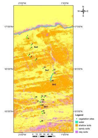
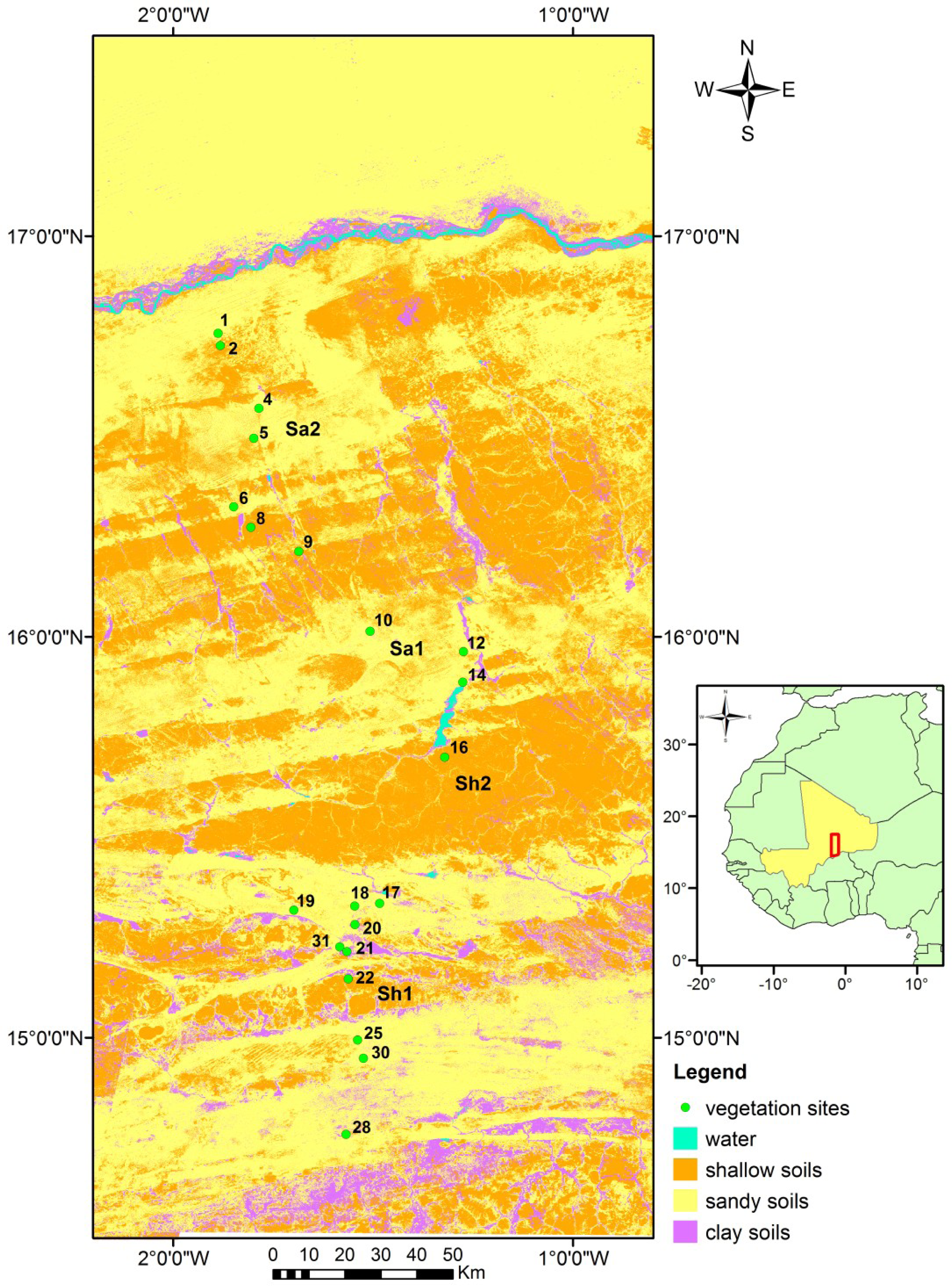
2.1.1. Study Area

The Gourma region is located in north-eastern Mali, south of the Niger River. The exact area considered in this study extends from 14.5 to 17.5°N and from 2.2 to 0.8°W, and will be referred to hereafter as the “Gourma window”. Field observations of aboveground herbaceous vegetation mass are available from 1984 to 2010. The Gourma is a pastoral region, land under cultivation representing less than 5% of the surface. The vegetation is mainly constituted of annual herbaceous plants, the woody plants covering less than 3% of the surface. Twenty-one sites of 1 km2 have been used in this study, which were measured every year for 27 years, at least when the field campaigns could be performed (some temporal gaps in the dataset do exist, but sites irregularly measured apart from these gaps have not been used). These twenty-one sites (Figure 1) sample the bioclimatic gradient of the Gourma region (annual rainfall ranging from 140 mm at the northern edge of the Gourma window, to 470 mm at the southern edge; Frappart et al. [42]) as well as the landscape heterogeneity: soil type, water regime, topography, land use, grazing pressure intensity [43].

2.1.2. Sampling Strategy

Herbaceous ANPP is derived from the aboveground herbaceous mass measured for each site through a stratified random sampling method [17,44]. The stratification stage was built to take into account the variability in aboveground herbaceous vegetation density at the site scale. Four classes (the “strata”) are defined following the vegetation density: bare soil, low-density, middle-density and high-density. The frequency of each stratum at the site scale is estimated along a 1 km line, by classifying the 1 m × 1 m plots into the 4 strata previously defined. Destructive measurements are performed over a few plots (3 for the low and high density strata, 6 for the middle one, which is also the more frequent), which were randomly selected along the line. For these plots, herbaceous plants are cut, dried, and weighted. Finally, a weighted average relying on the stratification provides the aboveground herbaceous mass at the site level.

2.1.3. ANPP Estimation

Dardel et al. [17] analyzed the time series of ground ANPP averaged at the Gourma window scale in relation to the GIMMS-3g time series, using peak mass as a proxy for ANPP. In this study, ANPP estimation is further refined. First, more severe criteria are used to select sites without significant temporal gaps (thus selecting 21 sites over the 38 available in the database). For instance, sites with only a few years of measurements available (either because the site monitoring was abandoned or because it started lately) are set aside.
Second, for some sites which are sampled more often than others (mostly because of their ease of access), several measurements per year are performed. It is thus possible to detect when the mass goes through several maxima during the growing season. This occurs, although rarely, when a strong dry spell interrupts plant growth. In that case ANPP is best approximated by the sum of the successive mass increments rather than by the mass maximum [45]. This correction was applied in this study, even though the impact on ANPP estimate is small since the vegetation is dominated by annual plants growing rapidly during a short rain season. Finally, we also compensated for late measurements of mass, assuming an average rate of mass decay of 17% per month (based on field data) and a maximum of standing mass in mid-September. This occurred principally for year 1995. Still, differences between our estimates and real ANPP may be caused by mass losses caused by herbivory, which is not taken into account.

2.1.4. Spatial Average
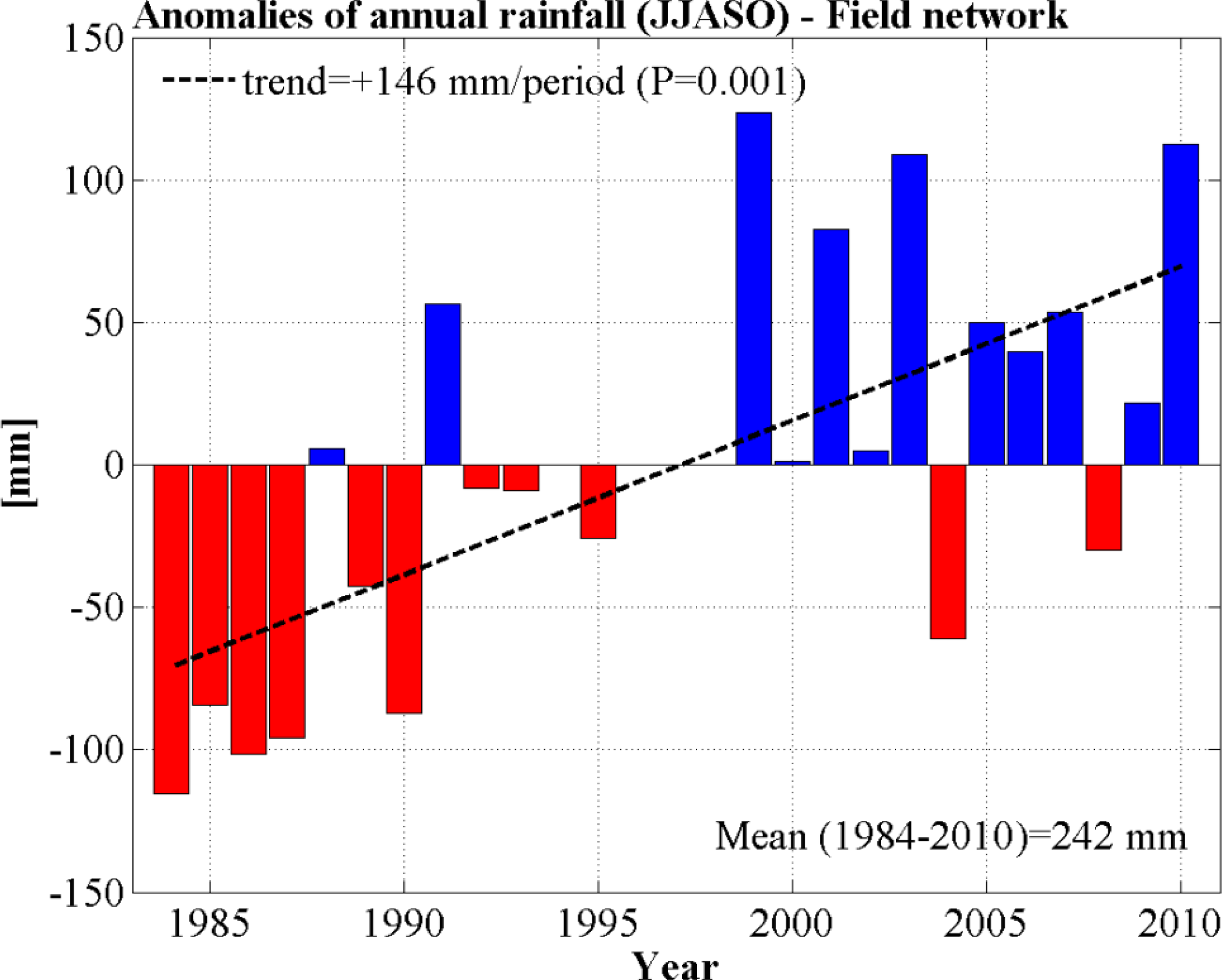
Since the field data are collected over areas significantly smaller than the GIMMS-3g satellite pixels, we chose to average both field data and satellite data over a relatively large window (3° × 1.2°). The field sites are grouped following the three main soil types characterizing the Gourma region: deep sandy soils, shallow soils and clayed depressions (Figure 1). Indeed, soil type is a main driver of vegetation production in the Gourma, as shown in Dardel et al. [17] (Figure 10) and in Hiernaux et al. [44] (Figure 5 and Table 3). Therefore, an average ANPP for the Gourma window is obtained by weighting ANPP by the respective proportion of these three main soil types (coefficients derived from a supervised classification from Landsat images): 65.1% of sandy surfaces, 30.8% of shallow soils, and 4.1% of clayed depressions. We therefore focus on the temporal changes of ANPP and RUE of a relatively large area.

2.2. Rainfall Data

Studies of RUE preferably rely on rainfall data collected by ground networks, but rain gauge data are scarce and of varying reliability in the Gourma region of Sahel. At the regional scale, gridded rainfall products combining rain gauge measurements with satellite data can be used [29]. Here, rainfall data come from a research network of rain gauges installed over the Gourma region [42]. Daily data available from 1984 up to 2010 have been quality-checked to discard gauges with spurious gaps, which occasionally occurs for isolated visual reading gauges or pluviographs. Sums for the June-July-August-September-October (JJASO) period were calculated for each gauge, and spatially averaged to provide one annual value for the Gourma window (Figure 2). Summing over the JJASO period allows catching most of the annual rainfall that is useful for herbaceous vegetation growth.
Most of the years, a rain gauge could be associated with every vegetation site, meaning that there was a gauge with good quality data close enough, typically within 10 km of the vegetation site. The Gourma average JJASO rainfall was compared to the simple average of the two long-term stations of Gourma-Rharous (station from Direction Nationale de la Météorologie du Mali, DNM) and Hombori (SYNOP station from DNM Mali). Also, to evaluate the use of satellite-based rainfall datasets in estimating RUE or ANPP residuals, we included the TARCAT v2.0 dataset from the TAMSAT Research Group (Tropical Applications of Meteorology using SATellite data and ground-based observations, Maidment et al. [46]). TARCAT provides rainfall estimates from 1983 up to today with a spatial resolution of 0.0375°, based on Meteosat thermal infra-red data and calibrated with ground-based rain gauge data. It aims at providing consistent estimations of rainfall over Africa for long-term studies since the calibration is constant over time for a given grid cell. In the rest of the manuscript, the baseline rainfall dataset is the one based on the network of gauges in the Gourma region. The sensitivity of the results to the different rainfall products is reported in Appendix A.

2.3. Normalized Difference Vegetation Index Data

2.3.1. The NDVI GIMMS-3g Dataset

The NDVI-3g dataset is produced by the Global Inventory Modeling and Mapping Studies (GIMMS) group from data collected with the AVHRR (Advanced Very High Resolution Radiometer) sensors, which have been carried out by polar-orbiting meteorological satellites from the NOAA (National Oceanic and Atmospheric Administration), and are currently flying onboard the MetOps 1 and 2 satellites. The GIMMS-3g dataset extends the widely used GIMMS dataset, which is available over the 1981–2006 period [41]. NDVI-3g data are provided globally from 1981 to 2012 with a 1/12° spatial resolution and 15-days maximum value composite images [47].
The GIMMS-3g NDVI is produced using a similar processing scheme than for the GIMMS dataset. NDVI data are calculated from the AVHRR channel 1 (red, 550–700 nm) and channel 2 (near-infrared, 730–1000 nm) reflectances. Calibration of the channel 1 and channel 2 reflectances is performed using the atmospheric Rayleigh scattering over oceans method of Vermote and Kaufman [48]; calibration of the NDVI itself is performed using the technique of Los [49], which relies on spectrally invariant targets such as desert areas, and finally artificial trends due to orbital drift are corrected using the empirical mode decomposition/recomposition (EMD) technique of Pinzon et al. [50], which separates the trends due to a varying solar zenith angle from the overall signal. No atmospheric correction is applied, except for the aerosol content due to the volcanic eruptions of El Chinchon (1982) and Mt Pinatubo (1991). In the GIMMS-3g dataset, another stage was implemented in the processing because of the dual gain introduced in the late 2000s with the first AVHRR/3 instrument. SeaWIFS NDVI data from 1997 to 2010 are used to calibrate the GIMMS-3g NDVI data, using Bayesian methods [47]. Thus, GIMMS-3g NDVI is the longest available dataset of vegetation cover available worldwide at a bi-monthly frequency, which provides a unique opportunity to perform trends and interannual variability analyses over more than 30 years.

2.3.2. Temporal and Spatial Aggregation

Seasonal NDVI integrals, noted hereafter iNDVI [51], were calculated on a per-pixel basis as follows: (i) the base level for integration was estimated as the dry season NDVI average (January to April, and November to December); (ii) a “normalized NDVI” was calculated for each year by subtracting the average dry season value from the original data; (iii) temporal integration of “normalized NDVI” was then applied over the growing season (July to October).
Finally a spatial average was calculated over the Gourma window. Indeed, even though it is not technically correct to average values obtained from a ratio, the difference with averaging the reflectances themselves is negligible (not shown). Besides, it was proven that performing a spatial average of the 9-km wide AVHRR pixels further reduces uncertainties [52].
For comparison, MODIS (MOD13C2) NDVI data were used as well during the 2000–2010 period, the data being available on a monthly basis with a spatial resolution of 0.05°. MODIS NDVI was integrated over the JJASO growing season and spatially averaged over the Gourma window, just like the GIMMS-3g data. The results obtained using MODIS are reported in Appendix B.

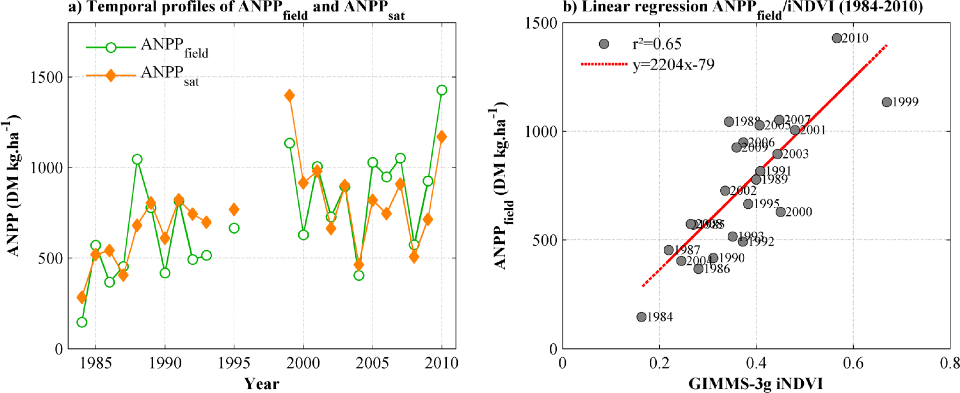
2.4. Estimation of Satellite-Derived ANPP

Satellite-derived ANPP is estimated by calibrating spatially averaged iNDVI on the multi-site weighted average ANPP observations (hereafter called “ANPPfield”), as explained in Section 2.1. The same method was used in Dardel et al. [17], except that the average over the growing season (August–September) was used, instead of iNDVI in the present study. Therefore, iNDVI is regressed against ANPPfield over 1984–2010, with iNDVI as the independent variable (Equation (1)),
ANP P field = a × iNDVI + b + ɛ
where a is the slope of the regression, b the intercept, and ɛ an error term.
The resulting linear regression coefficients (a, b) are in turn used to provide satellite estimates of ANPP from iNDVI, referred to as “ANPPsat” (Equation (2)),
ANPP sat = a × iNDVI + b
The same method was applied over 2000–2010, using iNDVI data from both GIMMS-3g and MODIS. Time series of ANPPfield and ANPPsat are described in detail in Dardel et al. [17]. The focus here is on the relationships between these series and the rainfall series, using linear regression (Ordinary Least Square regression) and Principal Component Analysis of z-scores of the three series.
As ANPPsat is simply obtained as a linear scaling of iNDVI, most analyses can be equally performed using either iNDVI or ANPPsat. When calculating rain use efficiencies however, only ANPPsat should be used, to avoid the methodological issues described before (non-zero intercept, see Section 1.3).

2.5. Calculation of Rain Use Efficiency and ANPP Residuals

Two time-series of Rain Use Efficiency are calculated as the ratio of spatially averaged ANPPfield and ANPPsat, respectively, to annual rainfall, over the Gourma window. These time-series are referred to as “RUEfield” and “RUEsat”.
The ANPP residuals method is also applied to both field observations and satellite estimates. First, a linear regression between ANPP estimates (field or satellite) and annual rainfall is calculated, providing the “predicted ANPP” (field or satellite) time series. ANPP residuals are then calculated as the difference between observed ANPP and predicted ANPP, and are referred to as “field residuals” and “satellite residuals” for field observations and satellite data, respectively.
Temporal trends over the period 1984–2010 are calculated using Ordinary Least-Square regressions for each of these datasets (RUEfield, RUEsat, field residuals, satellite residuals). Their relationship with rainfall is examined as well.

3. Results and Discussion

3.1. Limitations Related to ANPP Estimation from iNDVI

A number of issues may impair the derivation of ANPP from long time series of AVHRR data, which did not aim originally at monitoring vegetation, and thus require significant challenges to be overcome before vegetation cover trends can be successfully derived (succession of 10 sensors, calibration issues, band width, atmospheric long-term variability, orbital drift, to name a few). While these data are processed to minimize all these perturbations [47], the impact on the ANPP/iNDVI relation is not easily quantified. Many factors are known to influence this relationship (soil background and color, grazing pressure, floristic composition, land use and land cover, etc.), but neither their direct effect nor their temporal changes are clearly known [17]. The overall consistency of the precipitation time series with both field ANPP and satellite ANPP can be seen as an evaluation of the whole data processing involved.

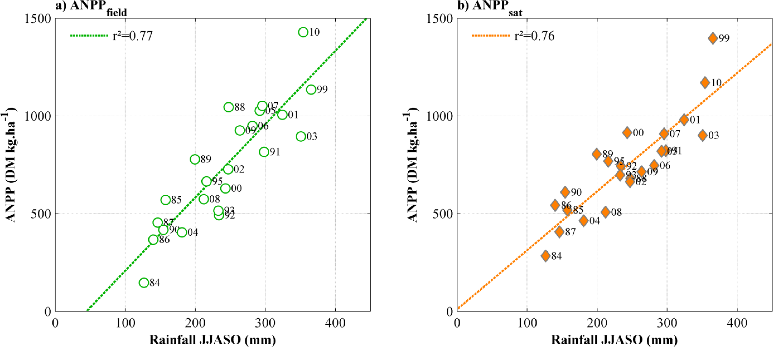
3.2. ANPP and Rainfall

Over the 1984–2010 period, satellite-derived ANPP and field-derived ANPP vary in a very consistent way (Figure 3a). The temporal variations of both ANPPfield and ANPPsat show a recovery of plant production after the 1984’s drought, characterized by an increasing trend and a strong interannual variability. Field ANPP explains 65% of the iNDVI variance (Figure 3b), which is slightly higher than the 56% reported in Dardel et al. [17] for the correlation between peak biomass and NDVI over 1984–2011. Improvements in the estimation of ANPPfield, together with the use of a remote-sensing proxy for ANPPsat which is closer to the Monteith production model (iNDVI instead of the average over August–September), are most probably causing this. The agreement between the two datasets is better during the 2000–2010 period (r2 = 0.71, p = 0.0001) than during the 1984–1995 period (r2 = 0.48, p = 0.018). When Equations (1) and (2) are applied to estimate ANPP from MODIS and GIMMS-3g over 2000–2010, the temporal profiles of the three ANPP datasets are very similar and the explained variance reaches 87% for MODIS and 67% for GIMMS-3g (see Appendix B).
Whether ANPP is estimated from field data or from satellite GIMMS-3g NDVI data, it is highly correlated with the JJASO rainfall, which, in both cases, explains 76%–77% of the variance (Figure 4a,b). The overall consistency of the three datasets, each of which could be impaired by quality issues, therefore strongly supports the use of satellite NDVI archive for long-term monitoring of dry lands.

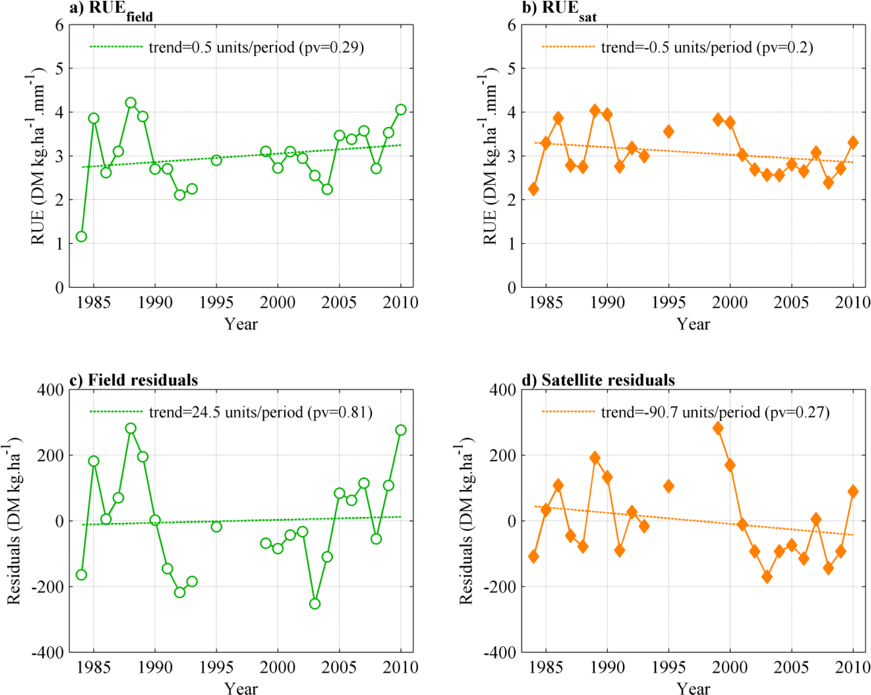
3.3. RUE and Residuals Interannual Variability and Trends

The relationship between field-derived ANPP and rainfall is illustrated by the temporal evolution of RUE and ANPP residuals over 1984–2010 (Figure 5a,c): RUEfield displays a low value in 1984, followed by a series of relatively high but variable RUE (or positive residuals) in 1985–1989, and then a rapid decrease from 1988 to 1992 followed by a slow recovery until 2010. Over the whole period, neither RUEfield nor field ANPP residuals show significant trends (p values of 0.29 and 0.81, respectively). The trend in RUEfield (non-significant) is in fact due to one single very low value observed in 1984. Noticeably, an analysis of RUEfield short-term trends starting after 1992 may suggest an increase in RUE. This again illustrates that trends have to be established over long periods of time and have to be robust over several time periods [17,33].
When RUE and ANPP residuals are based on satellite-derived ANPP (instead of ANPPfield), results also support a non-significant trend over 1984–2010 (Figure 5b,d). However, the temporal profiles of RUEsat lack the succession of high and low RUE anomalies detected with RUEfield, and the interannual variability does not correspond well to the one of RUEfield, except when the MODIS data are considered (see Appendix B).
These results are still valid when TAMSAT or the two-stations rainfall datasets (Hombori and Gourma-Rharous) are used instead of the Gourma rain-gauge network co-located with each vegetation site: no significant trends over the whole 1984–2010 period are detected for field- or satellite-derived RUE (or residuals), and similar slight differences in the shape of field and satellite RUE (or residuals) temporal profiles are found (see Appendix A). Thus, both methods present consistent results in terms of temporal trends over the Gourma region, when data (field or satellite) are aggregated at the window scale.

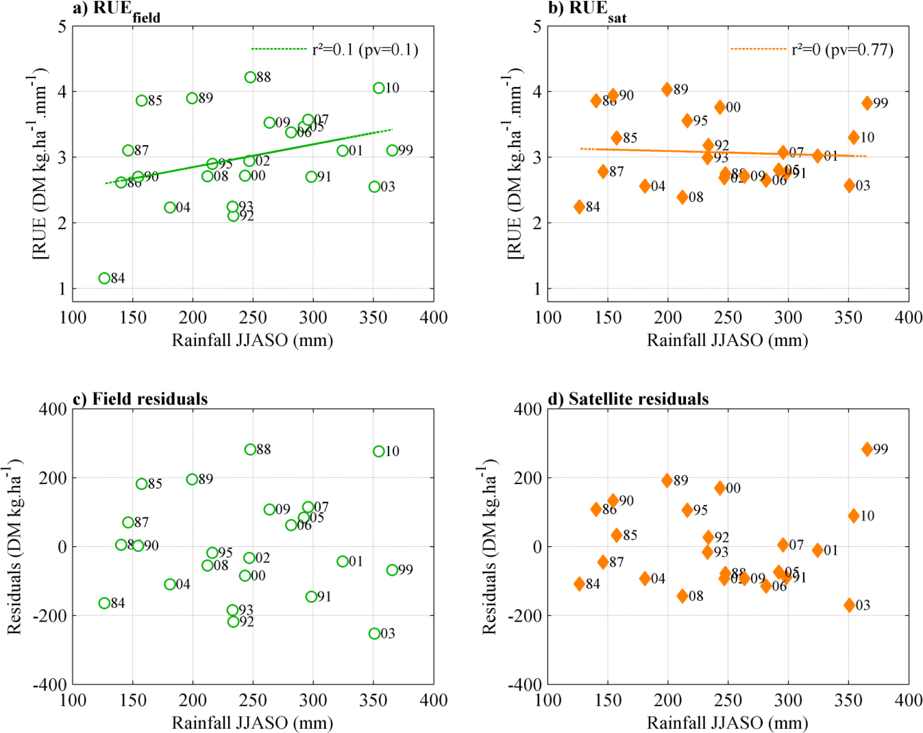
3.4. RUE and ANPP Residuals in Relation to Rainfall Amount

By construction, RUE and rainfall are not independent (see Section 1.3). As a result, the correlation between these two variables is prone to “spurious correlation”. For instance, Brett [53] showed that a small negative correlation between X/Y and Y is likely to occur, if X and Y are unrelated, depending on the variation coefficient of Y. In the case of RUE, a large coefficient of variation of rainfall may produce a slightly negative and spurious correlation.
For the Gourma region, RUEfield is slightly and positively correlated to rainfall (r2 = 0.1; Figure 6a). The correlation is significant at the 90% level (p = 0.10) but is caused by year 1984 only. On the other hand, the field residuals do not display any particular pattern when plotted against rainfall (Figure 6c), showing no support for non-linearity of the ANPP/rainfall relationship over the range of rainfall considered here. The highest rainfall values result in proportionally high ANPP, with no evidence of other factors (like nutrient status, being increasingly limiting when the water constraint is relieved). When looking at the results obtained with satellite-derived ANPP, RUEsat is not correlated to rainfall and the satellite residuals do not suggest either any non-linear relationship between ANPP and rainfall (Figure 6b,d).
The principal component analysis among ANPPfield, ANPPsat and rainfall supports the following statement: the three variables (ANPPfield, ANPPsat and rainfall) are strongly correlated. RUE or the residuals of ANPP versus rainfall are second order signals, which do not display significant trends over 1984–2010. Indeed, the first principal component explains 90% of the total variance, and the coefficients are similar for the three variables (0.57, 0.57, 0.59 for ANPPfield, ANPPsat and rainfall respectively). The second principal component explains 6% of the total variance, and the coefficients (0.71, −0.70, 0.01) indicate that it depicts the differences between ANPPfield and ANPPsat.
Therefore, over the Gourma region we find no conflict between the RUE approach and the ANPP residuals method, both in terms of temporal trends and when looking at their relationship with rainfall. Both data sources (i.e., field data and satellite observations) give consistent results, indicating that long-term satellite datasets can be used to monitor RUE (or residuals) over long time periods.

3.5. Ecological Interpretation

3.5.1. Comparison to Literature

It is well known that rainfall controls plant productivity in many ecosystems, and especially in semi-arid ecosystems such as in the Sahel. Herbaceous productivity in the Gourma is largely predicted by rain season rainfall amount. The range of RUE values found in this study is comparable to the range reported by studies in similar ecosystems [2,8,54,55]. Le Houerou [54], for instance, reported RUE between 1 and 4 DM·kg·ha−1·mm−1 for regions with mean annual precipitation around 250 mm (Saharo-Sahelian transition) and RUE values in the range of 1.7 to 8 DM·kg·ha−1·mm−1 for regions with mean annual precipitation around 350 mm. The ratio of field measurements of ANPP to annual rainfall typically ranges from 3 to 6 [33,36].
Correlation between satellite-derived ANPP (usually based on NDVI) or field ANPP and rainfall has been reported in the past for semi-arid regions. The strongest relationships are usually established when average ANPP is estimated along large climatic gradients. For example, r2 as high as 0.89 was reported for climatic means ranging from 200 to 800 mm·yr−1 in North America in Muldavin et al. [56], or 0.90 for a 200–1200 mm·yr−1gradient in Sala et al. [57]. The correlation based on interannual variability is usually much lower (Diouf and Lambin [36]: r2 = 0.41; Evans and Geerken [30]: r2 = 0.50 to 0.77, depending on the method used to estimate rainfall; Prince et al. [8]: r2 = 0.52; Muldavin et al. [56]: r2 = 0.56 to 0.66). Spatial averaging tends to increase the correlation: Nicholson et al. [34] found a correlation of 0.85 (r2) between Sahel-averaged NDVI and rainfall, for years 1982–1993. For our dataset, the variance explained by rainfall for both ANPPsat (76%) and ANPPfield (77%) is, therefore, in the upper values of the literature range. The spatial averaging method, although it is performed here over a much smaller area than Nicholson et al. [34], may contribute to reduce the noise in the data (but aggregation may also rise up-scaling issues and require adequate sampling; Holm et al. [58]).

3.5.2. Interannual Variability

Different ecological factors may cause variability in RUE and ANPP residuals [4]. Field data suggest that ANPP residuals may be negative in dry years as in 1984, 2004, 2008 (Figure 5c). Such a decrease is consistent with the idea that below a certain rainfall threshold (generally involving strong dry spells), vegetation growth may be more severely impaired, for instance if a large mortality event occurs during the rainy season, or if the drought limits resource capture (e.g., LAI) or resource use. Increased herbivory impact in poor production years may also lead to an underestimation of ANPP from mass data [33]. Such a drop of RUE for the driest years has also been shown in the meta-analysis of field data by Ruppert et al. [2]. However, some other dry years like 1985, 1987, or 1990 do not support this concept. In line with Miehe et al. [33], we do not find any clear delayed effect of the 1984 drought since high RUE and positive residuals are found as early as 1985. This is not in line with the lag effect of drought suggested by Prince et al. [8], Prince et al. [12] and Diouf and Lambin [36].

3.5.3. Ecosystems Resilience

The fact that no trend of RUE or ANPP residuals are found either from field data or satellite data demonstrates the resilience of ecosystems in the Gourma region, at least at that aggregated spatial scale. In other words, no degradation could be detected using these indicators.
However, Wessels et al. [32] suggested that a 30% to 40% decrease in ANPP is needed to be detected with a 16-year-long time series. Here, we used a 23-year-long dataset spanning a 27-year-long period. Similar simulations than the ones performed by Wessels et al. [32] (not detailed here) suggest that a degradation of 20% to 30% may be detected with our time series, provided they do not occur at the beginning or end of the series.
Keeping these limits in mind, we can conclude that in situ observations and satellite-based estimates of ANPP support the conclusions that the pastoral Gourma fully benefited from the rainfall increase over the last three decades, showing a global pattern of vegetation regeneration after the droughts, when the data are spatially aggregated.

3.6. Reconciling Stable RUE and Increasing Run-off Coefficient

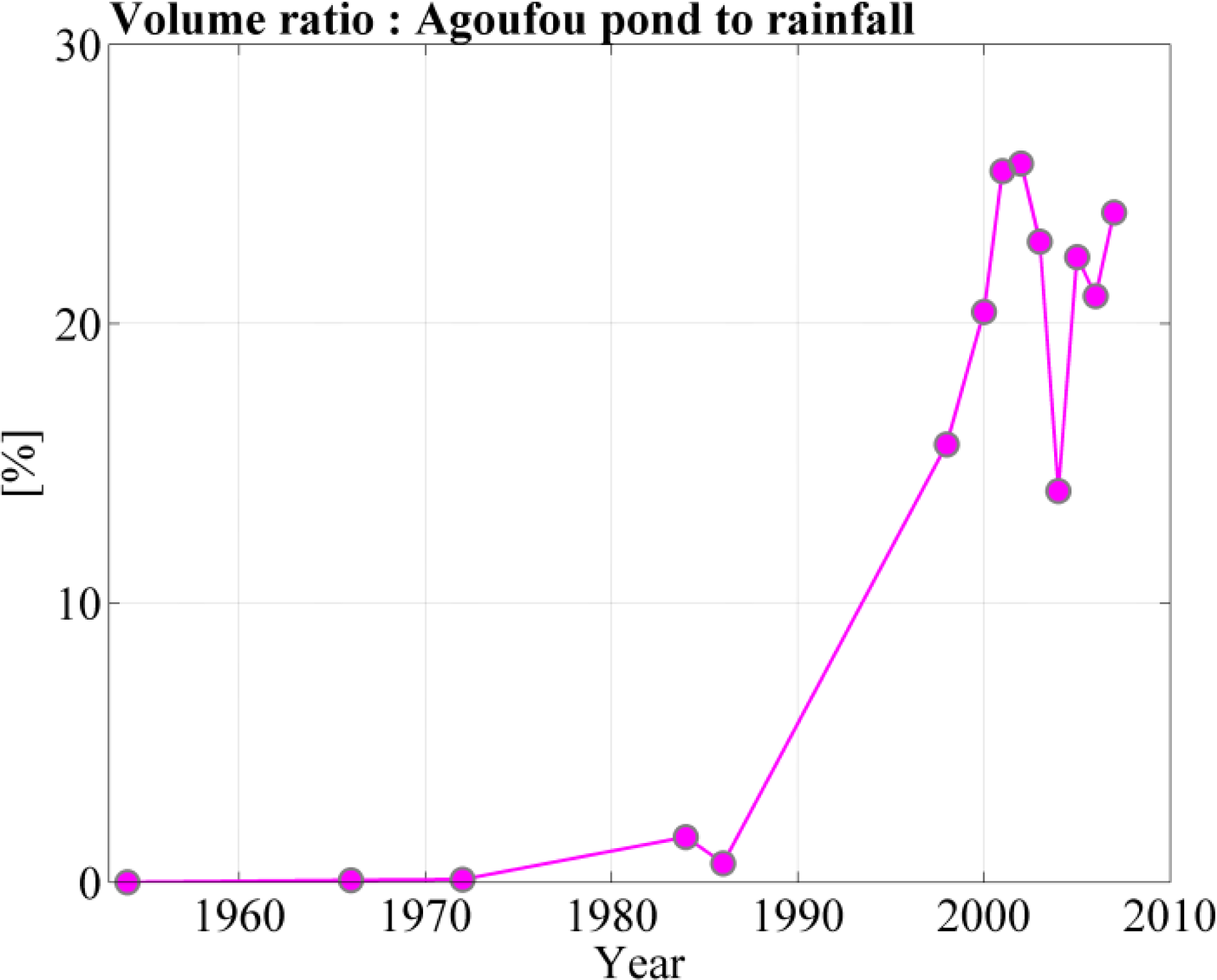
3.6.1. The Hydrological Sahelian Paradox in the Gourma Region

The results shown above make a strong case for stable RUE over 1984–2010 in the Gourma region, suggesting ecosystem resilience to water utilization. Yet, there is also compelling evidence that the run-off coefficient over the same area has dramatically increased over the same period (see Section 1.2). In fact, Gardelle et al. [23] demonstrated that most ponds in the Gourma started to grow after the 1970s drought, with an important acceleration of the phenomenon usually a few years after the 1983–1984 drought. The case of the Agoufou pond (located near sites 17, 18, 20 and 31 in Figure 1) illustrates this phenomenon (see also Haas et al. [59]). The annual increase of pond’s volume derived from Landsat and other high resolution imagery is a proxy of the water entering the pond, and therefore of the run-off collected over the catchment. The ratio of this volume to the annual precipitation rapidly increased after 1984, as can be seen in Figure 7 (100% increase was detected for all 91 ponds in the Gourma).
Local observations (like the growth of the gully network) support a significant trend towards run-off concentration and acceleration on some shallow soils, especially in the first years with normal or above-average rainfall after a major drought, like for example year 1991. Such an increase in run-off coefficient is often associated with land degradation, which is apparently conflicting with the stable RUE (and residuals) found over the same period.

3.6.2. Focus on the Shallow Soils Behavior

A detailed examination of shallow soils sites, however, shed some light on this question. The resolution of the GIMMS-3g data prevented strict comparisons of satellite data to specific sites since most sites are homogeneous at the 1 km scale but not at the 1/12° scale. Yet, several areas dominated by shallow soils or deep sandy soils are large enough to be observed with GIMMS-3g data. A typical shallow soil signal is obtained by averaging GIMMS-3g data over areas labeled “Sh1” and “Sh2” on Figure 1, and compared to a sandy soil signal averaged over the neighboring “Sa1” and “Sa2” areas, also shown on Figure 1. Hereafter only the results obtained with the ANPP residuals method are shown since the results obtained using the RUE index lead to similar conclusions.
Over the two units of deep sandy soils analyzed (Sa1 and Sa2), the spatially averaged iNDVI is strongly increasing over the whole period (Figure 8a), while satellite residuals are stable (Figure 8b), as they are over the whole Gourma region. The same signal is found with the field data available within the same zone (Figure 8c,d). Thus, the deep sandy soils exhibit the same resilience as the Gourma region when considered as a whole.
By contrast, over the neighboring shallow soils (Sh1 and Sh2), the spatially averaged iNDVI displays no trend over 1984–2010 (Figure 9a), whereas the satellite residuals display a weakly significant decreasing trend (p = 0.1, Figure 9b).
However, field data for two specific shallow soil sites, which are located into (site n°16) or close to (site n°8) the Sh1 and Sh2 areas, reveal contrasted behaviors (Figure 10). On site n°16, ANPPfield progressively recovers after the driest years (Figure 10a), while field residuals are stable over time (Figure 10b), implying that this given site behaves like the sandy soil sites although its productivity is much lower.
Conversely, for site n°8, ANPPfield at the end of the 1984–2010 period is much lower than in 1986–1990 (Figure 10a). ANPPfield time series reveal very low ANPP values for every year after 2005 (no observations being available between 1995 and 2005). Field trip reports mentioned soil erosion and run-off concentration in the early 1990s, which added limitations to plant growth for this site. The field residuals decrease as well (Figure 10b), the trend being close to significance (p = 0.11). However, in that case, the correlation between ANPP and rainfall disappears (r2 = 0.01; p = 0.7). This occurs when the changes in vegetation function are large, for instance in the case of intense degradation [32]. Therefore, the trend of the residuals comes close to the trend of ANPP, limiting the efficiency of the residuals method to detect vegetation cover changes that are not related to precipitation. It may still be possible to give an interpretation in terms of degradation, but a careful examination of all series, and especially precipitation, has to be performed. These conclusions are supported by the analysis of Veron et al. [4], who recommended the use of the RUE index (or the ANPP residuals) in conjunction with the PMR (Precipitation Marginal Response, Veron et al. [28]) and average ANPP to analyze land degradation.
Therefore, the response of the shallow soils ecosystems to the drought is not uniform. A similar analysis performed with the field data collected over site n°22 (located on Figure 1) resulted in insignificant trends, either in ANPPfield or in field residuals, thus showing an “intermediate behavior” between site n°8 and site n°16.
Shallow soil sites in the Gourma region typically consist of bedrock (schist or sandstone) or iron pan outcrops, interspersed with shallow patches of sand, sandy loam or clay loam, over which herbaceous vegetation and shrubs may grow [60]. Run-off is high from the rock or iron pan outcrops, and was most often occurring as sheet run-off that progressively evolved towards a more concentrated run-off in a web of rills and gullies. The sandy-loam patches are classically long shaped set perpendicular to the slope, separated by bare soil impluviums, creating the patterned vegetation locally known as “tiger bush”, where vegetated patches are able to capture sheet run-off. Nowadays, some of the shallow soil sites show clear signs of degradation, while others do not. In fact, all shallow soils suffered from the 1984’s drought, but this degradation was intensified over some sites only. In addition to herbaceous productivity, woody cover for these sites also tend to decay, as they have been deprived of water because of run-off concentration [61].

3.6.3. Reconciling Re-greening and the Sahelian Hydrological Paradox

Field data suggest that some of the shallow soil areas are prone to “degradation” (in the sense of decreasing ANPP), while others are less affected, or not affected at all. Since ponds’ water originates from the shallow soils only [23,62], degradation of a fraction of these landscape units is sufficient to cause a strong increase in run-off at the scale of the whole Gourma. The satellite-derived RUE and ANPP residuals are consistent with this different response of ANPP between shallow and sandy soils since they suggest decreasing ANPP residuals (and RUE, not shown) over the shallow soils areas Sh1 and Sh2 (Figure 9).
Thus, our results suggest that land degradation and increasing run-off coefficient can happen over very small surfaces, yet having tremendous hydrological impact at the regional scale. The re-greening observed at a wider scale remains indisputable, but our results highlight the fact that contrasted changes may happen at a smaller spatial scale (i.e., smaller than the GIMMS-3g pixel resolution), meaning that both the scale of observations and the finer scale of the processes have to be scrutinized when performing assessments of vegetation changes, and more importantly when assessing land degradation.
Besides, shallow soils in the Gourma region are relatively large landscape units, which may not be the case of iron pans or rocky outcrops in many other parts of the Sahel. Therefore, a slight decrease of productivity or RUE in areas of already low productivity (or RUE) would most probably be undetected in many places where shallow soils exist at a smaller spatial scale than the GIMMS-3g resolution [58]. Consequently, in situations where local degradation and erosion occur over a small fraction of a landscape, on patches surrounded by otherwise resilient re-greening ecosystems, both a stable RUE and an increasing run-off coefficient can be observed. Since increasing run-off coefficient is observed in many places in the Sahel and since the present study gives more confidence in RUE observed from space, which is often stable [27], we propose that divergent indicators of degradation may co-exist in the Sahel as soon as shallow soils are present, especially if their detection is complicated by a typical patch size smaller than the resolution of the remote sensing dataset.

4. Conclusions

Long-term ecological surveys provide strong evidence that the longest global satellite archive can be used to estimate aboveground net primary production (ANPP) over decades. Interannual variability of ANPP in pastoral Gourma (north-eastern Mali) and temporal trends following the extreme drought of the early 1980s are both consistently portrayed by ground and remote sensing time series, when aggregated over the 3° × 1.2° Gourma area. Both series are remarkably correlated to rainfall over 1984–2010, in a linear way. The residuals of ANPP regressed against rainfall as well as the Rain Use Efficiency (RUE) time series do not reveal any significant trend over time, implying that vegetation is resilient over that period at the Gourma scale, and that land degradation is not affecting the area at this level of aggregation. We found no conflict between field-derived and satellite-derived results in terms of trends and no role of non-linearity of the ANPP/rainfall relationship impacting the interpretation, two issues which are highly disputed.
At the same time, an increase in run-off coefficient has affected the same area over the period, pointing towards some land degradation. The apparent discrepancy of these two indicators of land degradation (stable RUE and increasing run-off coefficient) is referred to as the “second Sahelian paradox”. When shallow soils and deep soils were examined separately, high resilience was diagnosed on the deep sandy soil sites, but the shallow soils either showed signs of resilience or degradation. We argue that the “second Sahelian paradox” observed in the Gourma region can be explained by the fact that the small fraction of the landscape showing signs of degradation is dominated, in terms of ANPP, by the large fraction of resilient and productive deep sandy soils. We suggest that similar processes may exist in many other dry lands, as soon as some shallow soils are present and are not scrutinized separately.
Thus, these “Sahelian paradoxes” seem more related to an observation shortcoming than to an actual paradox. It reflects that global studies analyzing changes in vegetation cover at continental to regional scales may miss local-scale changes such as the ones highlighted in this study. Global patterns of re-greening may actually hide real changes in the eco-hydrological processes, yet concerning a very small fraction of the landscape, but leading to tremendous modifications of the hydrological systems. A more complete picture of the actual changes happening in the Sahel region could be achieved by taking into account these scaling issues. As we hypothesize that the shallow soils present all over the Sahel may experience consequent changes such as the ones observed in the Gourma region, we suggest to perform further investigation over similar soils continent-wide. High resolution imagery (such as Landsat or airborne images) could be used to assess whether these eco-hydrological changes are affecting a larger extent of the region.

Acknowledgments

We thank the anonymous reviewers for their in-depth analyses, very valuable remarks and suggestions. This work was funded by ANR ESCAPE (ANR-10-CEPL-005) and used data from Service d’Observation AMMA-CATCH and from DNM Mali. First author was funded by the CNES (Centre National d’Études Spatiales) and by the Midi-Pyrénées Region. We thank Jim Tucker and Assaf Anyamba for making the GIMMS-3g data available, and Marielle Gosset for helpful discussions on TARCAT. Finally, we thank all the people involved in the field measurements all over the years.

Authors Contributions

Cécile Dardel and Laurent Kergoat designed the sudy, performed the data analysis and wrote the manuscript. Pierre Hiernaux and Eric Mougin designed the observation network, provided data and assisted in their analysis. Manuela Grippa and Philippe Ciais contributed to the data analysis and interpretation. Cam-Chi Nguyen provided the Gourma soil type map.

Conflicts of Interest

The authors declare no conflict of interest.

References

  1. Huxman, T.E.; Smith, M.D.; Fay, P.A.; Knapp, A.K.; Shaw, M.R.; Loik, M.E.; Smith, S.D.; Tissue, D.T.; Zak, J.C.; Weltzin, J.F.; et al. Convergence across biomes to a common rain-use efficiency. Nature 2004, 429, 651–654. [Google Scholar]
  2. Ruppert, J.C.; Holm, A.; Miehe, S.; Muldavin, E.; Snyman, H.A.; Wesche, K.; Linstadter, A. Meta-analysis of ANPP and rain-use efficiency confirms indicative value for degradation and supports non-linear response along precipitation gradients in drylands. J. Veg. Sci 2012, 23, 1035–1050. [Google Scholar]
  3. Fensholt, R.; Rasmussen, K.; Nielsen, T.T.; Mbow, C. Evaluation of earth observation based long term vegetation trends—Intercomparing NDVI time series trend analysis consistency of Sahel from AVHRR GIMMS, Terra MODIS and SPOT VGT data. Remote Sens. Environ 2009, 113, 1886–1898. [Google Scholar]
  4. Veron, S.R.; Paruelo, J.M.; Oesterheld, M. Assessing desertification. J. Arid. Environ 2006, 66, 751–763. [Google Scholar]
  5. Bai, Y.F.; Wu, J.G.; Xing, Q.; Pan, Q.M.; Huang, J.H.; Yang, D.L.; Han, X.G. Primary production and rain use efficiency across a precipitation gradient on the Mongolia plateau. Ecology 2008, 89, 2140–2153. [Google Scholar]
  6. Le Houerou, H.N. Rain use efficiency—A unifying concept in arid-land ecology. J. Arid. Environ 1984, 7, 213–247. [Google Scholar]
  7. Wessels, K.J. Comments on “Proxy global assessment of land degradation” by Bai et al. (2008). Soil Use Manag 2009, 25, 91–92. [Google Scholar]
  8. Prince, S.D.; de Colstoun, E.B.; Kravitz, L.L. Evidence from rain-use efficiencies does not indicate extensive Sahelian desertification. Glob. Chang. Biol 1998, 4, 359–374. [Google Scholar]
  9. Hein, L.; de Ridder, N. Desertification in the Sahel: A reinterpretation. Glob. Chang. Biol 2006, 12, 751–758. [Google Scholar]
  10. Hein, L.; de Ridder, N.; Hiernaux, P.; Leemans, R.; de Wit, A.; Schaepman, M. Desertification in the Sahel: Towards better accounting for ecosystem dynamics in the interpretation of remote sensing images. J. Arid. Environ 2011, 75, 1164–1172. [Google Scholar]
  11. Miehe, S. Comment on: Hein, L. 2006: The impacts of grazing and rainfall variability on the dynamics of a Sahelian rangeland. J. Arid. Environ 2006, 64, 488–504. [Google Scholar]
  12. Prince, S.D.; Wessels, K.J.; Tucker, C.J.; Nicholson, S.E. Desertification in the Sahel: A reinterpretation of a reinterpretation. Glob. Chang. Biol 2007, 13, 1308–1313. [Google Scholar]
  13. Eklundh, L.; Olsson, L. Vegetation index trends for the African Sahel 1982–1999. Geophys. Res. Lett 2003, 30, 1430–1433. [Google Scholar]
  14. Anyamba, A.; Tucker, C.J. Analysis of Sahelian vegetation dynamics using NOAA-AVHRR NDVI data from 1981–2003. J. Arid. Environ 2005, 63, 596–614. [Google Scholar]
  15. Herrmann, S.M.; Anyamba, A.; Tucker, C.J. Recent trends in vegetation dynamics in the African Sahel and their relationship to climate. Glob. Environ. Chang.-Hum. Policy Dimens 2005, 15, 394–404. [Google Scholar]
  16. Fensholt, R.; Proud, S.R. Evaluation of Earth Observation based global long term vegetation trends—Comparing GIMMS and MODIS global NDVI time series. Remote Sens. Environ 2012, 119, 131–147. [Google Scholar]
  17. Dardel, C.; Kergoat, L.; Hiernaux, P.; Mougin, E.; Grippa, M.; Tucker, C.J. Re-greening Sahel: 30 years of remote sensing data and field observations (Mali, Niger). Remote Sens. Environ 2014, 140, 350–364. [Google Scholar]
  18. Descroix, L.; Mahe, G.; Lebel, T.; Favreau, G.; Galle, S.; Gautier, E.; Olivry, J.C.; Albergel, J.; Amogu, O.; Cappelaere, B.; et al. Spatio-temporal variability of hydrological regimes around the boundaries between Sahelian and Sudanian areas of West Africa: A synthesis. J. Hydrol 2009, 375, 90–102. [Google Scholar]
  19. Mahe, G.; Paturel, J.E. Sahelian annual rainfall variability and runoff increase of Sahelian Rivers. Comptes Rendus Geosci 2009, 341. [Google Scholar]
  20. Leduc, C.; Favreau, G.; Schroeter, P. Long-term rise in a sahelian water-table: The Continental Terminal in South-West Niger. J. Hydrol 2001, 243, 43–54. [Google Scholar]
  21. Amogu, O.; Descroix, L.; Yero, K.S.; le Breton, E.; Mamadou, I.; Ali, A.; Vischel, T.; Bader, J.C.; Moussa, I.B.; Gautier, E.; et al. Increasing river flows in the Sahel? Water 2010, 2, 170–199. [Google Scholar]
  22. Descroix, L.; Laurent, J.P.; Vauclin, M.; Amogu, O.; Boubkraoui, S.; Ibrahim, B.; Galle, S.; Cappelaere, B.; Bousquet, S.; Mamadou, I.; et al. Experimental evidence of deep infiltration under sandy flats and gullies in the Sahel. J. Hydrol 2012, 424, 1–15. [Google Scholar]
  23. Gardelle, J.; Hiernaux, P.; Kergoat, L.; Grippa, M. Less rain, more water in ponds: A remote sensing study of the dynamics of surface waters from 1950 to present in pastoral Sahel (Gourma region, Mali). Hydrol. Earth Syst. Sci 2010, 14, 309–324. [Google Scholar]
  24. Sighomnou, D.; Descroix, L.; Genthon, P.; Mahé, G.; Bouzou Moussa, I.; Gautier, E.; Mamadou, I.; Vandervaere, J.P.; Bachir, T.; Coulibaly, B.; et al. La crue de 2012 à Niamey: Un paroxysme du paradoxe du Sahel? Sécheresse 2013, 24, 3–13. [Google Scholar]
  25. Albergel, J. The influence of Climate Change and Climatic Variability on the Hydrologic Regime and Water Resources. In Sécheresse, Désertification et Ressources en Eau de Surface: Application Aux petits Bassins du BURKINA FASO; IAHS Publisher: Vancouver, BC, Canada, 1987; pp. 355–365. [Google Scholar]
  26. Savenije, H.H.G. The runoff coefficient as the key to moisture recycling. J. Hydrol 1996, 176, 219–225. [Google Scholar]
  27. Fensholt, R.; Rasmussen, K.; Kaspersen, P.; Huber, S.; Horion, S.; Swinnen, E. Assessing land degradation/recovery in the african sahel from long-term earth observation based primary productivity and precipitation relationships. Remote Sens 2013, 5, 664–686. [Google Scholar]
  28. Veron, S.R.; Oesterheld, M.; Paruelo, J.M. Production as a function of resource availability: Slopes and efficiencies are different. J. Veg. Sci 2005, 16, 351–354. [Google Scholar]
  29. Fensholt, R.; Rasmussen, K. Analysis of trends in the Sahelian “rain-use efficiency” using GIMMS NDVI, RFE and GPCP rainfall data. Remote Sens. Environ 2011, 115, 438–451. [Google Scholar]
  30. Evans, J.; Geerken, R. Discrimination between climate and human-induced dryland degradation. J. Arid. Environ 2004, 57, 535–554. [Google Scholar]
  31. Begue, A.; Vintrou, E.; Ruelland, D.; Claden, M.; Dessay, N. Can a 25-year trend in Soudano-Sahelian vegetation dynamics be interpreted in terms of land use change? A remote sensing approach. Glob. Environ. Chang 2011, 21, 413–420. [Google Scholar]
  32. Wessels, K.J.; van den Bergh, F.; Scholes, R.J. Limits to detectability of land degradation by trend analysis of vegetation index data. Remote Sens. Environ 2012, 125, 10–22. [Google Scholar]
  33. Miehe, S.; Kluge, J.; von Wehrden, H.; Retzer, V. Long-term degradation of Sahelian rangeland detected by 27 years of field study in Senegal. J. Appl. Ecol 2010, 47, 692–700. [Google Scholar]
  34. Nicholson, S.E.; Tucker, C.J.; Ba, M.B. Desertification, drought, and surface vegetation: An example from the West African Sahel. Bull. Am. Meteorol. Soc 1998, 79, 815–829. [Google Scholar]
  35. Wessels, K.J.; Prince, S.D.; Malherbe, J.; Small, J.; Frost, P.E.; VanZyl, D. Can human-induced land degradation be distinguished from the effects of rainfall variability? A case study in South Africa. J. Arid. Environ 2007, 68, 271–297. [Google Scholar]
  36. Diouf, A.; Lambin, E.F. Monitoring land-cover changes in semi-arid regions: Remote sensing data and field observations in the Ferlo, Senegal. J. Arid. Environ 2001, 48, 129–148. [Google Scholar]
  37. Tucker, C.J.; Vanpraet, C.L.; Sharman, M.J.; Vanittersum, G. Satellite Remote-sensing of total herbaceous biomass production in the senegalese sahel—1980–1984. Remote Sens. Environ 1985, 17, 233–249. [Google Scholar]
  38. Prince, S.D. Satellite Remote-Sensing of Primary Production—Comparison of Results for Sahelian Grasslands 1981–1988. Int. J. Remote Sens 1991, 12, 1301–1311. [Google Scholar]
  39. Myneni, R.B.; Williams, D.L. On the Relationship between fAPAR and NDVI. Remote Sens. Environ 1994, 49, 200–211. [Google Scholar]
  40. Monteith, J.L. Solar-radiation and productivity in tropical ecosystems. J. Appl. Ecol 1972, 9, 747–766. [Google Scholar]
  41. Tucker, C.J.; Pinzon, J.E.; Brown, M.E.; Slayback, D.A.; Pak, E.W.; Mahoney, R.; Vermote, E.F.; El Saleous, N. An extended AVHRR 8-km NDVI dataset compatible with MODIS and SPOT vegetation NDVI data. Int. J. Remote Sens 2005, 26, 4485–4498. [Google Scholar]
  42. Frappart, F.; Hiernaux, P.; Guichard, F.; Mougin, E.; Kergoat, L.; Arjounin, M.; Lavenu, F.; Koite, M.; Paturel, J.E.; Lebel, T. Rainfall regime across the Sahel band in the Gourma region, Mali. J. Hydrol 2009, 375, 128–142. [Google Scholar] [Green Version]
  43. Mougin, E.; Hiernaux, P.; Kergoat, L.; Grippa, M.; de Rosnay, P.; Timouk, F.; le Dantec, V.; Demarez, V.; Lavenu, F.; Arjounin, M.; et al. The AMMA-CATCH Gourma observatory site in Mali: Relating climatic variations to changes in vegetation, surface hydrology, fluxes and natural resources. J. Hydrol 2009, 375, 14–33. [Google Scholar] [Green Version]
  44. Hiernaux, P.; Mougin, E.; Diarra, L.; Soumaguel, N.; Lavenu, F.; Tracol, Y.; Diawara, M. Sahelian rangeland response to changes in rainfall over two decades in the Gourma region, Mali. J. Hydrol 2009, 375, 114–127. [Google Scholar]
  45. Sala, O.E.; Austin, A.T. Methods of Estimating Aboveground Net Primary Productivity. In Methods in Ecosystem Science; Sala, O.E., Jackson, R.B., Mooney, H.A., Howarth, R.W., Eds.; Springer: New York, NY, USA, 2000; pp. 31–43. [Google Scholar]
  46. Maidment, R.; Grimes, D.; Tarnavsky, E.; Allan, R.; Stringer, M.; Hewison, T.; Roebeling, R. Development of the 30-year TAMSAT African Rainfall Time Series and Climatology (TARCAT) dataset part II: Constructing a temporally homogeneous rainfall dataset. 2014; unpublished work. [Google Scholar]
  47. Pinzon, J.; Tucker, C.J. A non-stationary 1981–2012 AVHRR NDVI3g time series. Remote Sens 2014, in press. [Google Scholar]
  48. Vermote, E.; Kaufman, Y.J. Absolute calibration of AVHRR visible and near-infrared channels using ocean and cloud views. Int. J. Remote Sens 1995, 16, 2317–2340. [Google Scholar]
  49. Los, S.O. Estimation of the ratio of sensor degradation between NOAA AVHRR channels 1 and 2 from monthly NDVI composites. IEEE Trans. Geosci. Remote Sens 1998, 36, 206–213. [Google Scholar]
  50. Pinzon, J.E.; Brown, M.E.; Tucker, C.J. EMD Correction of Orbital Drift Artifacts in Satellite Data Stream. In Hilbert-Huang Transform and Its Applications; Huang, N.E., Shen, S.P.S., Eds.; World Scientific Publishing Co. Pte Ltd.: Singapore, 2005; Volume 5, pp. 167–186. [Google Scholar]
  51. Mbow, C.; Fensholt, R.; Rasmussen, K.; Diop, D. Can vegetation productivity be derived from greenness in a semi-arid environment? Evidence from ground-based measurements. J. Arid. Environ 2013, 97, 56–65. [Google Scholar]
  52. Nagol, J.R. Quantification of Error in AVHRR NDVI Data; University of Maryland, College Park: College Park, MD, USA, 2011. [Google Scholar]
  53. Brett, M.T. When is a correlation between non-independent variables “spurious”? Oikos 2004, 105, 647–656. [Google Scholar]
  54. Le Houerou, H.N. The Grazing Land Ecosystems of the African Sahel; Springer: Berlin, Germany, 1989; Volume 75, p. 282. [Google Scholar]
  55. Le Houerou, H.N.; Bingham, R.L.; Skerbek, W. Relationship between the variability of primary production and the variability of annual precipitation in world arid lands. J. Arid. Environ 1988, 15, 1–18. [Google Scholar]
  56. Muldavin, E.H.; Moore, D.I.; Collins, S.L.; Wetherill, K.R.; Lightfoot, D.C. Aboveground net primary production dynamics in a northern Chihuahuan Desert ecosystem. Oecologia 2008, 155, 123–132. [Google Scholar]
  57. Sala, O.E.; Parton, W.J.; Joyce, L.A.; Lauenroth, W.K. Primary production of the central grassland region of the United-States. Ecology 1988, 69, 40–45. [Google Scholar]
  58. Holm, A.M.; Cridland, S.W.; Roderick, M.L. The use of time-integrated NOAA NDVI data and rainfall to assess landscape degradation in the arid shrubland of Western Australia. Remote Sens. Environ 2003, 85, 145–158. [Google Scholar]
  59. Haas, E.M.; Bartholome, E.; Lambin, E.F.; Vanacker, V. Remotely sensed surface water extent as an indicator of short-term changes in ecohydrological processes in sub-Saharan Western Africa. Remote Sens. Environ 2011, 115, 3436–3445. [Google Scholar]
  60. Hiernaux, P.; Gerard, B. The influence of vegetation pattern on the productivity, diversity and stability of vegetation: The case of “brousse tigree” in the Sahel. Acta Oecol 1999, 20, 147–158. [Google Scholar]
  61. Hiernaux, P.; Diarra, L.; Trichon, V.; Mougin, E.; Soumaguel, N.; Baup, F. Woody plant population dynamics in response to climate changes from 1984 to 2006 in Sahel (Gourma, Mali). J. Hydrol 2009, 375, 103–113. [Google Scholar] [Green Version]
  62. Timouk, F.; Kergoat, L.; Mougin, E.; Lloyd, C.R.; Ceschia, E.; Cohard, J.M.; de Rosnay, P.; Hiernaux, P.; Demarez, V.; Taylor, C.M. Response of surface energy balance to water regime and vegetation development in a Sahelian landscape. J. Hydrol 2009, 375, 178–189. [Google Scholar] [Green Version]

Appendix A

Comparison of rainfall data from a network of local gauges, from the mean of two long-term meteorological stations (Hombori and Gourma-Rharous), and estimated with satellite (TAMSAT) (Figure A1). The three datasets are consistent in terms of interannual variability and trends. Some discrepancies are found for two years (2001 and 2003) between the in situ network and the two other datasets, while TAMSAT shows a different interannual variability for 1988, 1989 and 2007, and a less pronounced trend over 1984–2010. The agreement is interesting given that rainfall in the Sahel is notoriously spatially heterogeneous, and given that the spatial sampling of the three datasets is different: around 15 gauges are used for the field network (depending on the year), 2 for the Hombori/Gourma-Rharous dataset, while a spatial average is calculated over the Gourma window for TAMSAT.
Consequently, the RUE and residuals calculated with the different datasets are found to be fairly close (Figure A2). More specifically, the conclusions drawn with the in situ network data hold true when the other rainfall datasets are used: we find no significant temporal trends for RUE or residuals, and the same differences in the shape of the time series between ANPPfield and ANPPsat (except for the years 2001 and 2003 cited above). The correlation between the rainfall dataset ranges between 0.62 and 0.72 (Table A1). Yet, the correlations between ANPP and rainfall are higher with rainfall from the in situ network. As a result, it seems that a simple dataset from either the SYNOP stations or the TAMSAT datasets could be used to infer the general patterns of RUE and residuals over the Sahel, albeit with less precision than with dense network gauge data.
Figure A1. Comparison of various rainfall datasets: field network (average of rain gauges co-located to each vegetation site), average of the Hombori and Rharous rain gauges, and the TAMSAT gridded satellite product. All three products are averaged over the growing season (JJASO period).
Remotesensing 06 03446f11
Figure A2. (a) RUEfield, (b) RUEsat, (c) field residuals and (d) satellite residuals estimated using the three different rainfall datasets (field network in green, Hombori and Gourma-Rharous rain gauges in blue, and TAMSAT gridded product in grey).
Remotesensing 06 03446f12aRemotesensing 06 03446f12b
Table A1. Correlation between ANPP, iNDVI and the 3 rainfall datasets.
Correlation Field ANPP/RainfallCorrelation iNDVI/RainfallCorrelation between the Rainfall Datasets
r2 (field ANPP/TAMSAT) = 0.66r2 (iNDVI/TAMSAT) = 0.61r2 (field network/Homb-Rha) = 0.76
r2 (field ANPP/Homb-Rha) = 0.63r2 (iNDVI/Homb-Rha) = 0.75r2 (field network/TAMSAT) = 0.62
r2 (field ANPP/field network) = 0.76r2 (iNDVI/field network) = 0.76r2 (TAMSAT/Homb-Rha) = 0.72

Appendix B

Estimations of ANPP, RUE and ANPP residuals with the AVHRR GIMMS-3g data are compared to estimations with MODIS NDVI data over the 2000–2010 period (Figures A3 and A4).
Both NDVI datasets are well correlated to the ANPPfield data aggregated over the Gourma window (Figure A3). As a result, the time series of ANPP from GIMMS-3g, MODIS and field data are very close to one another (Figure A4a), and so are the RUE and residuals (Figure A4b). Note that, for consistency, regressions are derived for both datasets over the 2000–2010 period, thus for GIMMS-3g the regression differs from the regression used over the whole period (Figure A3).
Figure A3. Linear regression performed over 2000–2010 between ANPPfield and iNDVI derived from (a) GIMMS-3g data and (b) MODIS MOD13C2 data.
Remotesensing 06 03446f13
Figure A4. Estimates of (a) ANPP, (b) RUE and (c) ANPP residuals over 2000–2010 from field observations (green), GIMMS-3g iNDVI (orange) and MODIS iNDVI (purple).
Remotesensing 06 03446f14
Figure 1. Map of the central Gourma, in Sahelian Mali, portraying the different soil types and the network of long-term ecological survey sites. The map is derived from a supervised classification of soil types and water bodies from Landsat images. The subset shown here corresponds to the area over which GIMMS-3g data are averaged, referred to as the “Gourma window” in this article. Sa1 and Sa2 refer to two specific sandy soil units for which further investigation was performed (see Section 3.6). Similarly, Sh1 and Sh2 refer to two specific shallow soil units.
Remotesensing 06 03446f1
Figure 2. JJASO rainfall anomalies over 1984–2010 derived from averaging daily records from gauges installed near each vegetation site of the Gourma region. Anomalies are calculated from the 1984–2010 mean. They clearly show the recovery of the precipitation after the extreme drought of 1984.
Remotesensing 06 03446f2
Figure 3. (a) Time series of ANPP derived from field data and satellite data aggregated at the scale of the Gourma window. Years without field data are not considered. (b) Scatterplot and linear regression of field ANPP against integrated NDVI from GIMMS-3g (illustrates Equation (1)).
Remotesensing 06 03446f3
Figure 4. (a) Regression of field ANPP against JJASO rainfall. (b) Same for satellite-derived ANPP. The year is indicated next to each point (two-digits).
Remotesensing 06 03446f4
Figure 5. Time-series of RUE calculated with (a) field ANPP and (b) satellite estimates of ANPP. Time-series of ANPP residuals derived from (c) field ANPP and (d) satellite ANPP. Trends are not significant at the 95% level.
Remotesensing 06 03446f5
Figure 6. Plots of RUE against annual rainfall (JJASO sum). (a) RUE calculated with field ANPP. (b) RUE calculated with satellite estimates of ANPP. (c) Residuals obtained with field ANPP regressed against rainfall. (d) Residuals obtained with satellite estimates of ANPP regressed against rainfall.
Remotesensing 06 03446f6
Figure 7. Time series of the ratio between the Agoufou pond’s annual volume increment and the annual rainfall collected over the catchment. The surface of the Agoufou pond is estimated from high spatial resolution remote sensing data while the height data come from field measurements. This ratio is a proxy for the run-off coefficient of the pond’s catchment. It has dramatically increased after the extreme droughts (early 1970s and early 1980s).
Remotesensing 06 03446f7
Figure 8. (a) ANPPsat and (b) satellite residuals from GIMMS-3g iNDVI averaged over the sandy units (Sa1 and Sa2) displayed in Figure 1. (c) ANPPfield and (d) field residuals obtained from averaged ANPP over the sandy sites in the Gourma window. ANPP residuals are calculated using the mean rainfall over the Gourma region. ANPP increases while the residuals do not show any trend over time.
Remotesensing 06 03446f8
Figure 9. (a) GIMMS-3g iNDVI and (b) satellite residuals over the shallow soil unit (Sh1 and Sh2) described on Figure 1. Satellite residuals are calculated using the mean rainfall over the Gourma region. No trend is found for iNDVI, while the residuals decrease.
Remotesensing 06 03446f9
Figure 10. (a) ANPPfield and (b) field ANPP residuals over two specific shallow soil sites (1 km2) close to the Sh1 and Sh2 shallow units (see Figure 1 and text for more details). ANPP residuals are calculated using rainfall from the nearest gauges (referred to as “local rainfall”) for (c) site n°8 and (d) site n°16, and are compared to the window-averaged rainfall (referred to as “field network average”).
Remotesensing 06 03446f10

