Data Transformation Functions for Expanded Search Spaces in Geographic Sample Supervised Segment Generation

Abstract
: Sample supervised image analysis, in particular sample supervised segment generation, shows promise as a methodological avenue applicable within Geographic Object-Based Image Analysis (GEOBIA). Segmentation is acknowledged as a constituent component within typically expansive image analysis processes. A general extension to the basic formulation of an empirical discrepancy measure directed segmentation algorithm parameter tuning approach is proposed. An expanded search landscape is defined, consisting not only of the segmentation algorithm parameters, but also of low-level, parameterized image processing functions. Such higher dimensional search landscapes potentially allow for achieving better segmentation accuracies. The proposed method is tested with a range of low-level image transformation functions and two segmentation algorithms. The general effectiveness of such an approach is demonstrated compared to a variant only optimising segmentation algorithm parameters. Further, it is shown that the resultant search landscapes obtained from combining mid- and low-level image processing parameter domains, in our problem contexts, are sufficiently complex to warrant the use of population based stochastic search methods. Interdependencies of these two parameter domains are also demonstrated, necessitating simultaneous optimization.
1. Introduction
A general method in the context of geographic sample supervised segment generation is proposed and profiled. Parameter interdependencies are noted between low- and mid-level image processing processes. Creating combined search spaces using algorithms from these two groupings are proposed that could lead to improved segmentation results. In this section an orientation to the problem of semantic segmentation within Geographic Object-based Image Analysis (GEOBIA) is given and empirical discrepancy method based supervised segment generation approaches that address this problem are reviewed, to which our method also belongs. Motivation for the proposed method is presented, with details on how it extends the general sample supervised segment generation approach.
1.1. Semantic Segmentation in Geographic Object-Based Image Analysis
Geographic Object-based Image Analysis (GEOBIA) [1–4] has garnered interest by practitioners and researchers alike as an effective avenue of methods, based on the principle of semantic segmentation, to address specific remote sensing image analysis problems. The increased spatial resolution of optical Earth observation imagery to below the sub-decimeter level and a swath of new applications highlighted the inefficiency of traditional remote sensing image analysis techniques (per-pixel methods) not addressing scale-space considerations [5–7]. In the context of object-based image analysis, semantic image partitioning or segmentation is a common constituent of approaches that attempt to create a more meaningful or workable representation of the data [2,3]. Common other constituents in GEOBIA approaches include attribution (feature description), classification (supervised and expert system’s approaches), and information representation, with potentially complex interactions among them [8], and potentially differing levels of supervision [9].
Popular variants of segmentation algorithms (e.g., region-merging and region-growing) used within the context of GEOBIA may have controlling mechanisms or parameters dictating the relative sizes and geometric characteristics of generated segments [10,11]. A segmentation process could either be performed with the aim of creating a single segment layer addressing a specific problem, or as part of a hierarchical image analysis approach [12]. In many problem instances it could be feasible to segment some elements of interest with a single pass of a segmentation algorithm, due to the similar geometric characteristics of these elements. In the context of multi-scale analysis approaches, the aim could be to identify appropriate scale-space representations that would ease subsequent post-segmentation element identification processes.
Finding a suitable segmentation algorithm parameter set and resulting segments is an important aspect of the analysis procedure with a definite influence on subsequent results. It is not uncommon for parameter tuning to be conducted in a user driven empirical trial-and-error process, which is labor intensive and could fail to obtain optimal results. In image analysis disciplines this subjectivity has driven research into various approaches that aim to evaluate the quality of segments based on some given quality criteria. Such approaches could be grouped into two broad categories based on how an indication of quality is given [13].
Empirical goodness methods [13] encode human intuition or notions of quality (e.g., shape, intra region uniformity, statistical properties) in the evaluation procedure without any a priori information on correct segmentation. An example of such an approach is using local variance to define layers in multi-scale image segmentation [7]. Empirical discrepancy methods [13] requires information regarding correct segmentation, typically in the form of reference segments provided by a user judged to be representative of the desired output. These reference segments are compared, based on geometric and/or spectral characteristics encoded into metrics, with generated segments to give an indication of quality. It could be argued that empirical discrepancy methods synergize well with many user-driven or expert system’s GEOBIA approaches, as a user is readily available to give examples or indicators of quality during the method development or even during the execution phase.
1.2. Sample Supervised Segment Generation
Sample supervised segment generation describes methods that aim to automatically generate good quality segments based on limited reference segment examples [14]. Commonly empirical discrepancy methods are used to measure quality and drive a search process to find a good segmentation set from potentially many generated results [15–17]. Such approaches are typically iterative methods that search in a directed or undirected manner for good results. Due to the computationally expensive nature of image segmentation, emphasis is often placed on searching for good results efficiently, typically by using and experimentally evaluating [18] metaheuristics for this purpose. Sample supervised segment generation can be seen as an explicit example of more general approaches found at the intersection of evolutionary computation and image analysis/computer vision [19]. A distinction can be made [14] based on the granularity of the search process—whether the search method is used to construct a segmentation algorithm/image processing method [20–24], common with cellular automata, mathematical morphology and genetic programming approaches, or either for tuning the free parameters of an algorithm [14,25–28].
The free parameter tuning approach has been investigated in the context of Very High Resolution (VHR) remote sensing optical image analysis problems [25,29], where the parameter space of a popular segmentation algorithm is searched [10]. In this context such an approach shows promise with segmentation algorithms that generalize well. None the less the approach is still very sensitive to numerous considerations, such as the quality and quantity of the given reference segments, image characteristics, and the intrinsic ability of the segmentation algorithm to reach the desired reference segments [25] (which is difficult to determine a priori), the choice of empirical discrepancy method [15], and the capabilities of the utilized search method [30].
The intrinsic ability of the segmentation algorithm to achieve the desired results is one of the most challenging concerns. For illustration, when using an algorithm strongly constrained in the scale-space, land-cover-elements of varying size cannot be segmented correctly using a single segmentation layer, irrespective of how the algorithm is tuned. Another scenario common in the context of satellite image analysis could be that the elements of interest are geometrically similar, but deviations in their spectral characteristics prevent adequate segmentation. This could pose a problem for a segmentation algorithm strongly observing spectral characteristics. Some approaches address this issue by introducing automatic post-segmentation procedures to merge over-segmented objects [31,32]. More commonly such problems are addressed with expert systems or rule set approaches where segments are split and merged depending on the given problem [8].
1.3. Integrative Approaches to Image Analysis
Due to the shortcomings of image segmentation approaches to detect semantic objects in complex natural images as described above, various approaches have been proposed that combine cues from different image analysis methods. Such strategies commonly attempt to combine low-, mid-, and high-level image processing processes, with the processes functioning independently or having some form of communication or information exchange among them [33–40]. Often an interaction between template matching (high-level process) and semantic segmentation (mid-level process) is advocated. Similarly within the domain of classification, approaches have been put forth that consider different aspects of a methodology simultaneously due to interactions among the constituent parts, for example simultaneous attribute selection and classifier free parameter tuning [41–43].
In the context of image processing, another line of work explores the effect of data representations or color spaces on image analysis tasks, also within the domain of remote sensing [44–47]. This constitutes the selection or creation of low-level image processing where the data is transformed to another representation or color space that is more suited to the given problem. In [46] different color spaces are created and evaluated quantitatively for the task of a multi-scale segmentation of aerial images using sequential forward selection. Low-level processes are sometimes also modelled as optimization problems [48,49]. These low-level image processing data transformation approaches do not consider the interaction between the data transformations and subsequent processes.
1.4. Combined Low- and Mid-Level Image Processing Optimization for Geographic Sample Supervised Segment Generation
In the context of sample supervised segment generation (Section 1.2) and inspired by integrative approaches to image analysis and work on data transformations as described in Section 1.3, a general approach is proposed in this work that models the generation of quality segments as an optimization problem integrating low- and mid-level image processing. Low-level parameterized image processing methods, such as in [48,49], are combined with parameterized image segmentation algorithms (e.g., [10]) to form an expanded parameter search space. This search space is traversed iteratively with a metaheuristic to find the optimal combined parameter set, consisting of the parameters of the low-level process as well as the parameters for the segmentation algorithm. It is shown that interdependencies [50,51] exists between these two parameter domains. In the context of this approach a wide range of combinations of low- and mid-level processes are possible, resulting in higher dimensional search spaces and being slightly more computationally expensive than a segmentation parameter tuning only approach, but with the potential to generate markedly improved segmentation results.
The initial concept was first suggested by the authors as a conference contribution in [52]. Here, the investigation is extended by testing the generalizability performance of the method, also using a range of metrics and performing more exhaustive experimental runs, investigating the performances and applicability of different search methods, testing additional promising data transformation functions, and illustrating parameter domain interdependencies.
In Section 2 an overview of the general method is given with details on its constituent parts. Section 3 describes the data, representative of common problems such a method could assist in addressing. In Section 4 the evaluation and profiling methodologies are described, with results and discussions presented in Section 5. Section 6 concludes by highlighting some shortcomings and open questions for further research.
2. Expanded Search Spaces in Sample Supervised Segment Generation
2.1. Method Overview
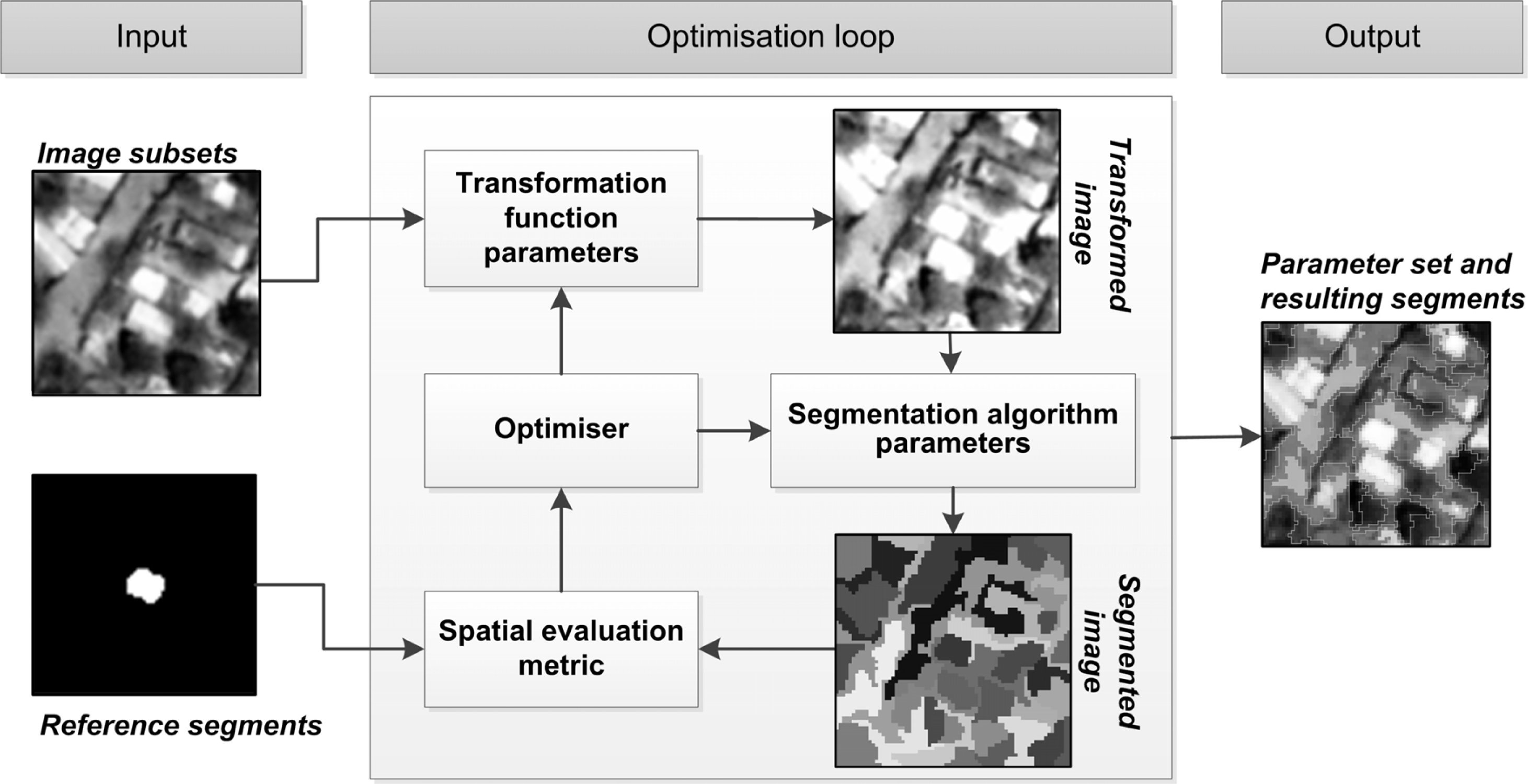
The method described here follows the general architecture of empirical discrepancy metric guided optimization-based methods [14,25,26]. Figure 1 illustrates the architecture of the variant presented in this work. The main contribution lies in the introduction of low-level image processing in the optimization loop, increasing the dimensionality of the search space. The method can be broken down into three distinct components. A user input component, the optimization loop, which constitutes the main body of the method and the output component.
The input component requires a user to provide input imagery and a selection of reference segments representative of the elements of interest. In our implementation such input data are handled separately with the reference segments delineated in a binary raster image, although sharing the metadata of the input image. As a preprocessing step, subsets are extracted from the input image and reference segments image over the areas where reference segments are provided. In Figure 1, such an image subset and corresponding reference segment subset is illustrated under the input component. It should be noted that the method takes as input all created subsets (a subset stack), not just those of a single element as depicted in Figure 1 for simplicity. The collection of input image and reference segments subsets are used within the optimization loop.
The optimization loop consists of an efficient search method traversing two parameter domains simultaneously and receiving feedback from a spatial metric (empirical discrepancy method). The search method used here is detailed in Section 2.2. Figure 1 illustrates the interacting processes at iterations of the optimization loop. Firstly a parameter set is transferred from the optimizer to a given data transformation function (low-level image processing process). This data transformation function, with the provided parameter values, is invoked on the input image subsets returning transformed image subsets. A range of low-level image transformation functions are tested with this method, detailed in Section 2.3.
A second parameter set is passed on from the optimizer to the given segmentation algorithm. The segmentation algorithm with its provided parameter values is invoked on the transformed image subsets, resulting in a stack of segmented images (as in Figure 1). The segmentation algorithms used in this work are detailed in Section 2.4. Finally a spatial evaluation metric is invoked, taking as input the reference segments subsets (under “input”) and the segmented image subsets. The final score given by the evaluation metric is the average over all provided reference segment subset and segmented image subset pairs. In the context of using metaheuristics such a metric is also referred to as an objective or fitness function. This score is passed on to the optimizer, which uses the information to direct the search in the next iteration. A range of single-objective evaluation metrics are tested in this work, detailed in Section 2.5. In Section 2.6 some example segmentation results are highlighted, with different parameters from the segmentation algorithm and data transformation domains and accompanying metric scores.
The method terminates after a certain number of user defined search iterations have passed, but various other stopping strategies are possible. As an output the parameter set resulting in the best segmentations are given, as judged by the evaluation metric. Note that during the search process processing is only done on the small image subsets to reduce computing time. After the method terminates the output (parameter set) can be used to segment the whole image or other images. Cross-validation and averaging strategies may help to ensure generalizability.
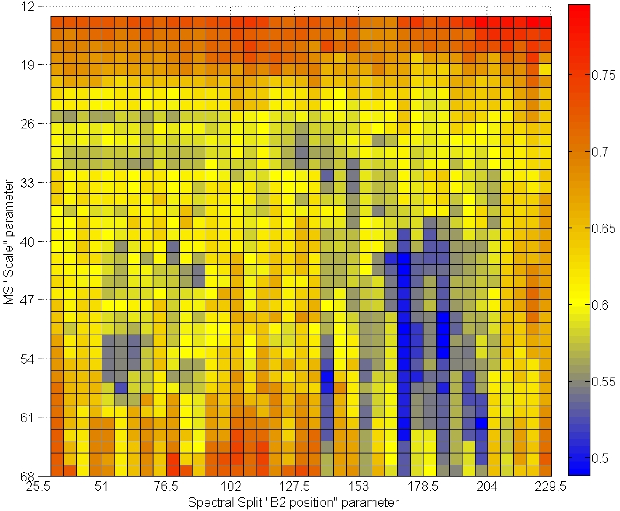
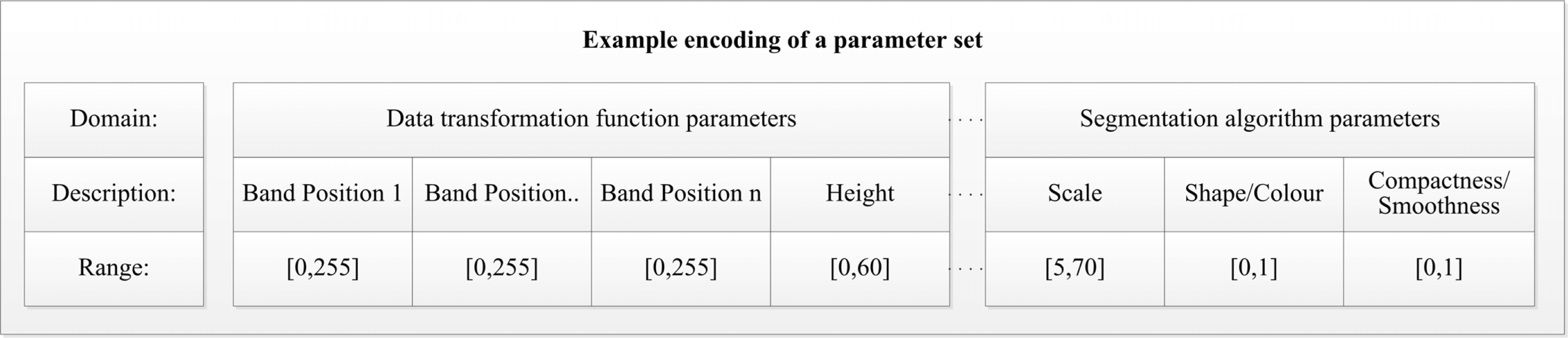
Figure 2 illustrates an example encoding or parameter space that is traversed by the search algorithm. In this example the parameter space consists of a four parameter data transformation function (Spectral Split, detailed in Section 2.3) and a three parameter segmentation algorithm (Multiresolution Segmentation (MS), detailed in Section 2.4) resulting in a combined seven dimensional search space. The value ranges of the parameters are also shown. In our implementation all quantizations for parameters are converted to real values, due to the use of a real-valued optimizer. Figure 3 illustrates a two-dimensional exhaustive calculation of fitness of the seven dimensional parameter space from Figure 2 on an arbitrary problem and metric, highlighting multimodalities or interdependencies between two parameters from the two different parameter domains. Lower values suggest better segmentation results.
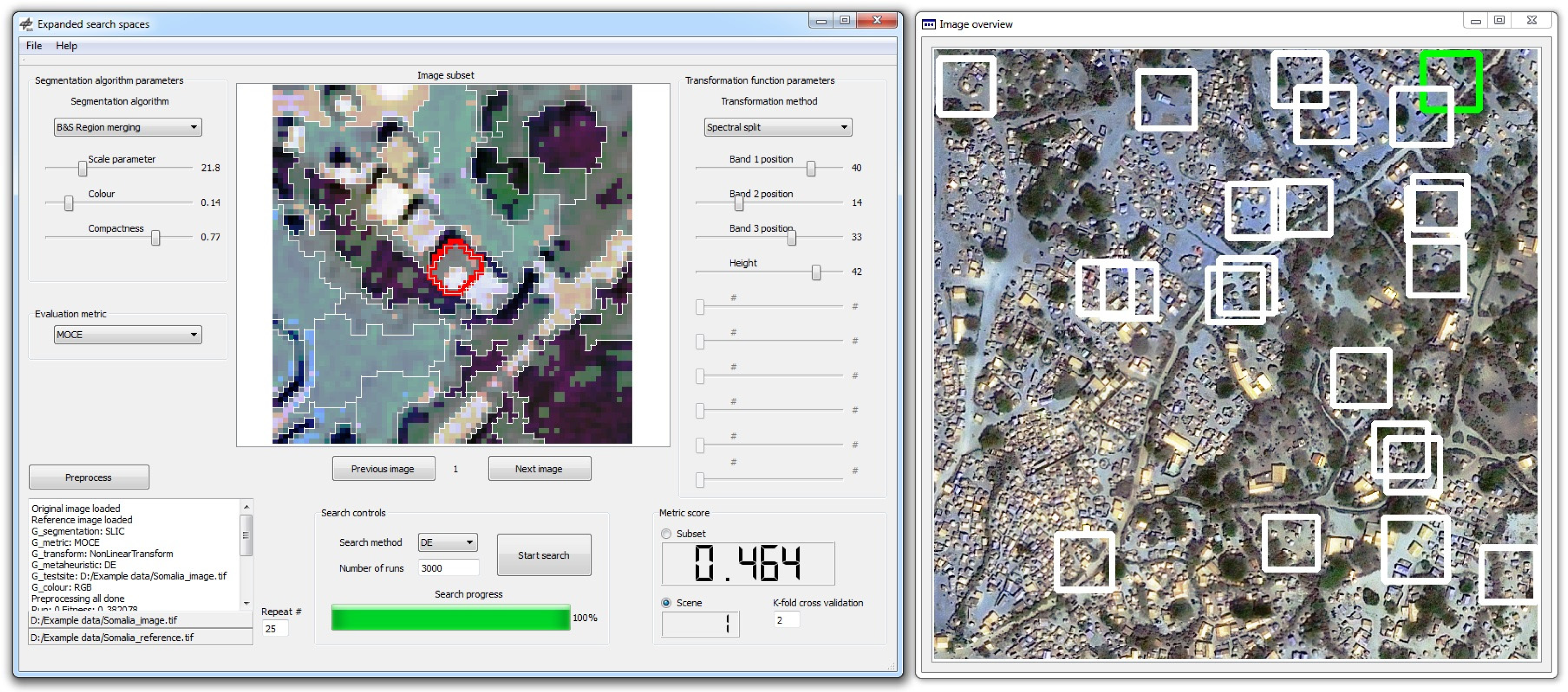
In practice such a method could be implemented as a user driven software application or add-on, as illustrated in Figure 4. A user could be given the ability to digitize or select reference segments as well as control the search process and assess the results in a quantitative and qualitative manner. Intervention in the parameter tuning process of the segmentation algorithm and the data transformation function could be facilitated with user input controls, for example via interactive parameter sliders to visualize changes in segment results. Thus the method could function in a manual or automatic manner. Such a tool or method could be used independently or as part of a more encompassing image analysis process.
2.2. Differential Evolution Metaheuristic
Due to the potentially complex search landscapes (e.g., Figure 3) generated by the parameterized algorithms and evaluation metrics, stochastic population-based search methods are commonly employed in sample supervised segment generation approaches [14,26,30]. Such search methods do not use any derivative information (gradients) from the search landscape to direct the search. These methods have multiple agents or individuals traversing the search landscape, with information exchange among the agents and individual behavior controlling the convergence and exploration characteristics of aforesaid methods.
The Differential Evolution (DE) metaheuristic is used here, specifically the “DE/rand/1/bin” variant detailed in [53]. DE generalizes well over a range of problems, is intuitive and relatively easy to implement. For experimental conformity the population size is kept constant at 30 agents (random starting positions), although the search landscape dimensionalities range from two to thirteen. See [53] for details on the formulation of DE. The amplification factor of the difference agent (F) is set to 0.75 and the crossover constant (CR) to 0.3. DE was chosen and tuned based on preliminary experimentation [18] comparing it with other simple metaheuristics (particle swarm optimization, modified cuckoo search) for typical problem types addressed here, also corroborated with findings elsewhere [30,54].
2.3. Data Transformation Functions
In image processing simple data transformation or mapping functions are typically employed for image enhancement, implying an image is changed for either easier interpretation or for easier/more accurate further processing. Functions are typically point- or neighborhood-based, taking as input pixel values and giving as output new values. Point-based functions modify values taking as input only data from the given pixel (e.g., contrast stretch). Neighborhood-based functions also use data from surrounding pixels to modify a pixel (e.g., smoothing and edge-detection filters). Transformation functions may have controlling parameters influencing the output. In this work four transformation functions possessing controlling parameters are tested. All input imagery is assumed to consist of three bands.
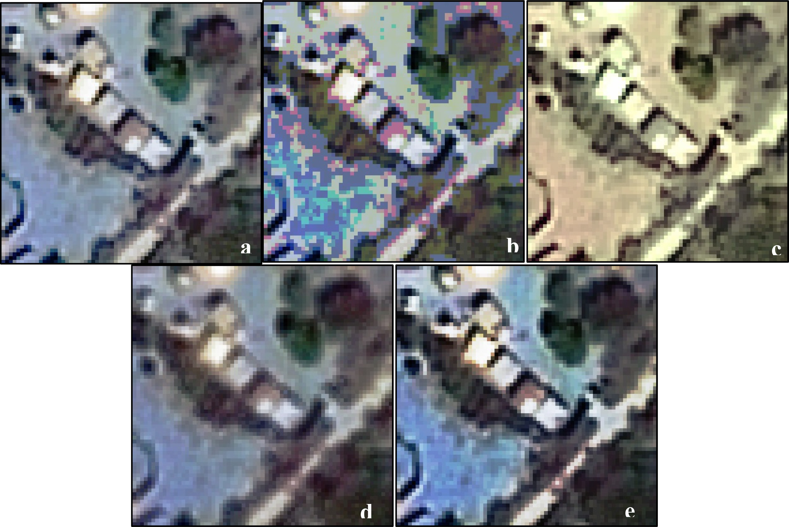
Figure 5 illustrates an unmodified subset of a satellite image depicting small structures (Figure 5a), along with four transformation functions (Figure 5b–e) investigated in this work. Controlling parameters were given random values in generating the figures. The transformation functions vary in terms of observing local and neighborhood properties, observing multiple bands, algorithm flexibility and number of parameters. The four transformation functions are briefly described.
2.3.1. Spectral Split
Spectral Split [52] is a simple n + 1 parameter transformation function where n is the number of bands in the image. The transformation function changes the values of pixels around a specified, parameterized value called position. For each band (n) of the input image, there is a corresponding position parameter. Another parameter, called height, controls the magnitude of the change around the position parameter(s). Pixels outside the range height compared to position are unaffected by the transformation. Spectral Split can be written as:
2.3.2. Transformation Matrix
A transformation matrix is tested here as a data transformation function (entitled Transformation Matrix), commonly used for color space transformations. Pixels of a given coordinate of an image stack can be represented as a point matrix. Multiplying the point matrix with a transformation matrix gives as output a new transformed point matrix. In the case of three image bands, such a transformation matrix consists of nine variables, modelled here as parameters for an image transformation (Equation (2)). Such a transformation allows certain bands to carry more weight, or highlight certain synergies of the data (see Figure 5c). The range of the parameters is set to [−0.2, 1]. As opposed to the other transforms described here, which only consider pixel values, spatial aspects and parameter values, the Transformation Matrix allows for a change of pixel values based on parameters and values from other channels.
2.3.3. Genetic Contrast
Some works also propose to consider image contrast enhancement as a parameterized optimization problem, with a variant considering local spectral distributions proposed in [48,55]. A real valued encoding variant [55] of this image enhancement method is tested as a low-level transform, entitled Genetic Contrast for convenience. Genetic Contrast changes a pixel’s value based on global image spectral characteristics, local characteristics (neighborhood standard deviation and mean values) and four controlling parameters (see Figure 5d). Genetic Contrast is written as:
With G denoting the image global mean value, σ(x) the standard deviation around pixel x and m(x) the mean around pixel x. Controlling parameters are denoted with a, b, c, and k, with ranges [0, 1.5] for a, [0, G/2] for b, [0, 1] for c, and [0.5, 1.5] for k.
2.3.4. Genetic Transform
General approaches have also been put forth that consider low-level image processing as an optimization problem, with some of the early works focussing on basic image enhancement [49,56]. Such an approach is investigated here as a potential low-level transform forming part of the combined low- and mid-level image processing search landscape. A ten parameter transformation function [49,56], for convenience called Genetic Transform, is tested. Genetic Transform consists of four parameter-controlled non-linear transformation functions, with either one or two controlling parameters. These four functions are weighted (convex combination) by four additional parameters to form a singular function. This allows for flexibility in the prominence of the different transforms, in addition to flexibility in the actual structures of the mappings. All bands in an image are handled with the same functions (parameters). Input values are scaled to the range [0, 1]. The four transforms are written as Equations (4–7).
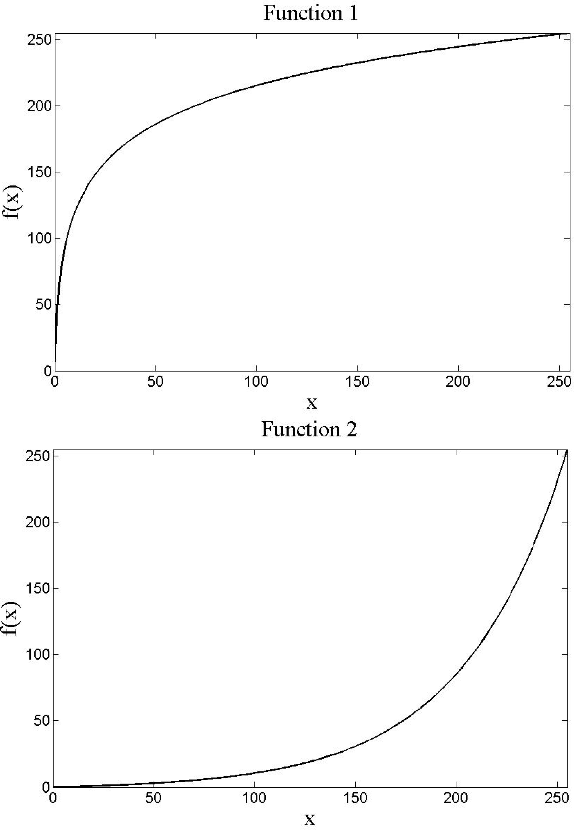
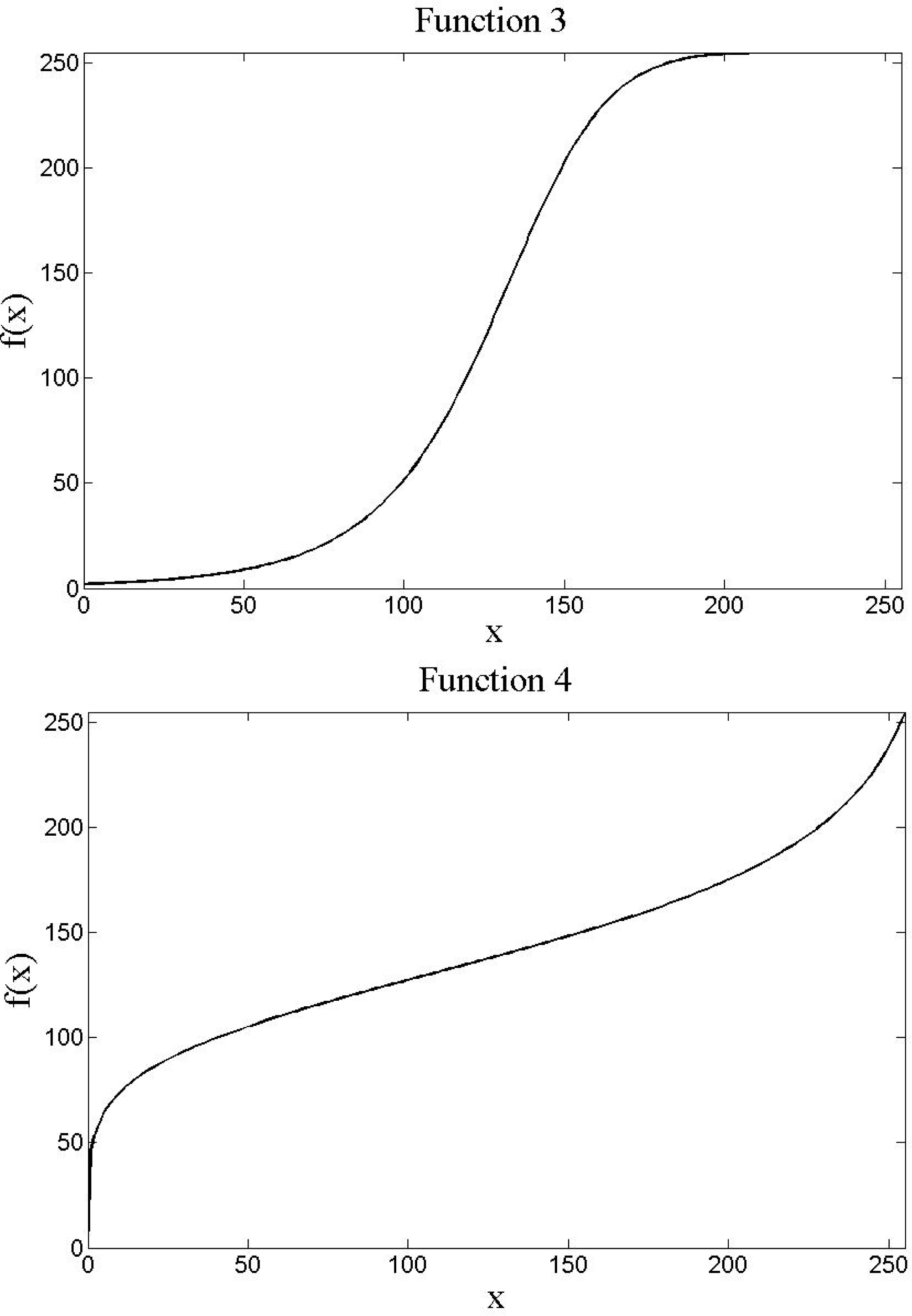
Figure 6 illustrates example mappings of the four functions with arbitrarily chosen parameter values. The combined function is written as:
Similar to Spectral Split, Genetic Transform is a point-based function that could lead to stronger spectral discontinuities or continuities due to the non-linear rescaling of the data (Figure 5e). In contrast, it has more controlling parameters, increasing search landscape dimensionality, but is theoretically more flexible and may, thus, fit better to a given problem.
2.4. Image Segmentation Algorithms
Two image segmentation algorithms are tested within the approach described, a fast clustering algorithm and a variant of region-merging segmentation.
2.4.1. Simple Linear Iterative Clustering Algorithm
Simple Linear Iterative Clustering (SLIC) [57] is considered a superpixel algorithm—which attempts to group an image into larger spectral atomic units as opposed to the original pixel level. The algorithm is intended for use on natural color imagery. Semantic segmentation is typically not attempted with such algorithms, but results may be used in further segmentation processes. The SLIC algorithm clusters (segments) pixels in a five dimensional space using region constrained k-means clustering. The space consists of the two dimensions of the image (x and y dimensions) and three input bands; which are assumed to be in the red, green, blue color space. The SLIC algorithm converts the RGB color space to the CIELAB color space before further processing (not done in this work). SLIC is used here with some liberty in the context of semantic image segmentation due to the computational efficiency of the algorithm, allowing for near real time manual segmentation algorithm parameter tuning, and middling segmentation results on problems addressed in this work.
2.4.2. Multiresolution Segmentation
The basic Multiresolution Segmentation (MS) algorithm [10] is a three parameter variant of region-merging segmentation. The scale parameter of the MS algorithm, which incorporates notions of the spectral degree of fitting before and after a virtual segment merge and object size, controls the relative sizes of segments. Two other parameters namely shape/color and compactness/smoothness controls the weight of two geometry homogeneity criteria (compactness and smoothness [10]) against each other (compactness/smoothness) and against the scale parameter (shape/color). Other geometric homogeneity criteria may also be considered [29]. A variant not considering band weighting [10] is utilized.
2.5. Spatial Metrics
Four empirical discrepancy metrics are employed as fitness functions to direct the search process. These four fitness functions are utilized in the context of single-objective optimization and use notions of spatial overlap, as opposed to edge matching or empirical goodness metrics. Doing comparative experimentation with multiple fitness functions are advocated (four in our case), as quality are measured differently among the functions. Various metrics matching a single generated segment to a reference segment have been shown to be highly correlated [15], with a singular metric in the test bed considering over- and under segmentation more elaborately diverging from the correlation [15]. Thus, results are reported with a metric matching a single generated segment to that of a reference segment and three metrics allowing for multiple generated segments to be matched with a given reference segment (having internal differences). Metrics allowing for multiple generated segments to be matched with a single reference segment are more flexible to a wide range of problem instances, for example if some reference segments are routinely over-segmented or if, due to segmentation algorithm limitations, over-segmentation is common.
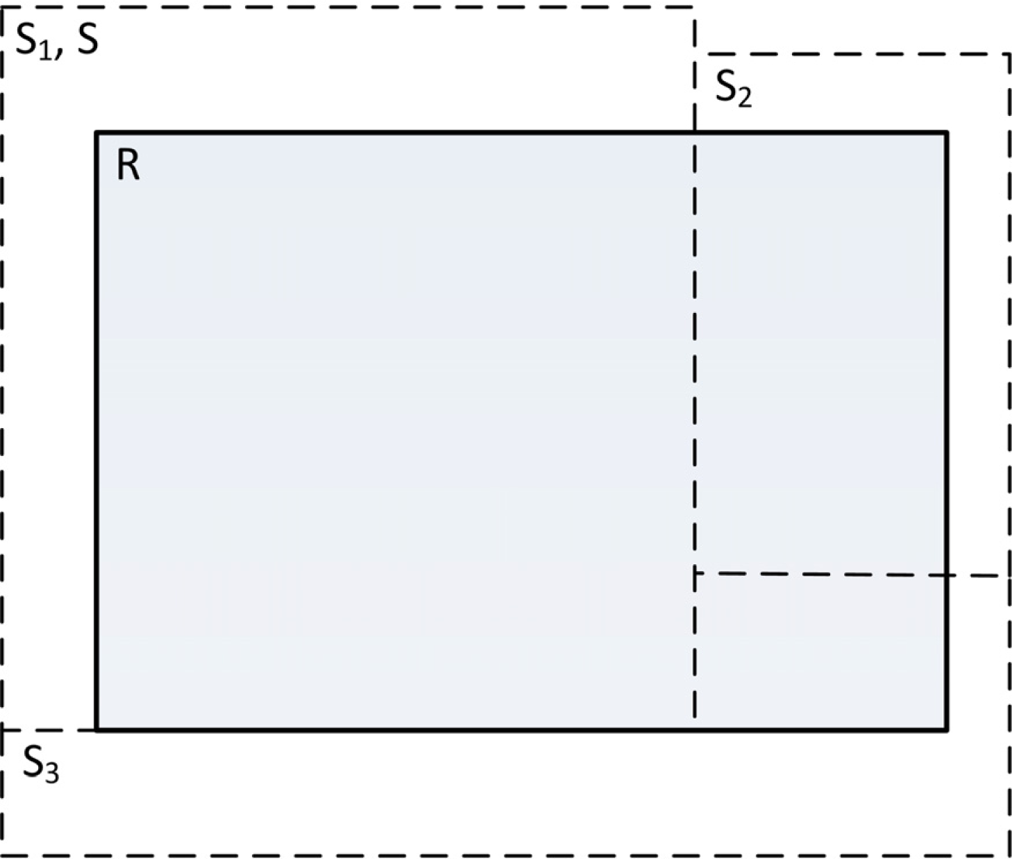
Figure 7 illustrates an abstract segmentation evaluation scenario with the reference segment denoted by R, generated segments intersecting the reference segment by Si, the generated segment with the largest overlap with the reference segment as S and the number of segments intersecting with R as n. Results of such evaluations are averaged over multiple reference segments. The four utilized metrics are described using set theory notation. “| |” Denotes the cardinality (the number of pixels in the segment). The optimal value for all metrics described here is zero.
2.5.1. Reference Bounded Segments Booster
The Reference Bounded Segments Booster (RBSB) [25] metric measures the amount of mismatch between R and S against R, with a range of [0, ∞] and can be written as:
2.5.2. Larger Segments Booster
A variant of the Larger Segments Booster (LSB) [31] metric is used here, written as:
2.5.3. Partial and Directed Object-Level Consistency Error
Inspired by the Object-level Consistency Error (OCE) [17], which is influenced by the Jaccard index [58], a partial and directed variant of OCE is defined, entitled PD_OCE, with a range of [0, 1] and written as:
A specific Si covering only a fraction of R but with a very large component outside of R have a large influence on the metric score, which could be an erroneous quality notion in many problem instances.
2.5.4. Reference Weighted Jaccard
Also inspired by the Jaccard index, a new metric is proposed, the Reference Weighted Jaccard (RWJ), with a range of [0, 1] and written as:
As opposed to the OCE/PD_OCE metric, the RWJ metric weights the summation of results against the contribution of Si to R.
2.6. Examples of Data Transforms with Segments and Metric Scores
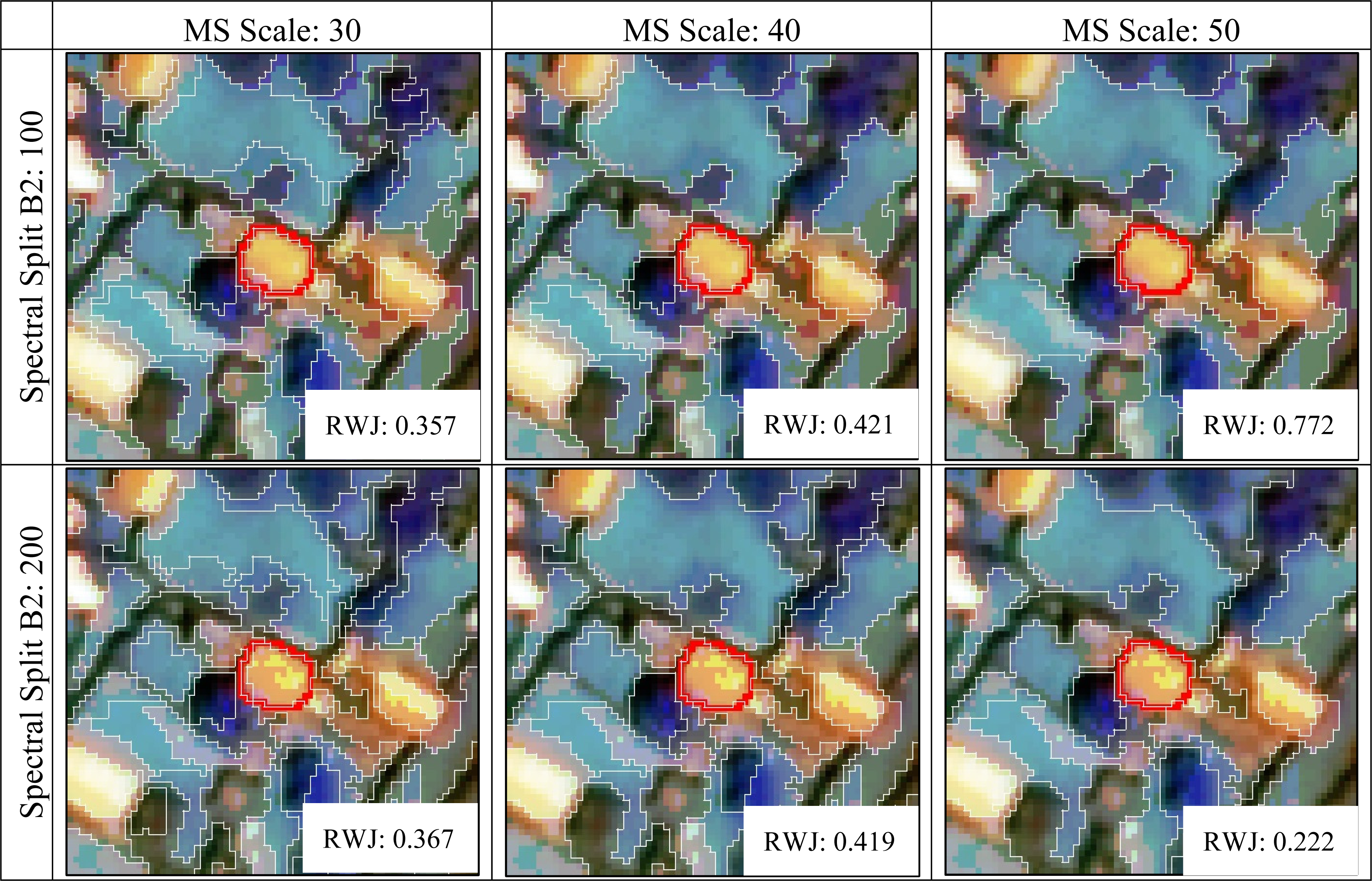
Figure 8 illustrates several different combinations of data transformation function parameters (Spectral Split) and segmentation algorithm parameters (Multiresolution Segmentation) in terms of RWJ metric scores. The other parameters of the segmentation algorithm and transformation function were kept constant. Note the differences in metric scores when considering a MS scale parameter of 50.
3. Data
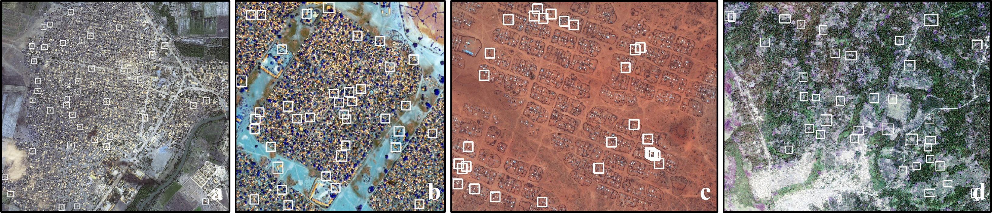
Four example problems are addressed and tested with this approach. Fully pre-processed subsets of VHR optical imagery (Figure 9) were obtained, depicting a settlement (Jowhaar, Figure 9a), refugee camps (Hagadera, Bokolmanyo, Figure 9b,c) and a settlement surrounded by informal agriculture (Akonolinga, Figure 9d). The aims could be to obtain information for conducting urban planning (Figure 9a), structure counting and characterization (Figure 9b,c) and agricultural monitoring for land-use planning (Figure 9d). It is attempted to segment structures (Figure 9a–c) and fields (Figure 9d) using a single segmentation layer using the sample supervised segment generation approach described. Provided reference segments are enclosed by white bounding boxes. The Bokolmanyo site (Figure 9c) pose an easy segmentation problem, with the other three problems proving to be more difficult to segment accurately using only a single segment layer. In practice subsequent processes could refine results, especially on the more difficult problems. All imagery consists of three input bands, have 8-bit quantization and are pansharped. Table 1 lists some image metadata, including the number of utilized reference objects or segments for each image.
4. Methodology
The method described here is quantitatively compared in terms of segmentation accuracies with a general sample supervised segment generation approach not performing any data transformations (detailed in Section 4.1). Several search methods are investigated with such an approach, to validate the usefulness of more complex variants (Section 4.2). In addition to the segmentation evaluation, some convergence profiling is done on variants of the method. Finally the presences of parameter interdependencies are investigated to justify the creation of enlarged search spaces (Section 4.3).
4.1. Data Transformation Functions for Expanded Search Spaces
The general usefulness of transformation function expanded search spaces is investigated. The four sites and reference segments detailed in Section 3 (Figure 9) is used with the sample supervised segment generation approach detailed in Section 2. For each site, the method is executed using the four transforms described in Section 2.3 and using the MS and SLIC segmentation algorithms. In addition to using the transforms, the method is also run using no data transformation function. Evaluation is conducted using the four different evaluation metrics described in Section 2.5. In total, 40 different experimental setups or methodological variants are tested per site, allowing for evaluating the usefulness of such an approach in general, but also giving indicators of the usefulness of specific transforms and segmentation algorithms.
The utilized DE metaheuristic is given 3000 search iterations (30 agents) to traverse the search space in all experimental instances, thus, not giving enlarged search spaces more computing time or evaluations. All experiments are repeated 25 times to generate a measure of specificity and also to allow for testing the statistical significance among method variants, amounting to ± 250 million segmentation evaluations. Two-fold (hold-out) cross-validation is performed in all experimental runs to prevent overfitting of the parameter sets to the given reference segments.
4.2. Metaheuristic Evaluation and Convergence Behavior Profiling
The appropriateness of using a population based metaheuristic on the search spaces created by combining simple transformation function parameters and segmentation algorithm parameters is investigated. For two of the test sites, the proposed method is run using four different transformation function strategies. The DE metaheuristic is compared for such applications (search landscapes) with simple to implement search strategies, namely a Hill Climber (HC) and Random Search (RND). For each test site, using the different transformation function strategies, the three search methods are compared via fitness trace characteristics and resultant segment quality after 3000 search iterations. Fitness traces/plots are averaged over 25 runs.
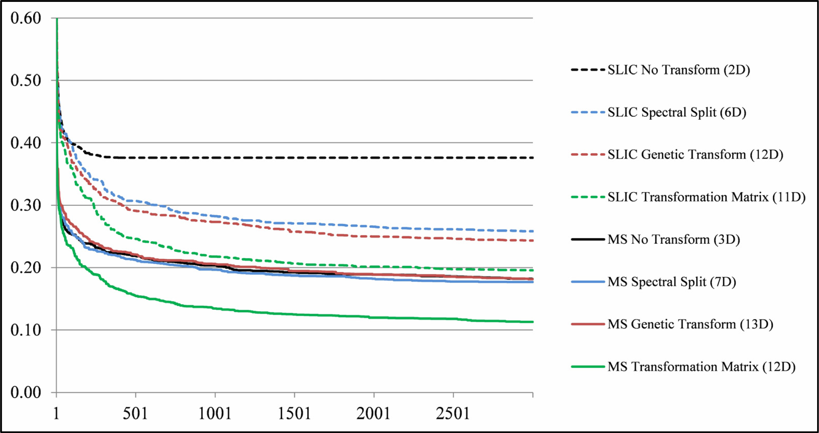
The convergence behavior of the method operating under no data transformation and data transformation conditions is also investigated. Four of the transformation strategies are compared. Due to the computationally expensive nature of such an approach, a search process should typically be terminated as soon as possible. It is investigated how larger search space variants compare with simpler, lower dimensional, variants in terms of convergence behavior, for example to determine if simpler variants have some early accuracy advantage over complex variants.
4.3. Parameter Domain Interdependencies
As with classification, search processes can suffer from the curse of dimensionality. Problems could be decomposed into smaller separate problems for more efficient processing if there exist no interdependencies [50,51] among the processes or parameter domains. Some processes could add value to a solution without, or minimally, interacting with other processes. In the context of GEOBIA, examples could be post hierarchical segmentation segment merging procedures observing attribute criteria, contextual classification not sensitive to segment characteristics (segmentation algorithm parameters) or a form of spectral transformation and segmentation (e.g., mathematical morphology) resulting in slightly different/better segments, as opposed to not performing the spectral transformation, but having identical segmentation algorithm parameters.
Tests are conducted to validate the existence of interdependencies between the data transformation function parameters and segmentation algorithm parameters used in this study, which can be strongly anticipated in this context. The sample supervised method described here is run on a test site using the two segmentation algorithms, four metrics and four transforms in selected combinations. The optimal segmentation algorithm parameter values generated by the variants of the method are recorded (25 runs) and contrasted, specifically the differences when using different transforms versus using no transformation function. Differing optimal values gives an indication of interdependencies.
Furthermore a simple statistical variable interdependency test is performed between parameters from the segmentation algorithm and data transformation function domains, as detailed in [50]. A variable or parameter xi is affected by xj if, given a parameter set a =(…, xi,…, xj,…) and b =(…, x′i, …, xj,…) and f(a) ≤ f(b) (fitness evaluation), with a change of xi to x′j in sets a and b to create a′ and b′, the equation f(a′) > f (b′) holds. For one site, using the MS segmentation algorithm and Spectral Split transformation function, an exhaustive parameter dependency test based on 100 randomly initiated values for the described evaluation is performed. Any value above 0 indicates variable interaction, although higher values suggest more regular interaction.
5. Results and Discussion
5.1. Data Transformation Functions for Expanded Search Spaces
Tables 2 and 5 list the results of the experimental runs on the four test sites. The values indicate the best fitness achieved, averaged over 25 runs. The standard deviations are also given. Different data transformation functions may be contrasted within each metric category (horizontal grouping). Lower values indicate better results. Results from different metrics cannot be compared (vertical grouping), although the results from the two segmentation algorithms within each metric category may be contrasted. The shaded cells delineate results obtained using variants of the method employing data transformations that resulted in worse quality scores compared to the variant of the method using no data transformations. Results that are not statistically significantly different from the no transformation variant according to the student’s t-test with a 95% confidence interval are also delineated with shaded cells.
Examining Tables 2 and 5 it is evident that simple expanded search spaces (under identical search conditions) can assist in generating better quality segments. The magnitude of the improvement depends on the definition of quality (metric), the characteristics of the features of interest in the image as well as the specific data transformation function employed. Notwithstanding, under certain metric and transformation function conditions, consistently worse results are obtained. The Genetic Contrast transformation function in particular does not add value to most problem instances investigated here. This could be due to the smoothing/distorting effect of the function (Figure 5d). In addition, the Spectral Split function only improves results fractionally, if at all.
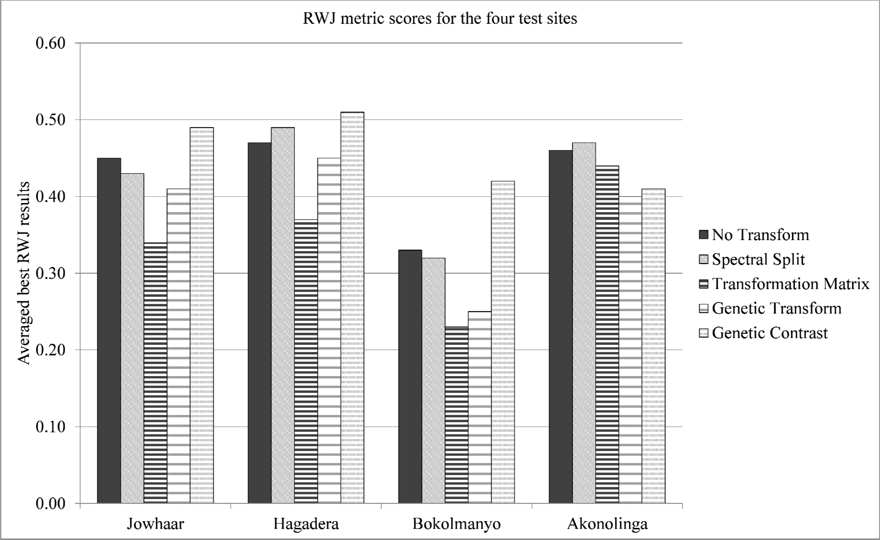
Adding the Transformation Matrix and Genetic Transform functions on the other hand almost always results in improved segmentation accuracies, with varying magnitudes. Figure 10 highlights RWJ metric scores using SLIC as the segmentation algorithm. Note the performances of the Transformation Matrix and Genetic Transform functions. Under a few metric and image conditions (Tables 2 and 5), improvements in excess of a decrease of 0.20 in metric values are noted with these two transforms. In the eight instances where these functions did not improve results, the results were not worse by more than a 0.02 change in metric values (minor) and only requiring neglectable additional computing for performing the data transformation.
The behavior of the RBSB metric on the Akonolinga site using the SLIC segmentation algorithm could be due to the fact that the given range of the scale parameter in SLIC was not sufficiently large to segment some of the relatively large fields in this scene. RBSB matches the largest overlapping generated segment with the reference segment, potentially creating noise/discontinuities in these instances and thus causing difficulty for the search algorithm (30 randomly initialized agents).
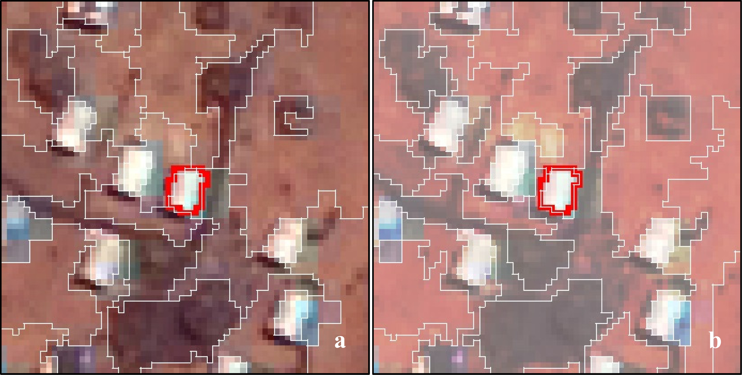
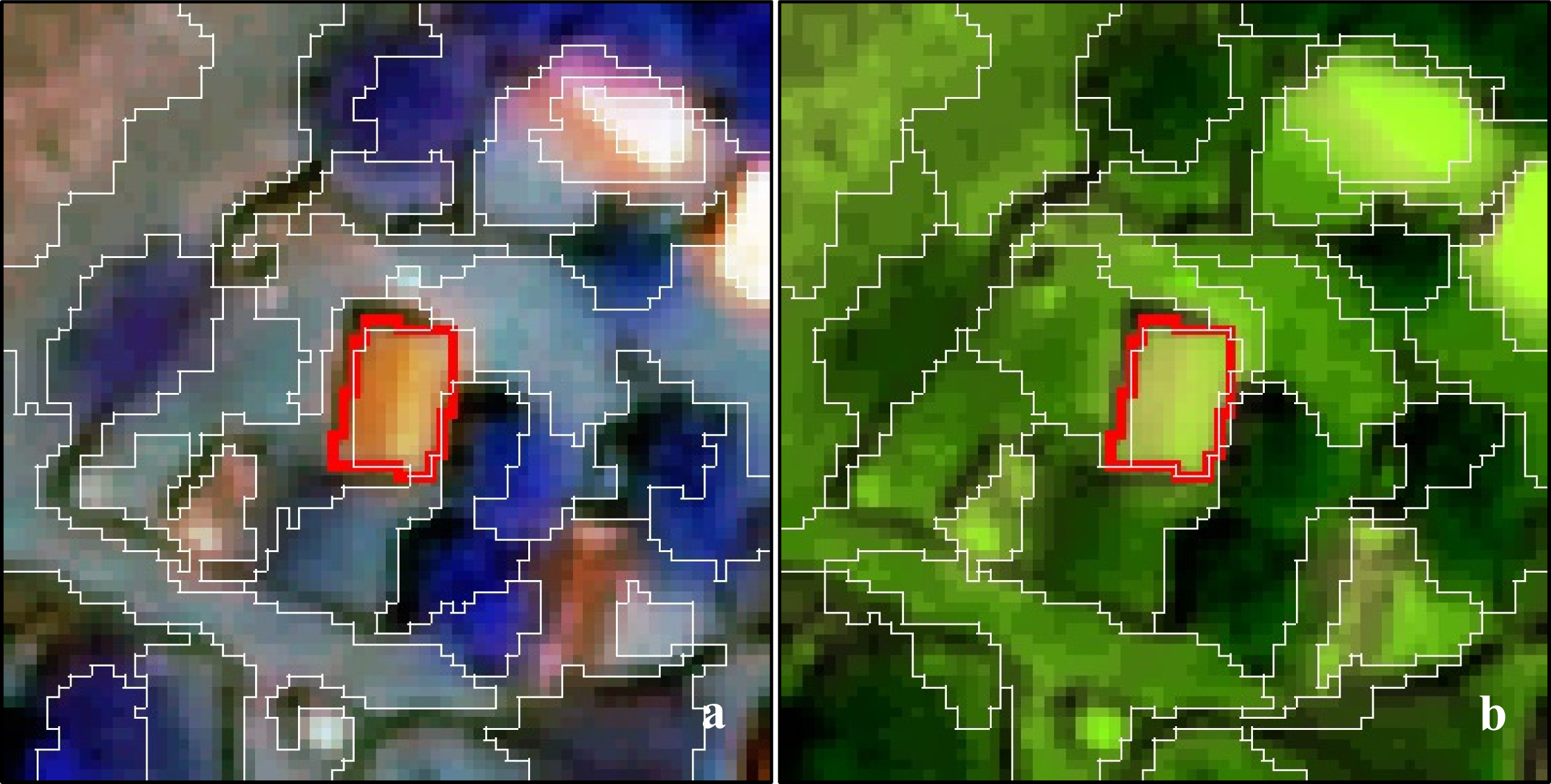
Figures 11 and 12 highlight the best segmentations achieved with different transformation functions compared to the variant of the method not performing transformations. Note the more accurate boundaries on the reference segments (outlined in red) as well as better fits on structures not delineated due to averaging results and performing cross-validation to improve generalizability. Additional post-segmentation processing steps could improve results. In addition, note that image transformation is done solely for the purpose of generating better segments. Subsequent processes/methods should run on the original image data (e.g., Figure 11a), but using the segments generated on the transformed space (e.g., Figure 11b).
5.2. Metaheuristic Evaluation and Convergence Behavior Profiling
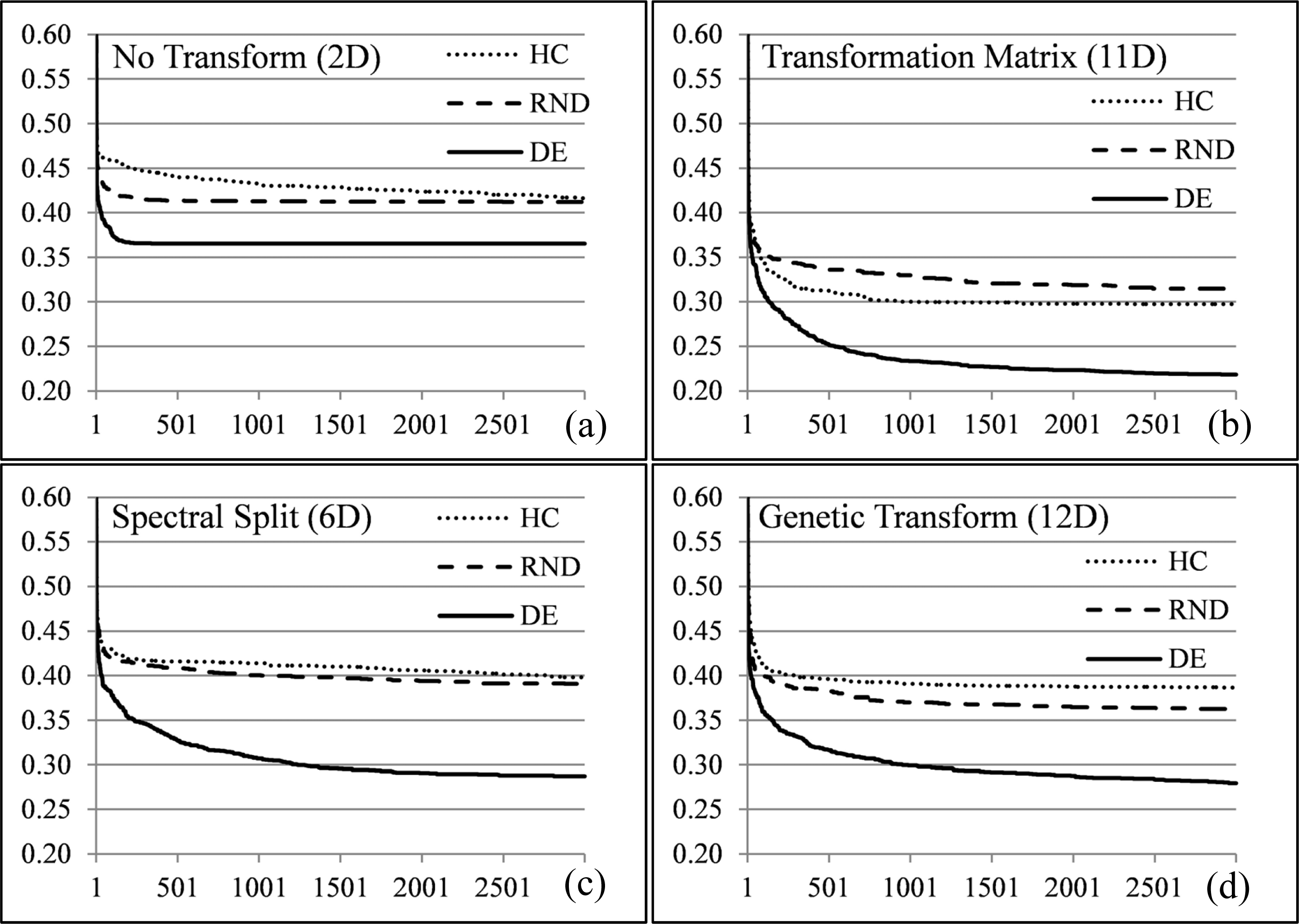
Figures 13 and 14 illustrate the fitness traces of the DE, HC and RND search methods averaged over 25 runs for the elements of interest (averaged) in the Bokolmanyo and Jowhaar sites. Each sub-graph illustrates results using a different image transformation strategy. The search landscape dimensionalities of the different method variants are given in brackets. Final metric scores may differ from results presented in Section 5.1 due to cross-validation, which is not possible here for a fitness trace.
In all instances the differential evolution method gave the best final metric scores as well as maintaining the lowest values during the search process. This highlights some difficulty (discontinuities/ruggedness, deceptiveness, and multimodality) of the search landscapes (e.g., Figure 3), necessitating the use of more complex search strategies. Within a few generations, less than 250 search iterations, the DE search strategy starts to deliver meaningfully better results compared to the other two simple search strategies. As the dimensionality of the problem increases, in general, the magnitude of the differences in the results of the DE versus HC/RND increases. The advantages of using a more complex search strategy like DE is much more marginal when considering the variant of the method not employing any data transformation (Figures 13a and 14a).
Figure 15 shows fitness traces generated for the Jowhaar site using the SLIC and MS segmentation algorithms and four of the transformation function strategies. It is evident that simpler, or lower dimensional strategies (e.g., No Transform or Spectral Split) do not provide an initial performance increase over more complex, higher dimensional, variants (e.g., Transformation Matrix and Genetic Transform). This could be due to general usefulness of some transforms leading to better results by just randomly selecting points in the search space, with the magnitude in fitness differences increasing as the actual search progresses. Different fitness traces rarely cross, with the Transformation Matrix strategy, for both SLIC and MS, providing better final metric scores as well as maintaining the best results throughout the search process. Considering the MS segmentation algorithm, the No Transform, Spectral Split and Genetic Transform strategies have very similar fitness traces, but with no penalty for using the more complex variants.
Interestingly for this specific problem, the MS algorithm outperforms the SLIC algorithm under any transformation condition. Additionally, observing the fitness traces in this section, it could be argued that 1000 to 1500 search iterations are sufficient, keeping in mind the problems, metrics and transformation functions considered.
5.3. Parameter Domain Interdependencies
Tables 6 and 7 lists the parameters obtained for the MS and SLIC segmentation algorithms under different metric and data transformation conditions. The achieved fitness scores are also given. Examining Table 6, which denotes resultant parameters with the MS algorithm, very specific final fitness scores (low standard deviations) are generated by a wide range of different parameter sets under each data transformation condition. Thus multiple optima exist when considering the MS algorithm that approximates to the same (optimal) achievable segmentation quality, similar to the blue shaded cells illustrated for an arbitrary problem in Figure 3. None the less, various combinations of optimal scale parameter values achieved under different transformation conditions are statistically significantly different according to the student’s t-test with a 95% confidence interval (e.g., MS/PD_OCE No Transform and Spectral Split), suggesting different optimal values under different transformation conditions.
Table 8 lists the achieved scale parameter values over the allocated 25 runs using the RWJ metric and no data transformation as shown in Table 6. Note the two distinct value ranges, around 7–9 and again at 24, resulting in the high standard deviation of 17.66 for the scale parameter, but still resulting in a fitness score with a standard deviation of less than 0.02. Under all transformation conditions, low shape/color parameters are generated, with relatively low standard deviations. No significant conclusion can be made on the behavior of the shape/color and compactness/smoothness parameters.
Opposed to the results from the MS segmentation algorithm, the SLIC algorithm (Table 7) displays more specific scale and compactness parameter values as well as delivering very specific fitness scores. Again, various combinations of optimal scale parameter values achieved are statistically significantly different according to the student’s t-test with a 95% confidence interval. This verifies, as with the MS algorithm, apparent parameter dependencies between the parameter domains of the segmentation algorithms and data transformation functions.
Finally Table 9 lists the results of the parameter interdependency test [50] performed on the Bokolmanyo site with the MS algorithm and Spectral Split combination under the RWJ metric condition. The parameters listed on the vertical axis are considered affected by the parameters listed horizontally if the result of an interdependency test is greater than zero. The table is divided into four quadrants, depicting the interactions of the two parameter domains. If both the top right and bottom left quadrants returned 0 for all cells, the two parameter domains can be considered as not interacting. In this simple example, all parameters are affected by all other parameters, to varying degrees. This suggests interdependencies. Interestingly, considering 100 evaluations for each cell, some interdependencies are frequent or strong (of no importance in determining interdependency). The scale parameter of the MS algorithm can be considered as its most important or sensitive parameter, reflected by the high degree by which its value is affected by all the other parameters. Note that these results reflect parameter interactions or the frequency of interactions, and not the contributions to segment quality of the interactions.
6. Conclusions
6.1. Potential of Expanded Search Spaces in Sample Supervised Segment Generation
In this work a sample supervised segment generation method was presented and profiled. Expanded search spaces were introduced in the optimization loop, here by adding low-level image processing functions. In the context of segmentation problems, such an expanded search landscape allows for creating closer correlations between thematic and spectral similarity, allowing the given segmentation algorithms to generate better quality segments. In addition, such an extension to an automatic segmentation algorithm parameter tuning system is simple to implement.
An interesting and sometimes advocated effect of such sample supervised optimization based approaches, is their potential to generate good or quality solutions in ways an expert user might never have foreseen. In our examples the results from Table 7 (also see Figure 12b) serve as a good example of such a scenario. Combining the MS segmentation algorithm with the Transformation Matrix, setting a low scale parameter (compared to the other variants) and creating washed-out monotone imagery works very well in numerous problem instances.
Four parameterized data transformation functions, having varied and sometimes complex internal characteristics have been tested with this method. Experimentation was conducted under various problem, metric, transformation function and segmentation algorithm conditions with generally favorable results advocating the utility of this method compared to simpler variants. Generalizability was also considered, with numerous reference segments tested and all results given as cross-validated. Care should be taken in selecting combinations of segmentation algorithms and data transformation functions, as a worsening of results are also possible under certain conditions. Such transformation functions or modifications of the data are exclusively used internally in the segmentation process and the resulting transformed data have no use for further analyses or visualization procedures.
The utility of using more complex search methods for traversing these enlarged search spaces was also investigated. It was shown that simpler search strategies, such as a single agent hill climber and random search, were inefficient in exploring the search landscape compared to a differential evolution search strategy. In addition, variants of the method having much more parameters and thus significantly higher dimensional search spaces do not have any initial disadvantage in the search process compared to simpler variants or the variant not performing any data transformation. This suggests, in this context, no search duration penalty in adding transformation functions. Finally, it is shown via optimal achieved segmentation parameters and a simple interdependency test that the low-level and mid-level processes investigated here are (highly) interdependent, necessitating simultaneous optimization of these two parameter domains.
The method described here can be used on its own if the considered problem is simple enough, keeping in mind the capabilities of the segmentation algorithm. This could be judged by the output metric scores. A very low score implies results are sufficiently good to use the segments as is. Otherwise, such an approach could form part of a more complete image analysis strategy, where the method is used to generate intermediary results, with other methods or processes performing more encompassing image analysis. For example in an expert systems approach (e.g., rule set development) segments can be generated as optimally as possible, quantitatively judged, for a certain land-cover type before more elaborate processes are used to split, merge and classify segments.
6.2. Methodological Shortcomings and Open Questions for Future Research
Although such a method shows promise, some shortcomings and open issues are highlighted here. Firstly, the number of training samples needed by such a method to generalize well is unknown. In this work reference segment sets contained between 28 and 40 references, thus with two-fold cross-validation between 14 and 20 references were used to train the model. In preliminary experimentation, reference sets containing less than 5–8 references displayed bad generalization performance. More complex and thus more flexible models (search landscapes) might fit closer to the training reference segments than simpler variants and have worse generalizability, unless generalizability tests such as cross-validation are explicitly implemented.
Another open issue surrounding generalizability is how well different combinations of segmentation algorithms and low-level image processing generalizes over a range of problems, something not explicitly tested here. It could be stated that, considering the conditions in this study, the MS segmentation algorithm with the Genetic Transform and Transformation Matrix functions do perform well over a range of problems. Different low-level image processing functions might be suited to different problem types or categories. Future work could investigate additional promising functions used in combination with commonly used segmentation algorithms. Neighborhood based transforms might be worth investigating. Search landscape dimensionality should be kept in mind, as enlarged search spaces are more difficult to traverse.
The computationally expensive nature of image segmentation necessitates the efficient traversal of the search landscape. Such a sample supervised strategy advocates user interaction, so the method should ideally complete in a time frame acceptable to a user engaged with the image analysis. The computing time for a fitness evaluation iteration in this work (excluding Genetic Contrast) ranges from 0.10 ± 0.01 seconds (SLIC segmentation, 28 subsets from the Bokolmanyo site, No Transform) to 3.36 ± 0.28 seconds (MS segmentation, 40 subsets from the Akonolinga site, Genetic Transform) on an Intel Xeon E5-2643 3.5 GHz processor using single threaded processing. Running fitness evaluations (subset segmentation, transforms, fitness calculation) on a parallel computing architecture could be considered. In addition, motivated by the computationally expensive nature of fitness evaluation, more careful consideration could be given to the choice of the optimizer. Performing rigid meta-optimization (not conducted in this work), using metaheuristics with self-adapting metaparameters or hyperheuristics could be considered for further investigation.
The choice of an optimal metric is, in our opinion, an open issue. In this work four different metrics, which are able to measure over- and under-segmentation were used. In addition to the general “area-overlap” metrics tested here, metrics observing spectral characteristics and boundary offsets could be considered. Metrics sensitive to user inaccuracies in delineating reference segments could also be considered. It is still unclear how different metrics relate or correlate to final classification accuracies. Multi-objective optimization may also be considered.
Finally, the optimization concept of “epistatic links” (parameter interdependencies) [51] could, in some sense, be applied to some interactions in GEOBIA processes [8,9]. In this work an interaction between two domains was investigated and profiled. Investigating the potential of modelling classical GEOBIA processes as complex optimization problems could be profitable. Quality can be measured via empirical discrepancy methods, empirical goodness methods and even traditional notions of classifier accuracies.
Acknowledgments
This work has been conducted under the GIONET project funded by the European Commission, Marie Curie Programme, Initial Training Networks, Grant Agreement number PIT-GA-2010-264509. The programming libraries OpenCV, TerraLib and SwarmOps were used in this work.
Author Contributions
Christoff Fourie conceived the concept presented, implemented the methodologies, conducted the experimentation and wrote the manuscript. Elisabeth Schoepfer contributed to revision and editing.
Conflicts of Interest
The authors declare no conflict of interest.
References and Notes
- Addink, E.A.; van Coillie, F.M.B.; de Jong, S.M. Introduction to the GEOBIA 2010 special issue: From pixels to geographic objects in remote sensing image analysis. Int. J. Appl. Earth Observ. Geoinf 2012, 15, 1–6. [Google Scholar]
- Blaschke, T. Object based image analysis for remote sensing. ISPRS J. Photogramm. Remote Sens 2010, 65, 2–16. [Google Scholar]
- Hay, G.J.; Castilla, G. Geographic Object-Based Image Analysis (GEOBIA): A New Name for A New Discipline. In Object-Based Image Analysis: Spatial Concepts for Knowledge-Driven Remote Sensing Applications; Blaschke, T., Lang, S., Hay, G.J., Eds.; Springer: Berlin, Germany, 2008; pp. 75–90. [Google Scholar]
- Blaschke, T.; Hay, G.J.; Kelly, M.; Lang, S.; Hofmann, P.; Addink, E.; Feitosa, R.Q.; van der Meer, F.; van der Werff, H.; van Coillie, F.; et al. Geographic object-based image—Towards a new paradigm. ISPRS J. Photogramm. Remote Sens 2014, 87, 180–191. [Google Scholar]
- Atkinson, P.M.; Aplin, P. Spatial variation in land cover and choice of spatial resolution for remote sensing. Int. J. Remote Sens 2004, 25, 3687–3702. [Google Scholar]
- Hay, G.J.; Castilla, G.; Wulder, M.A.; Ruiz, J.R. An automated object-based approach for the multiscale image segmentation of forest scenes. Int. J. Appl. Earth Observ. Geoinfor 2005, 7, 339–359. [Google Scholar]
- Drǎguţ, L.; Tiede, D.; Levick, S.R. ESP: A tool to estimate scale parameter for multiresolution image segmentation of remotely sensed data. Int. J. Geogr. Inf. Sci 2010, 24, 859–871. [Google Scholar]
- Baatz, M.; Hoffman, C.; Willhauck, G. Progressing from Object-Based to Object-Oriented Image Analysis. In Object-Based Image Analysis: Spatial Concepts for Knowledge-Driven Remote Sensing Applications; Blaschke, T., Lang, S., Hay, G.J., Eds.; Springer: Berlin, Germany, 2008; pp. 29–42. [Google Scholar]
- Lübker, T.; Schaab, G. A work-flow design for large-area multilevel GEOBIA: Integrating statistical measures and expert knowledge. Int. Arch. Photogramm. Remote Sens. Spat. Inf. Sci 2010. Available online: http://www.isprs.org/proceedings/XXXVIII/4-C7/pdf/luebkerT.pdf (accessed on 23 April 2014). [Google Scholar]
- Baatz, M.; Schäpe, A. Multiresolution Segmentation: An Optimization Approach for High Quality Multi-Scale Image Segmentation. In Angewandte Geographische Informationsverarbeitung; Strobl, J., Blaschke, T., Griesebner, G., Eds.; Wichmann Verlag: Karlsruhe, Germany, 2000; Volume 12, pp. 12–23. [Google Scholar]
- Castilla, G.; Hay, G.J.; Ruiz-Gallardo, J.R. Size-constrained region merging (scrm): An automated delineation tool for assisted photointerpretation. Photogramm. Eng. Remote Sens 2008, 74, 409–419. [Google Scholar]
- Lang, S.; Langanke, T. Object-based mapping and object-relationship modeling for land use classes and habitats. Photogramm. Fernerkund. Geoinf 2006, 10, 5–18. [Google Scholar]
- Zhang, Y.J. A survey on evaluation methods for image segmentation. Pattern Recognit 1996, 29, 1335–1346. [Google Scholar]
- Bhanu, B.; Lee, S.; Ming, J. Adaptive image segmentation using a genetic algorithm. IEEE Trans. Syst. Man Cybern 1995, 25, 1543–1567. [Google Scholar]
- Feitosa, R.Q.; Ferreira, R.S.; Almeida, C.M.; Camargo, F.F.; Costa, G.A.O.P. Similarity metrics for genetic adaptation of segmentation parameters. Int. Arch. Photogramm. Remote Sens. Spat. Inf. Sci 2010. Available online: http://www.isprs.org/proceedings/XXXVIII/4-C7/pdf/Feitosa_150.pdf (accessed on 23 April 2014). [Google Scholar]
- Persello, C.; Bruzzone, L. A novel protocol for accuracy assessment in classification of very high resolution images. IEEE Trans. Geosci. Remote Sens 2010, 48, 1232–1244. [Google Scholar]
- Polak, M.; Zhang, H.; Pi, M. An evaluation metric for image segmentation of multiple objects. Image Vis. Comput 2009, 27, 1223–1227. [Google Scholar]
- Bartz-Beielstein, T. Experimental Research in Evolutionary Computation; Springer: Berlin, Germany, 2006. [Google Scholar]
- Cagnoni, S. Evolutionary Computer Vision: A Taxonomic Tutorial. Proceedings of Eighth International Conference on Hybrid Intelligent Systems, Barcelona, Spain, 10–12 September 2008.
- Harding, S.; Leitner, J.; Schmidhuber, J. Cartesian Genetic Programming for Image Processing. In Genetic Programming Theory and Practice X; Riolo, R., Vladislavleva, E., Ritchie, M.D., Moore, J.H., Eds.; Springer: New York, NY, USA, 2013; pp. 31–44. [Google Scholar]
- Yoda, I.; Yamamoto, K.; Yamada, H. Automatic acquisition of hierarchical mathematical morphology procedures by genetic algorithms. Image Vis. Comput 1999, 17, 749–760. [Google Scholar]
- Ebner, M. A Real-Time Evolutionary Object Recognition System. Proceedings of 12th European Conference, EuroGP 2009 Tübingen, Tübingen, Germany, 15–17 April 2009.
- Rosin, P.; Hervás, J. Image Thresholding for Landslide Detection by Genetic Programming. Proceedings of First International Workshop on Multitemp, Trento, Italy, 13–14 September 2001.
- Wang, J.; Tan, Y. A. Novel Genetic Programming Algorithm for Designing Morphological Image Analysis Method. Proceedings of International Conference on Swarm Intelligence, Chongqing, China, 12–15 June 2011.
- Feitosa, R.Q.; Costa, G.A.O.P.; Cazes, T.B.; Feijo, B. A genetic approach for the automatic adaptation of segmentation parameters. Int. Arch. Photogramm. Remote Sens. Spat. Inf. Sci 2006. Available online: http://www.isprs.org/proceedings/xxxvi/4-c42/Papers/11_Adaption%20and%20further%20development%20III/OBIA2006_Feitosa_et_al.pdf (accessed on 23 April 2014). [Google Scholar]
- Derivaux, S.; Forestier, G.; Wemmert, C.; Lefèvre, S. Supervised image segmentation using watershed transform, fuzzy classification and evolutionary computation. Pattern Recognit. Lett 2010, 31, 2364–2374. [Google Scholar]
- Pignalberi, G.; Cucchiara, R.; Cinque, L.; Levialdi, S. Tuning range image segmentation by genetic algorithm. EURASIP J. Appli. Sig. Process 2003. [Google Scholar] [CrossRef]
- Martin, V.; Thonnat, M. A cognitive vision approach to image segmentation. Tool. Artif. Intell 2008, 1, 265–294. [Google Scholar]
- Ferreira, R.S.; Feitosa, R.Q.; Costa, G.A.O.P. A Multiscalar, Multicriteria Approach for Image Segmentation. Proceedings of Geographic Object-Based Image Analysis (GEOBIA) 2012, Rio de Janeiro, Brazil, 7–9 May 2012.
- Happ, P.; Feitosa, R.Q.; Street, A. Assessment of Optimization Methods for Automatic Tuning of Segmentation Parameters. Proceedings of Geographic object-based image analysis (GEOBIA) 2012, Rio de Janeiro, Brazil, 7–9 May 2012.
- Freddrich, C.M.B.; Feitosa, R.Q. Automatic adaptation of segmentation parameters applied to non-homogeneous object detection. Int. Arch. Photogramm. Remote Sens. Spat. Inf. Sci 2008. Available online: http://www.isprs.org/proceedings/XXXVIII/4-C1/Sessions/Session6/6705_Feitosa_Proc_pap.pdf (accessed on 23 April 2014). [Google Scholar]
- Michel, J.; Grizonnet, M.; Canevet, O. Supervised Re-Segmentation for Very High-Resolution Satellite Images. Proceedings of 2012 IEEE International Geoscience and Remote Sensing Symposium (IGARSS 2012), Munich, Germany, 22–27 July 2012.
- Levin, A.; Weiss, Y. Learning to combine bottom-up and top-down segmentation. Int. J. Comput. Vis 2009, 81, 105–118. [Google Scholar]
- Li, C.; Kowdle, A.; Saxena, A.; Chen, T. Toward holistic scene understanding: Feedback enabled cascaded classification models. IEEE Trans. Pattern Anal. Mach. Intell 2012, 34, 1394–1408. [Google Scholar]
- Borenstein, E.; Ullman, S. Class-Specific, Top-Down Segmentation. In Computer Vision—ECCV 2002; Heyden, A., Sparr, G., Nielsen, M., Johansen, P., Eds.; Springer: Berlin, Germany, 2002; pp. 109–122. [Google Scholar]
- Hoiem, D.; Efros, A.A.; Hebert, M. Closing the Loop in Scene Interpretation. Proceedings of IEEE Conference on Computer Vision and Pattern Recognition (CVPR 2008), Anchorage, AK, USA, 24–26 June 2008.
- Zheng, S.; Yuille, A.; Tu, Z. Detecting object boundaries using low-, mid-, and high-level information. Comput. Vis. Image Underst 2010, 114, 1055–1067. [Google Scholar]
- Leibe, B.; Schiele, B. Interleaving Object Categorization and Segmentation. In Cognitive Vision Systems: Sampling the Spectrum of Approaches; Christensen, H.I., Nagel, H., Eds.; Springer: Berlin, Germany, 2006; pp. 145–161. [Google Scholar]
- He, X.; Zemel, R.S.; Ray, D. Learning and Incorporating Top-Down Cues in Image Segmentation. In Computer Vision–ECCV 2006; Leonardis, A., Bischof, H., Pinz, A., Eds.; Springer: Berlin, Germany, 2006; pp. 338–351. [Google Scholar]
- Schnitman, Y.; Caspi, Y.; Cohen-Or, D.; Lischinski, D. Inducing Semantic Segmentation from An Example. In Computer Vision–ACCV 2006; Narayanan, P.J., Nayar, S.K., Shum, H., Eds.; Springer: Berlin, Germany, 2006; pp. 373–384. [Google Scholar]
- Daelemans, W.; Hoste, V.; de Meulder, F.; Naudts, B. Combined Optimization of Feature Selection and Algorithm Parameters in Machine Learning of Language. In Machine Learning: Ecml 2003; Springer: Berlin, Germany, 2003; pp. 84–95. [Google Scholar]
- Lin, S.-W.; Ying, K.-C.; Chen, S.-C.; Lee, Z.-J. Particle swarm optimization for parameter determination and feature selection of support vector machines. Expert Syst. Appl 2008, 35, 1817–1824. [Google Scholar]
- Fourie, C.; Van Niekerk, A.; Mucina, L. Optimising a One-Class SVM for Geographic Object-Based Novelty Detection. Proceedings of AfricaGeo, Cape Town, South Africa, 31 May–2 June 2011.
- Chong, H.Y.; Gortler, S.J.; Zickler, T. A perception-based color space for illumination-invariant image processing. ACM Trans. Gr 2008. Available online: http://gvi.seas.harvard.edu/sites/all/files/Color_SIGGRAPH2008.pdf (accessed on 23 April 2014). [Google Scholar]
- Shan, Y.; Yang, F.; Wang, R. Color Space Selection for Moving Shadow Elimination. Proceedings of Fourth International Conference on Image and Graphics (ICIG 2007), Chengdu, China, 22–24 August 2007.
- Trias-Sanz, R.; Stamon, G.; Louchet, J. Using colour, texture, and hierarchial segmentation for high-resolution remote sensing. ISPRS J. Photogramm. Remote Sens 2008, 63, 156–168. [Google Scholar]
- Kwok, N.; Ha, Q.; Fang, G. Effect of Color Space on Color Image Segmentation. Proceedings of Image and Signal Processing (CISP 2009), Tianjin, China, 17–19 October 2009.
- Munteanu, C.; Rosa, A. Towards Automatic Image Enhancement Using Genetic Algorithms. Proceedings of Evolutionary Computation (CEC 2000), La Jolla, CA, USA, 16–19 July 2000.
- Shyu, M.; Leou, J. A genetic algorithm approach to color image enhancement. Pattern Recognit 1998, 31, 871–880. [Google Scholar]
- Sun, L.; Yoshida, S.; Cheng, X.; Liang, Y. A cooperative particle swarm optimizer with statistical variable interdependence learning. Inf. Sci 2012, 186, 20–39. [Google Scholar]
- Weicker, K.; Weicker, N. On the Improvement of Coevolutionary Optimizers by Learning Variable Interdependencies. Proceedings of Evolutionary Computation (CEC 1999), Washington, DC, USA, 6–9 July 1999.
- Fourie, C.; Schoepfer, E. Combining the Heuristic and Spectral Domains in Semi-Automated Segment Generation. Proceedings of Geographic Object-based Image Analysis (GEOBIA 2012), Rio De Janeiro, Brazil, 7–9 May 2012.
- Storn, R.; Price, K. Differential evolution—A simple and efficient heuristic for global optimization over continuous spaces. J. Glob. Optim 1997, 11, 341–359. [Google Scholar]
- Melo, L.M.; Costa, G.A.O.P.; Feitosa, R.Q.; da Cruz, A.V. Quantum-inspired evolutionary algorithm and differential evolution used in the adaptation of segmentation parameters. Int. Arch. Photogramm. Remote Sens. Spat. Inf. Sci 2008. Available online: http://www.isprs.org/proceedings/xxxviii/4-c1/sessions/Session11/6667_Melo_Proc_pap.pdf (accessed on 23 April 2014). [Google Scholar]
- Gorai, A.; Ghosh, A. Gray-Level Image Enhancement by Particle Swarm Optimization. Proceedings of Nature & Biologically Inspired Computing (NaBIC 2009), Coimbatore, India, 9–11 December 2009.
- Pal, S.K.; Bhandari, D.; Kundu, M.K. Genetic algorithms for optimal image enhancement. Pattern Recognit. Lett 1994, 15, 261–271. [Google Scholar]
- Achanta, R.; Shaji, A.; Smith, K.; Lucchi, A.; Fua, P.; Susstrunk, S. Slic superpixels compared to state-of-the-art superpixel methods. IEEE Trans. Pattern Anal. Mach. Intell 2012, 34, 2274–2282. [Google Scholar]
- Jaccard, P. Distribution de la flore alpine: Dans le bassin des dranses et dans quelques régions voisines. Bulletin de la Société Vaudoise des Sciences Naturelles 1901, 37, 241–272. [Google Scholar]


| Test Site | Target Elements | Sensor | Spatial Resolution | Reference Segments | Channels | Date Captured |
|---|---|---|---|---|---|---|
| Jowhaar 1 | Structures | GeoEye-1 | 0.5 m | 40 | 1, 2, 3 | 2011/02/26 |
| Hagadera 2 | Structures | WorldView-2 | 0.5 m | 38 | 4, 6, 3 | 2010/10/07 |
| Bokolmanyo 1 | Tents | GeoEye-1 | 0.5 m | 28 | 1, 2, 3 | 2011/08/24 |
| Akonolinga 3 | Fields | QuickBird | 2.4 m | 35 | 1, 2, 3 | 2008/03/06 |
Note:1©GeoEye, Inc. 2011, provided by e-GEOS S.p.A. under GSC-DA, all rights reserved.2©DigitalGlobe, Inc. 2010, provided by EUSI under EC/ESA/GSC-DA, all rights reserved.3© European Space Imaging/DigitalGlobe, 2008, provided by EUSI.
| Jowhaar | No Transform | Spectral Split | Transformation Matrix | Genetic Transform | Genetic Contrast | |
|---|---|---|---|---|---|---|
| RBSB | SLIC | 0.49 ± 0.03 | 0.43 ± 0.06 | 0.36 ± 0.03 | 0.39 ± 0.06 | 0.47 ± 0.04 |
| MS | 0.31 ± 0.04 | 0.31 ± 0.05 | 0.25 ± 0.07 | 0.32 ± 0.04 | 0.35 ± 0.06 | |
| PD_OCE | SLIC | 0.82 ± 0.01 | 0.80 ± 0.01 | 0.69 ± 0.02 | 0.72 ± 0.02 | 0.85 ± 0.01 |
| MS | 0.78 ± 0.01 | 0.73 ± 0.02 | 0.57 ± 0.03 | 0.61 ± 0.03 | 0.80 ± 0.01 | |
| RWJ | SLIC | 0.45 ± 0.01 | 0.43 ± 0.03 | 0.34 ± 0.02 | 0.41 ± 0.03 | 0.49 ± 0.02 |
| MS | 0.30 ± 0.02 | 0.30 ± 0.02 | 0.22 ± 0.02 | 0.32 ± 0.02 | 0.39 ± 0.02 | |
| LSB | SLIC | 0.45 ± 0.00 | 0.43 ± 0.01 | 0.30 ± 0.03 | 0.41 ± 0.01 | 0.48 ± 0.02 |
| MS | 0.33 ± 0.02 | 0.33 ± 0.03 | 0.26 ± 0.02 | 0.31 ± 0.02 | 0.37 ± 0.02 |
| Hagadera | No Transform | Spectral Split | Transformation Matrix | Genetic Transform | Genetic Contrast | |
|---|---|---|---|---|---|---|
| RBSB | SLIC | 0.47 ± 0.00 | 0.44 ± 0.03 | 0.31 ± 0.03 | 0.49 ± 0.04 | 0.52 ± 0.07 |
| MS | 0.60 ± 0.07 | 0.53 ± 0.09 | 0.39 ± 0.09 | 0.51 ± 0.12 | 0.70 ± 0.15 | |
| PD_OCE | SLIC | 0.80 ± 0.00 | 0.78 ± 0.01 | 0.64 ± 0.04 | 0.77 ± 0.01 | 0.78 ± 0.01 |
| MS | 0.78 ± 0.02 | 0.74 ± 0.02 | 0.62 ± 0.02 | 0.74 ± 0.02 | 0.80 ± 0.02 | |
| RWJ | SLIC | 0.47 ± 0.02 | 0.49 ± 0.02 | 0.37 ± 0.01 | 0.45 ± 0.01 | 0.51 ± 0.01 |
| MS | 0.49 ± 0.02 | 0.45 ± 0.03 | 0.39 ± 0.03 | 0.46 ± 0.03 | 0.51 ± 0.03 | |
| LSB | SLIC | 0.58 ± 0.02 | 0.58 ± 0.02 | 0.41 ± 0.02 | 0.56 ± 0.03 | 0.65 ± 0.02 |
| MS | 0.58 ± 0.03 | 0.57 ± 0.04 | 0.49 ± 0.03 | 0.56 ± 0.03 | 0.65 ± 0.04 |
| Bokolmanyo | No Transform | Spectral Split | Transformation Matrix | Genetic Transform | Genetic Contrast | |
|---|---|---|---|---|---|---|
| RBSB | SLIC | 0.23 ± 0.00 | 0.28 ± 0.09 | 0.20 ± 0.04 | 0.19 ± 0.02 | 0.28 ± 0.05 |
| MS | 0.22 ± 0.07 | 0.21 ± 0.05 | 0.18 ± 0.04 | 0.15 ± 0.04 | 0.34 ± 0.12 | |
| PD_OCE | SLIC | 0.78 ± 0.00 | 0.64 ± 0.04 | 0.50 ± 0.03 | 0.46 ± 0.03 | 0.75 ± 0.03 |
| MS | 0.75 ± 0.02 | 0.56 ± 0.04 | 0.39 ± 0.03 | 0.36 ± 0.03 | 0.76 ± 0.03 | |
| RWJ | SLIC | 0.33 ± 0.01 | 0.32 ± 0.04 | 0.23 ± 0.02 | 0.25 ± 0.02 | 0.42 ± 0.02 |
| MS | 0.29 ± 0.01 | 0.26 ± 0.02 | 0.20 ± 0.02 | 0.22 ± 0.02 | 0.39 ± 0.03 | |
| LSB | SLIC | 0.60 ± 0.01 | 0.58 ± 0.04 | 0.49 ± 0.03 | 0.50 ± 0.03 | 0.68 ± 0.02 |
| MS | 0.48 ± 0.01 | 0.46 ± 0.03 | 0.40 ± 0.04 | 0.39 ± 0.02 | 0.64 ± 0.05 |
| Akonolinga | No Transform | Spectral Split | Transformation Matrix | Genetic Transform | Genetic Contrast | |
|---|---|---|---|---|---|---|
| RBSB | SLIC | 0.61 ± 0.00 | 0.69 ± 0.14 | 0.62 ± 0.06 | 0.54 ± 0.06 | 0.58 ± 0.02 |
| MS | 0.36 ± 0.05 | 0.38 ± 0.07 | 0.38 ± 0.09 | 0.38 ± 0.16 | 0.45 ± 0.14 | |
| PD_OCE | SLIC | 0.82 ± 0.00 | 0.79 ± 0.01 | 0.78 ± 0.02 | 0.76 ± 0.02 | 0.84 ± 0.01 |
| MS | 0.79 ± 0.01 | 0.77 ± 0.01 | 0.76 ± 0.02 | 0.76 ± 0.02 | 0.80 ± 0.01 | |
| RWJ | SLIC | 0.46 ± 0.01 | 0.47 ± 0.02 | 0.44 ± 0.03 | 0.40 ± 0.02 | 0.41 ± 0.01 |
| MS | 0.32 ± 0.02 | 0.33 ± 0.02 | 0.34 ± 0.03 | 0.32 ± 0.02 | 0.35 ± 0.03 | |
| LSB | SLIC | 0.43 ± 0.00 | 0.44 ± 0.02 | 0.33 ± 0.01 | 0.31 ± 0.01 | 0.37 ± 0.01 |
| MS | 0.33 ± 0.02 | 0.33 ± 0.02 | 0.32 ± 0.02 | 0.32 ± 0.01 | 0.34 ± 0.02 |
| MS, PD_OCE | Fitness | Scale | Shape | Compactness |
|---|---|---|---|---|
| No Transform | 0.78 ± 0.02 | 16.48 ± 9.05 | 0.12 ± 0.11 | 0.58 ± 0.29 |
| Spectral Split | 0.74 ± 0.02 | 12.06 ± 6.37 | 0.04 ± 0.04 | 0.54 ± 0.38 |
| Transformation Matrix | 0.62 ± 0.02 | 10.99 ± 3.95 | 0.09 ± 0.07 | 0.71 ± 0.36 |
| Genetic Contrast | 0.80 ± 0.02 | 15.98 ± 8.56 | 0.12 ± 0.09 | 0.65 ± 0.40 |
| Genetic Transform | 0.74 ± 0.02 | 11.61 ± 4.29 | 0.13 ± 0.11 | 0.67 ± 0.39 |
| MS, RWJ | ||||
| No Transform | 0.49 ± 0.02 | 24.21 ± 17.66 | 0.13 ± 0.22 | 0.69 ± 0.37 |
| Spectral Split | 0.45 ± 0.03 | 15.30 ± 5.57 | 0.04 ± 0.03 | 0.66 ± 0.33 |
| Transformation Matrix | 0.39 ± 0.03 | 13.12 ± 13.95 | 0.12 ± 0.26 | 0.49 ± 0.36 |
| Genetic Contrast | 0.51 ± 0.03 | 18.16 ± 10.60 | 0.09 ± 0.12 | 0.71 ± 0.30 |
| Genetic Transform | 0.46 ± 0.03 | 18.22 ± 16.08 | 0.11 ± 0.24 | 0.54 ± 0.38 |
| SLIC, PD_OCE | Fitness | Scale | Compactness |
|---|---|---|---|
| No Transform | 0.78 ± 0.00 | 7.26 ± 0.25 | 27.40 ± 0.00 |
| Spectral Split | 0.64 ± 0.04 | 9.46 ± 1.93 | 31.17 ± 9.76 |
| Transformation Matrix | 0.50 ± 0.03 | 8.66 ± 0.47 | 36.02 ± 6.39 |
| Genetic Contrast | 0.75 ± 0.03 | 9.68 ± 1.32 | 27.69 ± 8.23 |
| Genetic Transform | 0.46 ± 0.03 | 7.68 ± 0.54 | 30.69 ± 9.51 |
| SLIC, RWJ | |||
| No Transform | 0.33 ± 0.01 | 9.16 ± 1.37 | 38.03 ± 0.77 |
| Spectral Split | 0.32 ± 0.04 | 10.72 ± 1.56 | 38.56 ± 1.96 |
| Transformation Matrix | 0.23 ± 0.02 | 8.22 ± 0.25 | 38.22 ± 2.83 |
| Genetic Contrast | 0.42 ± 0.02 | 10.28 ± 1.00 | 37.22 ± 6.02 |
| Genetic Transform | 0.25 ± 0.02 | 9.42 ± 1.02 | 36.50 ± 4.45 |
| Scale | 7.8 | 7.8 | 7.8 | 7.8 | 9.2 | 9.2 | 9.2 | 10.6 | 21.8 | 21.8 | 24.6 | 24.6 |
| 24.6 | 24.6 | 24.6 | 24.6 | 24.6 | 24.6 | 24.6 | 24.6 | 24.6 | 24.6 | 49.8 | 72.2 | 75 |
| B1 | B2 | B3 | Height | Scale | Shape | Compt | |
|---|---|---|---|---|---|---|---|
| B1 | 22 | 27 | 26 | 4 | 9 | 39 | |
| B2 | 24 | 33 | 26 | 1 | 4 | 34 | |
| B3 | 21 | 31 | 30 | 3 | 4 | 31 | |
| Height | 36 | 34 | 39 | 3 | 7 | 34 | |
| Scale | 34 | 33 | 29 | 34 | 40 | 39 | |
| Shape | 24 | 29 | 35 | 36 | 28 | 41 | |
| Compt | 14 | 27 | 14 | 14 | 2 | 2 | |
© 2014 by the authors; licensee MDPI, Basel, Switzerland This article is an open access article distributed under the terms and conditions of the Creative Commons Attribution license (http://creativecommons.org/licenses/by/3.0/).
Share and Cite
Fourie, C.; Schoepfer, E. Data Transformation Functions for Expanded Search Spaces in Geographic Sample Supervised Segment Generation. Remote Sens. 2014, 6, 3791-3821. https://doi.org/10.3390/rs6053791
Fourie C, Schoepfer E. Data Transformation Functions for Expanded Search Spaces in Geographic Sample Supervised Segment Generation. Remote Sensing. 2014; 6(5):3791-3821. https://doi.org/10.3390/rs6053791
Chicago/Turabian StyleFourie, Christoff, and Elisabeth Schoepfer. 2014. "Data Transformation Functions for Expanded Search Spaces in Geographic Sample Supervised Segment Generation" Remote Sensing 6, no. 5: 3791-3821. https://doi.org/10.3390/rs6053791