A Novel Technique Based on the Combination of Labeled Co-Occurrence Matrix and Variogram for the Detection of Built-up Areas in High-Resolution SAR Images

Abstract

Interests in synthetic aperture radar (SAR) data analysis is driven by the constantly increased spatial resolutions of the acquired images, where the geometries of scene objects can be better defined than in lower resolution data. This paper addresses the problem of the built-up areas extraction in high-resolution (HR) SAR images, which can provide a wealth of information to characterize urban environments. Strong backscattering behavior is one of the distinct characteristics of built-up areas in a SAR image. However, in practical applications, only a small portion of pixels characterizing the built-up areas appears bright. Thus, specific texture measures should be considered for identifying these areas. This paper presents a novel texture measure by combining the proposed labeled co-occurrence matrix technique with the specific spatial variability structure of the considered land-cover type in the fuzzy set theory. The spatial variability is analyzed by means of variogram, which reflects the spatial correlation or non-similarity associated with a particular terrain surface. The derived parameters from the variograms are used to establish fuzzy functions to characterize the built-up class and non built-up class, separately. The proposed technique was tested on TerraSAR-X images acquired of Nanjing (China) and Barcelona (Spain), and on a COSMO-SkyMed image acquired of Hangzhou (China). The obtained classification accuracies point out the effectiveness of the proposed technique in identifying and detecting built-up areas.

1. Introduction

Synthetic aperture radar (SAR) systems can acquire images in all-weather conditions and day-and-night. This is particularly attractive in applications such as disaster management, land cover mapping, and environmental monitoring. The detection of built-up areas and settlements in SAR images has great significance in studying the impacts of urbanization on environments and urban management and planning [1]. The space-borne SAR sensors, such as German TerraSAR-X systems [2] and the Italian Cosmo-Skymed [3] constellations, can deliver SAR data with a spatial resolution of up to 1 m in very high-resolution (VHR) Spotlight mode and with around 3 m in high-resolution (HR) Stripmap mode. They greatly improve the potential for monitoring and up-to-date mapping of urban areas [4]. However, the interpretation of SAR images, since the data is severely affected by the speckle noise and the side-looking geometry, is quite a difficult task. With the increased spatial resolutions, a series of phenomena being specific to SAR urban scenes, such as the layover, multi-bounce, and shadowing effects of the buildings, is more prominent. Thus, an automatic technique for the extraction of built-up areas in HR SAR images should be studied.

In VHR SAR images (e.g., 1 m resolution), the detection can be done at the single building level. This implies the need to characterize the backscattering effects at the building scale and then to design the building detection algorithms accordingly (see, for example, [5–8]). In this paper, we consider HR SAR images with a resolution of about 3 m, and, thus, we focus on the built-up areas rather than a single building.

The urban landscapes in SAR images are very complicated and consist of diverse land cover (LC) classes, such as distinct buildings and infrastructure, streets, trees, lawns, parking lots, and possible water areas. Compared with other LC classes, built-up areas can be characterized by agglomerates of hot spots since buildings usually produce very bright responses because of multiple reflections and double-bounce effects [4]. Though the majority of buildings can be characterized as pixels appearing brightly, some settlements found in SAR scenes have relatively low backscattering. The variation of the backscattering coefficients of the built-up regions is related with several factors: the construction materials of buildings, the size of the built-up areas, the surrounding land covers, and the radar system parameters like the wavelength, polarization mode, look direction, and incident angle [9]. Therefore, the built-up areas might be easily confused with a vegetation class when they appear in relatively low intensity.

Obviously, the strong backscattering behavior is a remarkable characteristic. However, it is not the unique feature. Alternatively, the visual interpretation of the surface relies on spatial variation (i.e., texture) in images [10]. The built-up areas in SAR images usually present great grey variation, resulting in strong non-similarities. By comparison, vegetation or agricultural lands demonstrate strong similarities because of the homogeneity. Semivariogram (also called variogram) is an effective technique to measure the spatial variability of randomly varying phenomena. Carr [11] proves the suitability of the semivariogram in the application to radar images. Zhao [12] utilizes the semivariogram technique to analyze urban scenes of the high-resolution air-bone SAR images, confirming the effectiveness of the semivariogram in identifying built-up areas.

In this paper, we present a novel technique for detecting the built-up areas in HR SAR images. The main contribution of this work is combining the labeled co-occurrence matrix (LCM) technique [13] with the semivariogram texture measure based on the fuzzy set theory. The shape and parameters of the semivariogram play an important role in connecting each LC type with a specific spatial variability structure [10]. By analyzing the training samples from considered LC class, the parameters associated with a particular spatial pattern can be obtained. These parameters are then used to construct the membership functions for the built-up class and non built-up class, separately. It is expected that the proposed technique can be robust and effective in extracting the built-up areas appearing in medium and relatively low intensities regions, and can be successfully applied to images acquired with any viewing configuration of SAR sensors.

The remainder of the paper is organized as follows. Section 2 analyzes the state of the art techniques in detecting the built-up areas. Section 3 briefly introduces GLCM and LCM techniques, and illustrates the difference between them by a simple example. Section 4 firstly introduces the theory of semivariogram; then describes the proposed technique and the procedure for built-up area extraction. Section 5 presents some experimental results and discussions. Section 6 finalizes the paper with conclusions.

2. Analysis of the State of the Art

Many papers have addressed the delineation of urban areas in the literatures. Gouinaud and Tupin [14] employ the distribution to describe local statistical characteristics of the urban zone in ERS-1 images and propose the ffmax-filter algorithm. Based on the work of [14], He et al. propose an adaptive and iterative version of the ffmax algorithm, which improves the precision of the extraction results [15]. Borghys et al. [16] extract the built-up areas in fully polarimetric SAR images by fusing several local statistics. Tison et al. [17] characterize the urban areas in high-resolution SAR images with a Fisher distribution. The obtained statistics are then incorporated into a Markovian field segmentation technique. Dekker [18] investigates several texture measures, such as histogram measures, wavelet energy measures, fractal dimension, and lacunarity, to update built-up maps of regions in the Netherlands. Gamba et al. [19] propose a procedure for the extraction of urban areas from HR SAR images based on the combination of Local Indicators of Spatial Association (LISA) [20] and textural features derived from grey level co-occurrence matrices (GLCM) [21]. This technique succeeds in detecting the sparse and large settlements; however, it fails to detect the settlements patterns with low backscattering. Aiazzi et al. [22] propose to take the conditional and joint information of the estimated local coefficients of variation to measure the heterogeneity of C-band SIR-C and X-band X-SAR data. Esch et al. [23,24] by analyzing the local speckle development from the backscattering characteristics of the scene, obtain a texture layer that is then used to identify the urban areas.

From the above literatures, we can see that the techniques for the detection and extraction of built-up areas in SAR images mainly fall into two groups: one is based on the statistical characterization of the scene, and the other is based on the texture analysis. The methods based on statistical analysis require accurate parametric modeling of the land-cover classes found in the scene. However, it is a tough task, since the extremely strong heterogeneity of the built-up regions and the increased spatial resolutions of the data make the underlying assumptions that certain theoretical models depending on undermined. Thus, few physical models are available to achieve this task. Alternatively, texture measures are effective tools, which characterize the spatial properties of the grey-level distributions in a local region. Several studies indicate a significant increase in the classification accuracy when textural information is used. GLCM [21] is a well-known and frequently used textural measure in remote sensing data analysis. It can be applied to SAR images with different resolutions. The GLCM technique was used to process the SEASAT-A SAR images over the Tenessee [25]. A set of texture features is extracted, and used for identifying simple geological formations. The potential usefulness of the GLCM technique for characterizing SAR images has been confirmed. Dell’Acqua et al. [26,27] introduce the GLCM to discriminate the urban areas from the background in SAR images with medium, as well as high, resolutions. When the GLCM is used, many important parameters need to be considered. However, among them, the quantization of grey levels is usually difficult to set in practical applications. Firstly, some statistics are very sensitive to the quantized degree. For example, statistics like entropy, uniformity, inverse difference moment, and maximum probability achieve best classification accuracy with relatively coarse quantization levels, whereas texture measures like contrast, dissimilarity and correlation might produce unreliable classification results under such situation [28]. Secondly, smaller values of may help to improve the computation efficiency, the reliability of certain statistics and reduce the noise. However, the loss of information may have an adverse effect on the separability of different classes in the feature space, thus causing unsatisfactory classification accuracy. In the remote sensing literatures few guidelines are available to indicate how many levels can successfully represent the texture information in SAR images. Therefore, the dilemma in selecting the quantization of grey levels may impose some troubles for the users and hinder the applicability of the GLCM technique.

3. Textural Measure for Built-up Area Detection in SAR Images

3.1. Grey Level Co-Occurrence Matrix Texture Features

Let us consider the image domain S = {s = (x, y),1≤x≤X,1≤y≤Y}, where s = (x, y) denotes the coordinate of a pixel. I = {I(s), s ∈ S} represents the corresponding amplitude image, and I(s) is the grey value at the pixel s = (x, y).

The grey level co-occurrence matrix proposed by Haralick [21] is based on an estimation of the second-order joint conditional probability density function p(I(s_i), I(s_j)|d, θ) in a given local neighborhood region. The function p(I(s_i), I(s_j)|d, θ) is the frequency of two pixels separated by a given distance along the direction θ having grey level I(s_i) and I(s_j), s_i, s_j ∈ S, respectively. θ is usually quantized into four general directions θ = {0°, 45°, 90°, 135°}. The context textural information is specified by the matrix p[(I(s_i), I(s_j)|d, θ)]_G×G. Haralick [21] proposed 14 textural features derived from the matrix p[(I(s_i), I(s_j)|d, θ)]_G×G, such as energy, entropy, correlation, homogeneity, sum average, and sum variance. However, most of the texture measures are not independent to each other. Hence, a careful analysis is necessary to select the most effective subsets without redundancy according to the specified applications.

3.2. Proposed Labeled Co-Occurrence Matrix Texture Features

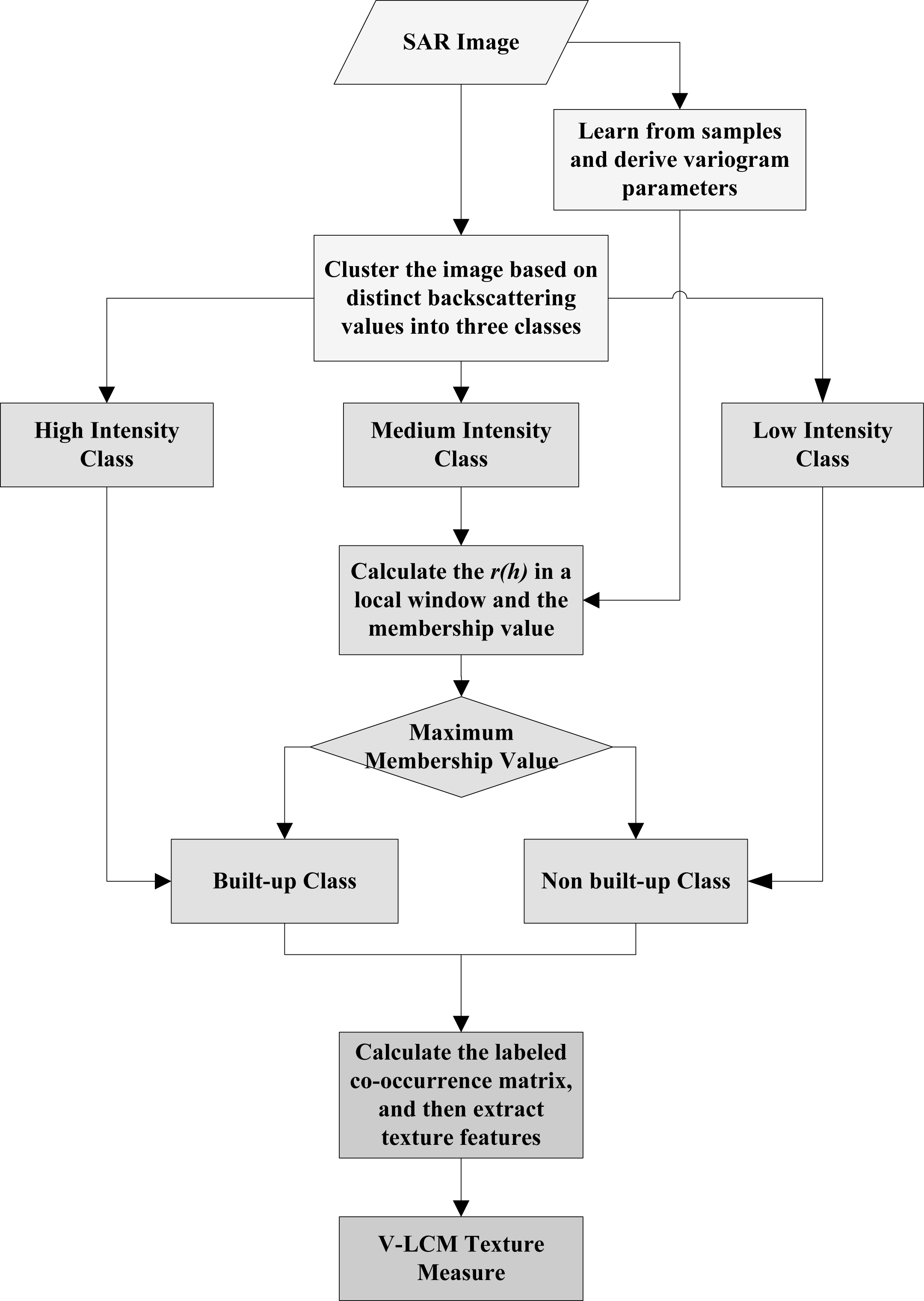
In [13], we propose a Labeled Co-occurrence Matrix (LCM) technique to detect and extract the built-up areas from HR SAR images. The LCM technique is inspired by the distinct backscattering behaviors associated with different LC classes. Roughly speaking, the urban scenes can be characterized by three main types of backscattering: (i) low intensity, which corresponds to shadows, roads, possible presence of water, etc.; (ii) medium intensity, which corresponds to possible presence of vegetation, grassland, etc.; (iii) high intensity, which is mainly due to roof, façade and corner reflectors associated with buildings or to human infrastructures. Therefore, the LCM technique is started with an unsupervised clustering procedure on the amplitude of the SAR image by using the spatial fuzzy c-means algorithm (SFCM) [29] technique, and three clusters are considered corresponding to the three main types of backscattering. The obtained classes are denoted as the high intensity class C₁ with the prototype v₁, the medium intensity class C₂ with the prototype v₂, and the low intensity class C₃ with the prototype v₃, where v₁, v₂, v₃ are obtained cluster centers, and v₁ > v₂ > v₃. According to the maximum membership value, each pixel is assigned to one of the three backscattering classes. However, there is a considerable proportion of pixels in the class C₂ charactering the built-up areas. In order to identify them, the following equation is used to re-calculate the membership degree for each pixel s ∈ C₂:

$${\mu }^r(s)={\left(\sum _{j=1,3}{\left(\frac{\Vert I(s)-v_r\Vert }{\Vert I(s)-v_j\Vert }\right)}^2\right)}^{-1},r=1,3$$

(1)

Equation (1) is based on the underlying assumption that the prototype v₁ of the class C₁ represents the built-up class S_B, while the prototype v₃ of the class C₃ represents the non built-up class S_N. According to the maximum membership value, the pixels of the class C₂ are assigned either to the built-up class S_B or the non built-up class S_N. Then each pixel in the amplitude of SAR image is attached with a label and a membership value associated with a particular class.

Similarly to p(I(s_i), I(s_j)|d, θ), the function e(l(s_i), l(s_j)|d, θ) can be defined as the joint label distribution for a pair of pixels in a given distance d and direction θ within a local region. Specifically, the function e(l(s_i), l(s_j)|d, θ) is calculated by connecting the membership values of the pixels that one has a label l(s_i) and the other has a label l(s_j), s_i, s_j ∈ S with a conjunctive operator ∧. The textural information is specified by the matrix e[(l(s_i), l(s_j)|d, θ)]_L×L, where L is the number of labels, with diverse orientations and lag distances being involved.

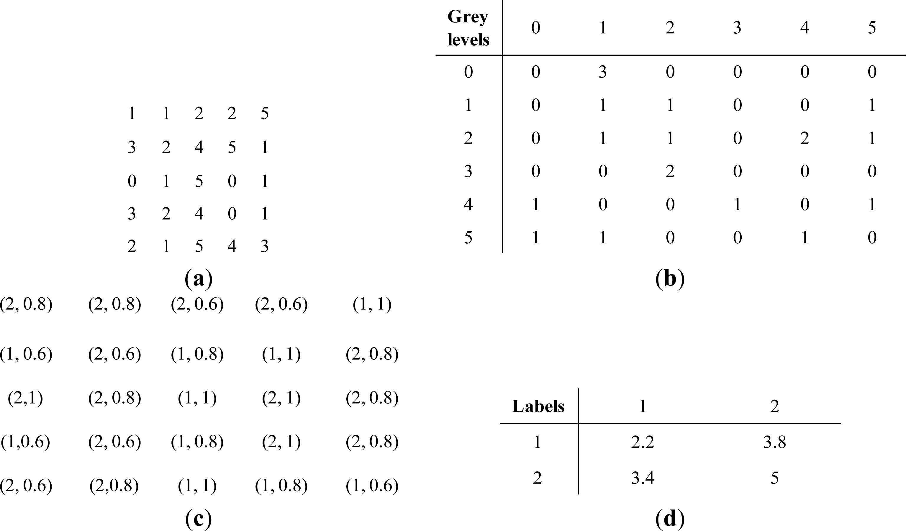
In order to illustrate the difference between the GLCM and LCM techniques, an example is shown in Figure 1. Figure 1a is a 5 × 5 digital image with grey levels: 0–5. The obtained grey level co-occurrence matrix [p_|d=1,θ=0°]_6×6 is given is Figure 1b, where the lag distance d = 1, and the orientation θ = 0°. Let us suppose that the 5 × 5 digital image can be transformed into the image shown in Figure 1c. Note that two classes are considered. The grey levels G = 3,4,5 are expected to belong to the first class, labeled by 1; whereas the grey levels G = 0,1,2 are expected to belong to the second class, labeled by 2. At this level, each pixel in Figure 1a is specified with a label and a membership value. The obtained labeled co-occurrence matrix [e_|d=1,θ=0°]_2×2 from Figure 1c with d = 1 and θ = 0° is shown in Figure 1d. The solutions for the computation of the matrix [e_|d=1,θ=0°]_2×2 are as follows:

$$\left[e_{|d=1,\theta =0°}(1,1)\right]=(0.8\wedge 1)+(0.8\wedge 1)+(0.8\wedge 0.6)=2.2$$

(2)

$$\left[e_{|d=1,\theta =0°}(1,2)\right]=(0.6\wedge 0.6)+(1\wedge 0.8)+(1\wedge 1)+(0.6\wedge 0.6)+(0.8\wedge 1)=3.8$$

(3)

$$\left[e_{|d=1,\theta =0°}(2,1)\right]=(0.6\wedge 1)+(0.6\wedge 0.8)+(0.8\wedge 1)+(0.6\wedge 0.8)+(0.8\wedge 1)=3.4$$

(4)

$$\begin{array}{l}\left[e_{|d=1,\theta =0°}(2,2)\right]=(0.8\wedge 0.8)+(0.8\wedge 0.6)+(0.6\wedge 0.6)+(1\wedge 0.8)+(1\wedge 0.8)+(1\wedge 0.8)\\ \hspace{0.17em}\hspace{0.17em}\hspace{0.17em}\hspace{0.17em}\hspace{0.17em}\hspace{0.17em}\hspace{0.17em}\hspace{0.17em}\hspace{0.17em}\hspace{0.17em}\hspace{0.17em}\hspace{0.17em}\hspace{0.17em}\hspace{0.17em}\hspace{0.17em}\hspace{0.17em}\hspace{0.17em}\hspace{0.17em}\hspace{0.17em}\hspace{0.17em}\hspace{0.17em}\hspace{0.17em}+(0.6\wedge 0.8)=5\end{array}$$

(5)

One can see from Figure 1 that the grey levels are replaced by the labels of the classes, and the joint grey-level distributions are replaced by the joint label distributions accordingly specified by the membership values. Note that the dimension of [p_|d=1,θ=0°]_6×6 is even larger than the size of the given digital image; whereas the dimension of [e_|d=1,θ=0°]_2×2 is reduced greatly and just chosen as the number of the considered classes.

The disadvantage of the LCM technique is that, since only grey level information is used, it cannot detect built-up areas with low intensities. To be specific, the pixel s ∈ C₂ is attached to the class that it is closer to in the grey space. When the pixel characterizing the built-up areas have considerable distances to the high-backscattering prototype and the low-backscattering prototype in the grey space, the fuzziness of its belongingness increases, resulting in poor detection accuracy eventually. As a result, an improved understanding between the built-up areas and other LC classes is required.

4. Proposed Method

4.1. Semivariogram (or Variogram)

Matheron introduced spatial statistics into the theory of regionalized variables [30]. The theory of the regionalized variable provides a concise and coherent methodology for describing and analyzing spatially distributed data [31]. The gray-level value of a pixel in remote sensing images can be considered as a regionalized variable, satisfying the following conditions:

$$E(I(s+\mathbf{h})-I(s))=0$$

(6)

$$\mathit{Var}(I(s+\mathbf{h})-I(s))=2\gamma (\mathbf{h})$$

(7)

where E(·) is the expectation function, Var(·) is the variance function, h is a vector including the lag h and the orientation θ, γ(h) is the semivariance at lag h. Equation (6) implies that the expectation of the regionalized variable does not vary spatially. In Equation (7), the variance of two regionalized variables, being independent of concrete spatial locations, only depends on the distance between them. The above two equations constitute the Matheron’s intrinsic hypothesis. Based on the intrinsic hypothesis, the semivariance for a given lag h is estimated by the following equation:

$$\gamma (\mathbf{h})=\frac{1}{2N(\mathbf{h})}\sum _{i=1}^{N(\mathbf{h})}{(I(s+\mathbf{h})-I(s))}^2$$

(8)

where N(h) is the number of the pairs of observations separated by the lag h. In fact, for a remote sensing image with a very large scene, the mean values of the variables usually vary from one part to another. In that case, the Matheron’s intrinsic hypothesis cannot be satisfied. Therefore, the variable is usually supposed to be locally stationary. At this level, the variable is assumed to satisfy the quasi-intrinsic hypothesis.

A further simplification of Equation (8) uses the absolute value [11], which may provide a good computational efficiency and robust performance, given by:

$$\gamma (\mathbf{h})=\frac{1}{2N(\mathbf{h})}\sum _{i=1}^{N(\mathbf{h})}\left|I(s+\mathbf{h})-I(s)\right|$$

(9)

The semivariance has distinct directivities. In this paper, the omni-directional semivariance γ^*(s; h) calculated in a local neighborhood is used, given by:

$${\gamma }^{*}(s;h)=\frac{1}{4}({\gamma }_{0°}(s;h)+{\gamma }_{45°}(s;h)+{\gamma }_{90°}(s;h)+{\gamma }_{135°}(s;h))$$

(10)

where γ_0°(s; h), γ_45°(s; h), γ_90°(s; h) and γ_135°(s; h) are the semivariace calculated in a particular direction by using Equation (9). Since γ^*(s; h) takes four directions into account, it may reduce the influence caused by the orientations.

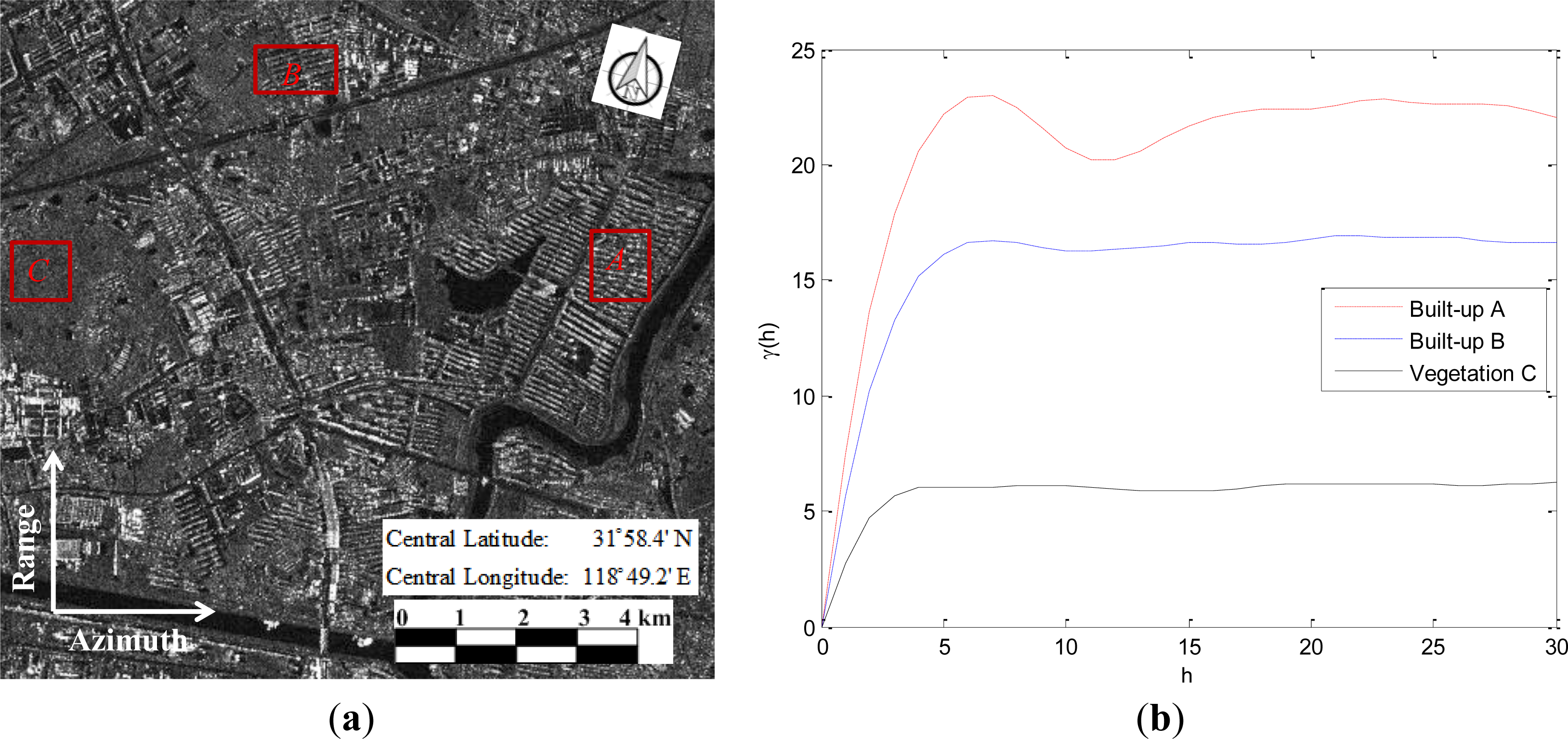
Semivariogram (or variogram) characterizes the distribution of the regionalized variable. It is obtained by connecting γ^*(h) with each discrete lag h, increasing from h = 0 to h_max (e.g., h_max = 30). In dealing with SAR images, a common way is to divide the data into a few groups that each one is associated with a particular physical surface (e.g., water, vegetation, built-up class). Then semi-variogram is constructed on each group, and the parameters are derived accordingly. Figure 2 presents an example on a SAR image of an urban scene, where dense buildings can be found. Two built-up regions in different backscattering values, marked by A and B, and a vegetation region marked by C are selected. The experimental variograms h − γ^*(h) on the three regions are plotted in the Figure 2b. There are two important parameters in the variogram: the range of influence a and the sill c. The range of influence stands for the lag at which the data samples become independent. The sill c represents the maximum of the non-similarity of the data. In order to derive the parameters automatically, Ramstein et al. [32] proposes a method to approximately compute the range and the sill:

$$a=-{\left(\text{log}(1-\gamma (1)/E\left(I{(s)}^2\right)\right))}^{-1}$$

(11)

$$c=\underset{h\to \infty }{\text{lim}}\gamma (h)=\underset{h\to \infty }{\text{lim}}\frac{1}{2}\left\{E\left\{{\left(I(s+h)-I(s)\right)}^2\right\}\right\}=E\left(I{(s)}^2\right)$$

(12)

Equations (11) and (12) actually are derived from an exponential variogram: γ(h) = c(1 − exp(−h/a)). The empirical models (e.g., spherical, exponential, and linear) can only describe simple and homogeneous scenes. It cannot characterize the regions featuring extreme heterogeneity. In remote sensing images, the man-modified surfaces (e.g., urban scenes) usually present repetitive or multi-frequency spatial patterns (e.g., the variogram for Region A in Figure 2b). With regard to the computation of the parameters â_b and ĉ_b on the built-up class, a simple procedure is proposed in [12]. The steps are as follows:

• Step 1: Take the Gauss filter to smooth the experimental h − γ^*(h) curve, and then compute the forward and backward difference of γ^*(h) by the following equation:

  $$\{\begin{array}{l}\Delta {\gamma }^{*}(h_i)={\gamma }^{*}(h_i)-{\gamma }^{*}(h_i-1)\\ \nabla {\gamma }^{*}(h_i)={\gamma }^{*}(h_i)-{\gamma }^{*}(h_i+1)\end{array}$$

  (13)
  where h_i = 2, ⋯, h_max − 1.

• Step 2: Find ĥ_i that satisfies the following conditions:

  $$\{\begin{array}{l}\Delta {\gamma }^{*}(h_i)>0\\ \nabla {\gamma }^{*}(h_i)<0\end{array}$$

  (14)
  Then, the range â_b and the sill ĉ_b are defined as:
  $${\widehat{a}}_b=\underset{i=1,2,\dots }{\text{min}}\left\{{\widehat{h}}_i\right\},\hspace{0.17em}\hspace{0.17em}{\widehat{c}}_b={\gamma }^{*}({\widehat{a}}_b)$$

  (15)

The variogram associated with the vegetation class can be taken as the spherical model (e.g., the variogram for Region C in Figure 2b) with the parameters â_v and ĉ_v. In the present work, â_v is not a mandatory parameter since â_v < â_b. The sill ĉ_v is given as the maximum of γ^*(h):

$${\widehat{c}}_v=\underset{h_i}{\text{max}}({\gamma }^{*}(h))$$

(16)

4.2. Variogram Integrated Labeled Co-Occurrence Matrix Texture Features

Figure 2 illustrates that each LC type is associated with a specific spatial variability structure. Particularly, Region B and Region C present similar backscattering values; however their spatial variability structures are distinct. Therefore, we will take the variogram into account to improve the LCM technique presented in the previous section. For discrimination, the enhanced version proposed in this paper is called V-LCM.

In the initial step, the amplitude of a SAR image is clustered into three classes: the high intensity class C₁, the medium intensity class C₂, and the low intensity class C₃, by using the spatial FCM technique.

The built-up class S_B and the non built-up class S_N satisfy S_B ∪ S_N = S and S_B ∩ S_N = ø. Assume that the pixel s ∈ C₁ belongs to the built-up class S_B, and the pixel s ∈ C₃ belongs to the non built-up class S_N, having C₁ ⊂ S_B and C₃ ⊂ S_N. The key of the approach is to assign the pixel s ∈ C₂ to the classes S_B or S_N.

Different distribution patterns and backscattering coefficients of built-up regions in SAR images are usually associated with variograms of distinct shapes and parameters. Therefore, in a given SAR image, we empirically select two typical built-up regions R_B1 and R_B2, and a vegetation region R_v. R_B1 should be in strong backscattering values and of great spatial variation (e.g., Region A in Figure 1a), while R_B2 should be in low backscattering values and of weak spatial variation (e.g., Region B in Figure 1a). It is expected that the parameters derived from the two training samples R_B1 and R_B2 are the lower bounds of the ones derived from the regions with the similar characteristics respectively. Let us denote ${\widehat{c}}_b^h$ be the sill for the region R_B1, â_b and ${\widehat{c}}_b^l$ be the range and the sill for the region R_B2, and ĉ_v be the sill for the region R_v. These parameters can be estimated by using the procedures introduced in Section 4.1, respectively.

Let us suppose that the class S_B is characterized by the membership function μ_SB: S_B → [0,1], while S_N is characterized by the membership function μ_SN: S_N → [0,1]. The term γ(s; â_b), s ∈ C₂ is the semivariance computed in a local window by using Equation (10), where the pairs of pixels are separated by the distance â_b. The size of the local window is supposed to be three to five times longer than the range â_b [10]. Thus, w_v = 4â_b is used.

The membership function characterizing the class S_B is given by:

$${\mu }_{S_B}=\{\begin{array}{ll}1,\hfill & \mathit{if}\hspace{0.17em}\hspace{0.17em}s\in C_1,\hspace{0.17em}\hspace{0.17em}\hspace{0.17em}\hspace{0.17em}\hspace{0.17em}\hspace{0.17em}\hspace{0.17em}\text{or}\hspace{0.17em}\hspace{0.17em}\hspace{0.17em}\hspace{0.17em}\hspace{0.17em}\hspace{0.17em}s\in C_2,\hspace{0.17em}\hspace{0.17em}\gamma (s;{\widehat{a}}_b)\ge {\widehat{c}}_b^h\hfill \\ {\left(1+{\left(\frac{\left|\gamma (s;{\widehat{a}}_b)-{\widehat{c}}_b^l\right|}{\gamma (s;{\widehat{a}}_b)-{\widehat{c}}_v}\right)}^2\right)}^{-1},\hfill & \mathit{if}\hspace{0.17em}\hspace{0.17em}s\in C_2,\hspace{0.17em}\hspace{0.17em}\gamma (s;{\widehat{a}}_b)<{\widehat{c}}_b^h?\hfill \end{array}$$

(17)

The membership function characterizing the class S_N is given by:

$${\mu }_{S_N}=\{\begin{array}{ll}1,\hfill & \mathit{if}\hspace{0.17em}\hspace{0.17em}s\in C_3,\hspace{0.17em}\hspace{0.17em}\hspace{0.17em}\hspace{0.17em}\hspace{0.17em}\hspace{0.17em}\hspace{0.17em}\text{or}\hspace{0.17em}\hspace{0.17em}\hspace{0.17em}\hspace{0.17em}\hspace{0.17em}\hspace{0.17em}s\in C_2,\hspace{0.17em}\hspace{0.17em}\gamma (s;{\widehat{a}}_b)\ge {\widehat{c}}_v\hfill \\ {\left(1+{\left(\frac{\left|\gamma (s;{\widehat{a}}_b)-{\widehat{c}}_v\right|}{|\gamma (s;{\widehat{a}}_b)-{\widehat{c}}_b^l|}\right)}^2\right)}^{-1},\hfill & \mathit{if}\hspace{0.17em}\hspace{0.17em}s\in C_2,\hspace{0.17em}\hspace{0.17em}\gamma (s;{\widehat{a}}_b)<{\widehat{c}}_v?\hfill \end{array}$$

(18)

According to the maximum membership value, each pixel s ∈ S, is assigned either to the class S_B with the memberships values μ_SB or to the class S_N with the memberships values μ_SN. At this level, the amplitude of the SAR image is transformed into a label—fuzzy image I_FL:

$$I_{FL}=\left\{\left(l(s),{\mu }_{S_m}(s)\right);s\in S,l(s)\in \{1,2\},{\mu }_{S_m}(s)\in [0,1],m\in \{B,N\}\right\}$$

(19)

where the pixel belonging to the class S_B is labeled with l(s) = 1, and l(s) = 2 for the class S_N.

The values in the matrix [e(l(s_i), l(s_j)|d, θ)]_L×L are obtained by combining the membership values in a conjunctive way. In the fuzzy set theory, the fuzzy operator t-norm T has a conjunctive behavior, which is a mapping T: [0,1]×[0,1]→[0,1]. The frequently used T operators are [33]:

(1)

T(t₁, t₂) = min(t₁, t₂)

(2)

T(t₁, t₂) = t₁ ·t₂

(3)

T(t₁, t₂) = 1 − min{1,((1 − t₁)ⁿ + (1 − t₂)ⁿ)^1/n}, n ≥ 1

where t₁ and t₂ are variables in the interval [0,1]. In fact, the operator provides the largest values among T operators. The matrix [e(l(s_i), l(s_j)|d, θ)]_L×L can be computed by using these T operators.

From the resulting matrix, the autocorrelation feature is extracted, and given as follows:

$$\mathit{auto}=\sum _{l(s_i)}\sum _{l(s_j)}l(s_i)\cdot l(s_j)\cdot e(l(s_i),l(s_j))$$

(20)

Figure 3 displays a block scheme of the procedure for computing the proposed V-LCM texture measure. Since the spatial statistics of the land-covers is considered, the robustness and effectiveness of the proposed V-LCM technique will be greatly improved compared with the original LCM technique.

4.3. Built-up Area Extraction

Based on the V-LCM texture measure, the procedure for the detection and extraction of the built-up areas in a SAR image is given as follows:

(1)

Pre-processing: Speckle noise significantly hinders the interpretation of a SAR image. Hence, the noise should be filtered. Various filtering techniques have been developed to enhance the image quality. In terms of the analysis of the urban landscapes in a SAR data, structure-preserving speckle suppression techniques are required. The Enhanced Frost filter [34], being able to preserve the structures and texture information both in homogeneous and heterogeneous areas, is used in the proposed method.

(2)

Texture modeling and extraction: The spatial FCM technique is applied to cluster the amplitude of the SAR image, and a 5 × 5 window is incorporated into local membership function for the removal of noisy regions or spurious blobs. Two typical built-up samples and a vegetation sample are manually selected. The size of the samples should be large enough to achieve reliable statistics. Following the procedure shown in Figure 3, the texture feature can be extracted. However, before that, several parameters need to be estimated in the implementation of the V-LCM technique. First, an appropriate local window w_f should be considered, and w_f = 15 × 15 may be appropriate for an image having a resolution of about 3 m. Moreover, in a large scene of SAR image, the patterns of the built-up regions are usually diverse and arranged irregularly. Single orientation inadequately represents the texture pattern. Therefore, we take the four directions θ = {0°, 45°, 90°, 135°} into account, and the texture measure is taken as the average of the four components. In terms of the distance d, d = 4 was found to better represent the texture information in experiments.

(3)

Classification and Post-processing: The autocorrelation feature computed from the V-LCM technique is sufficient enough to highlight the presence of the built-up areas in a SAR image. The classification is implemented by using a simple Otsu thresholding method on the texture measure. Finally, morphological operations are used on the obtained classification result to remove sparse and spurious pixels.

5. Experimental Results and Discussions

In order to demonstrate the effectiveness of the proposed method, we use subsets of a COSMO-SkyMed (CSK) image referring to Hangzhou, China, and of two TerraSAR-X (TSX) images referring to Nanjing, China, and Barcelona, Spain, acquired in Stripmap mode. Some basic properties about the images are listed in

Table 1. Properties of the synthetic aperture radar (SAR) images used in this paper.

Test site	Sensors	Resolution	Acquisition Date	Polarization
Nanjing, China	TerraSAR-X	2.75 m	4 March 2008	VV
Barcelona, Spain	TerraSAR-X	3 m	15 May 2011	HH
Hangzhou, China	COSMO-SkyMed	3 m	8 January 2008	HH

. Quantitative results are computed by the comparisons with manual ground reference data. The reference samples used in the experiments have been taken manually from both the original SAR images and the corresponding high resolution optical images. The numerical values of the ground truths are listed in

Table 2. Ground truth data used in accuracy assessment.

Image Data	Nanjing, China	Barcelona, Spain	Hangzhou, China
No. of Built-up pixels	4,123,264	3,794,725	1,880,875

.

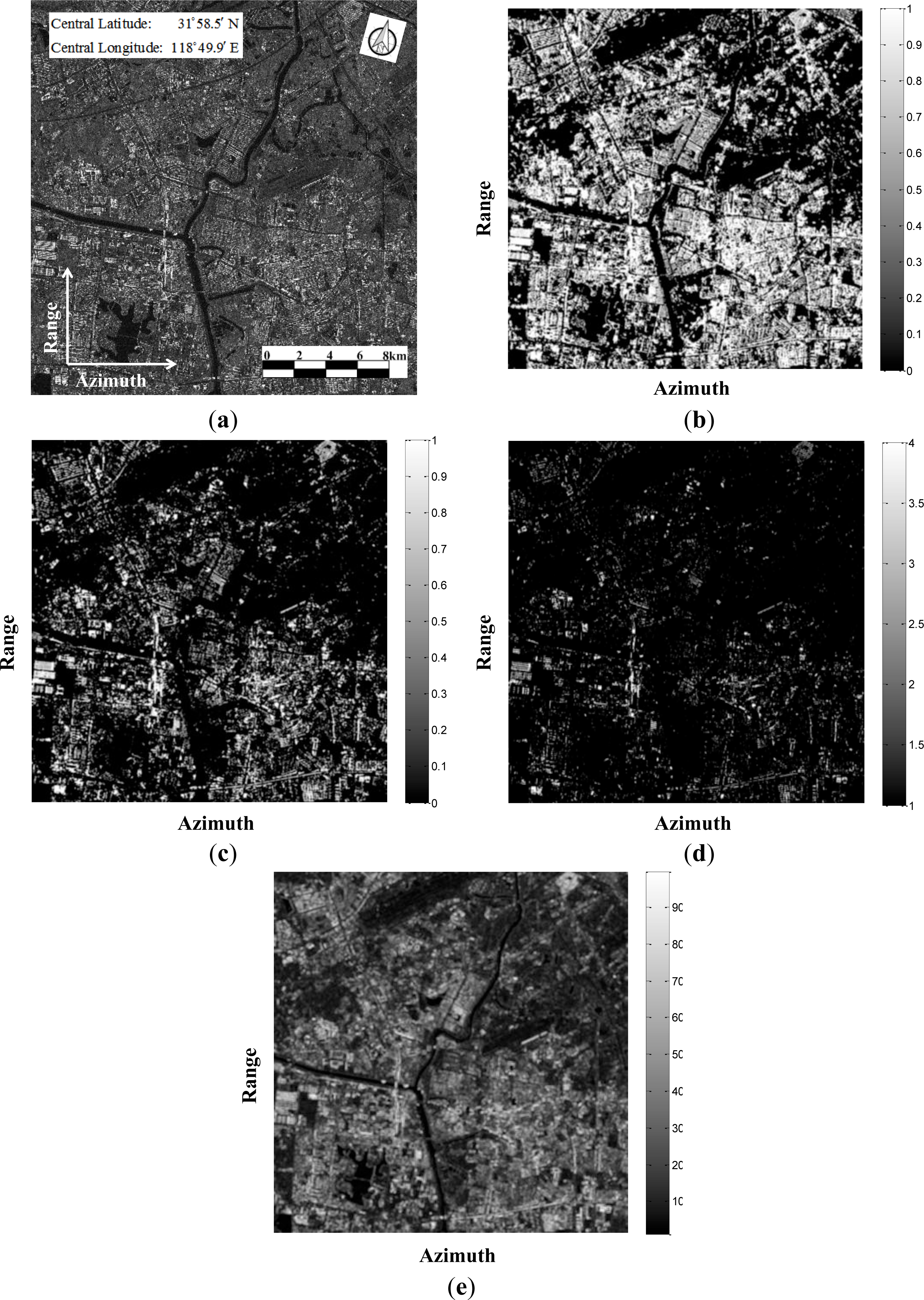
The first experiment is to compare the performance of different texture measures. The SAR image shown in Figure 4a is a portion of the city of Nanjing, China. It is a sub-scene from a product in spatially enhanced (SE) single polarizations, and enhanced ellipsoid corrected projection (EEC). The number of looks for this data is four. The size of the subset is 2883×2949. The scene mainly includes water (lake and river), vegetation, buildings, and a portion of an airport. The city of Nanjing has a high population density, which can be confirmed by the dense built-up areas. The patterns of the clusters of buildings are quite complicated. For instance, there are well-planned high-rise buildings, dense or scattered bungalows, plant buildings, etc. Figure 4b–e presents the autocorrelation features extracted by using the proposed V-LCM technique, the LCM technique and the traditional GLCM technique, and a semivariance feature image. The parameters used in computing these features are: the window size w_v = 25 × 25, the window size w_f = 17 × 17, the range â_b = 6, and the quantized grey levels G = 2. One can see that V-LCM technique (see Figure 4b) achieves the most visually appealing results compared with other features, since almost all the built-up areas found in the scene have been highlighted. The LCM technique (see Figure 4c) and the variogram descriptor (see Figure 4e) have similar textural representation abilities; while the traditional GLCM technique (see Figure 4d) behaves worst in characterizing the built-up areas. The classification results based on the obtained features are shown in Figure 5.

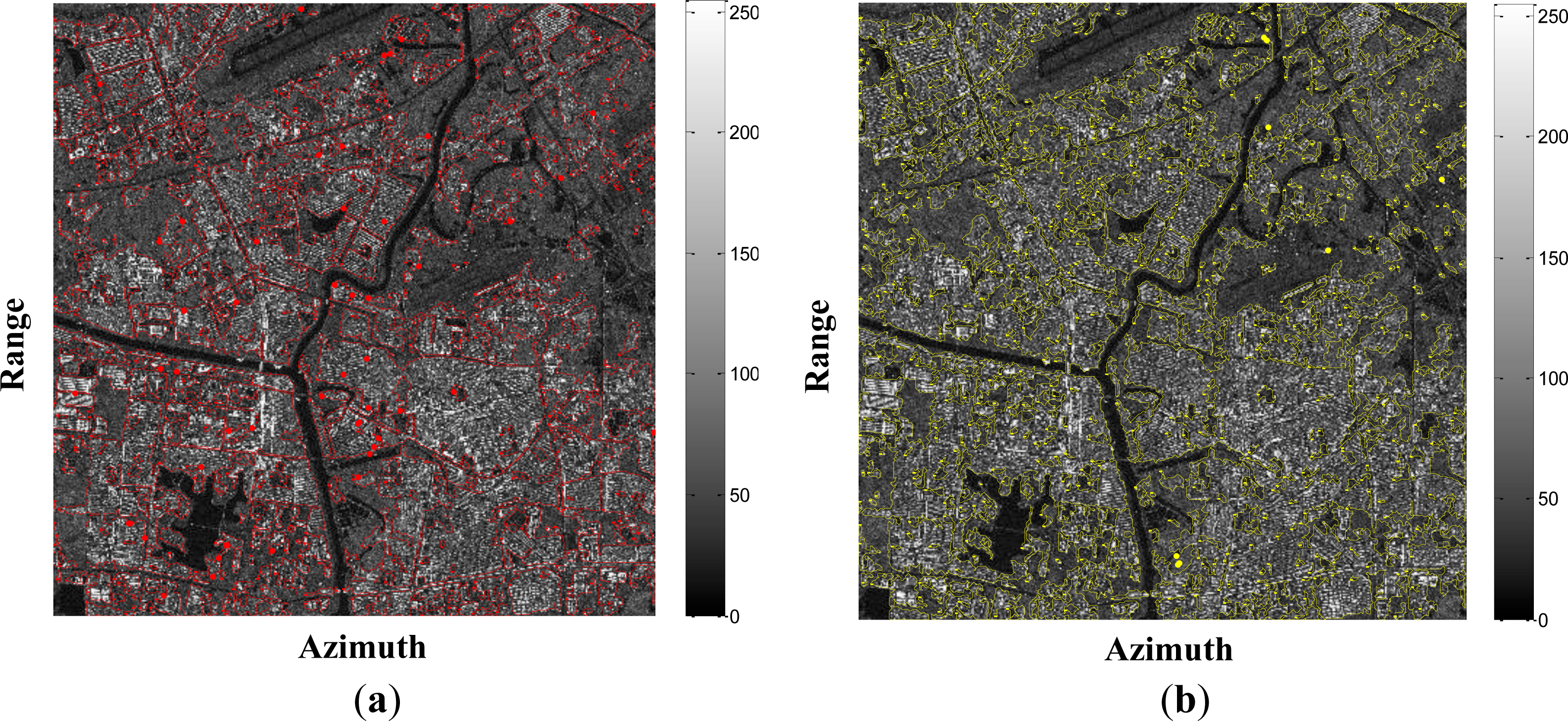
Referring to [35], the manually extracted reference map is shown in Figure 5a. The extraction result obtained by using the proposed V-LCM technique is shown in Figure 5b. Compared with the ground reference, almost all the built-up areas have been effectively extracted. The overall detected pixels are 4,656,346 pixels (4,019,358 correctly detected pixels and 636,988 false detected pixels). A quantitative comparison of the accuracies by using different texture measures are listed in

Table 3. Comparisons of classification accuracies by using different texture measures. (a) Classification accuracies on the TSX image of Nanjing (China); (b) classification accuracies on the TSX image of Barcelona (Spain); (c) classification accuracies on the CSK image of Hangzhou (China).

Methods	Detection Accuracy (%)	False Alarm (%)	Overall Accuracy (%)
Proposed V-LCM	97.48	13.68	91.29
LCM	71.56	8.04	83.17
GLCM	39.80	7.39	69.26
Variogram	61.89	10.51	77.99
(a)
Methods	Detection Accuracy (%)	False Alarm (%)	Overall Accuracy (%)
Proposed V-LCM	97.24	16.01	91.15
LCM	85.15	9.78	89.89
GLCM	80.35	11.68	87.42
Variogram	87.19	12.27	89.61
(b)
Methods	Detection Accuracy (%)	False Alarm (%)	Overall Accuracy (%)
Proposed V-LCM	94.12	28.30	91.63
LCM	74.62	23.77	90.54
GLCM	53.48	13.65	89.31
Variogram	78.36	20.16	92.72
(c)

. The detection accuracy by using the proposed V-LCM technique is 97.48%, where 4,019,358 correctly detected pixels were out of 4,123,264 pixels. The false alarm rate is 13.68%, where 636,988 false detected pixels were out of 4,656,346 overall detected pixels. The overall errors are 740,894 pixels which are 636,988 false detected pixels plus 103,906 missed pixels, resulting in 8.71% error rate (740,894 errors out of the overall 8,501,967 pixels of the image). The overall accuracy can be obtained accordingly, and is 91.29%. Note that the classifications on Figure 4c,d were using the procedure introduced in [13]. In terms of the semivariance image in Figure 4e, the FCM technique was applied to the cluster feature image with two clusters involved [12]. By comparison, the detection accuracies obtained from the LCM technique and the variogram technique are 71.56% and 61.89%, respectively. However, it is merely 39.80% for the GLCM technique. Hence, the proposed V-LCM technique achieved the best performance. The processing times for this data by using different techniques are listed in

Table 4. Comparisons of processing times on each data by using different techniques and the hardware conditions. (a) Processing times by using different techniques on each data; (b) software platform and hardware conditions.

Methods	Nanjing, China (min)	Barcelona, Spain (min)	Hangzhou, China (min)
Proposed V-LCM	22.8	25.5	24.3
LCM	16.1	16	16.7
GLCM	11.7	11.5	12.2
Variogram	9.4	12.7	10.7
(a)

Software	Operation Systems	CPU	RAM
Matlab 7.11.0.584	Windows 8 × 64 bit	Intel i5-3350p 3.10 GHz	4 GB
(b)

. The hardware platform used is shown in Table 4b. Though the time consuming for the proposed V-LCM technique is not satisfactory compared other methods, it can be tolerate.

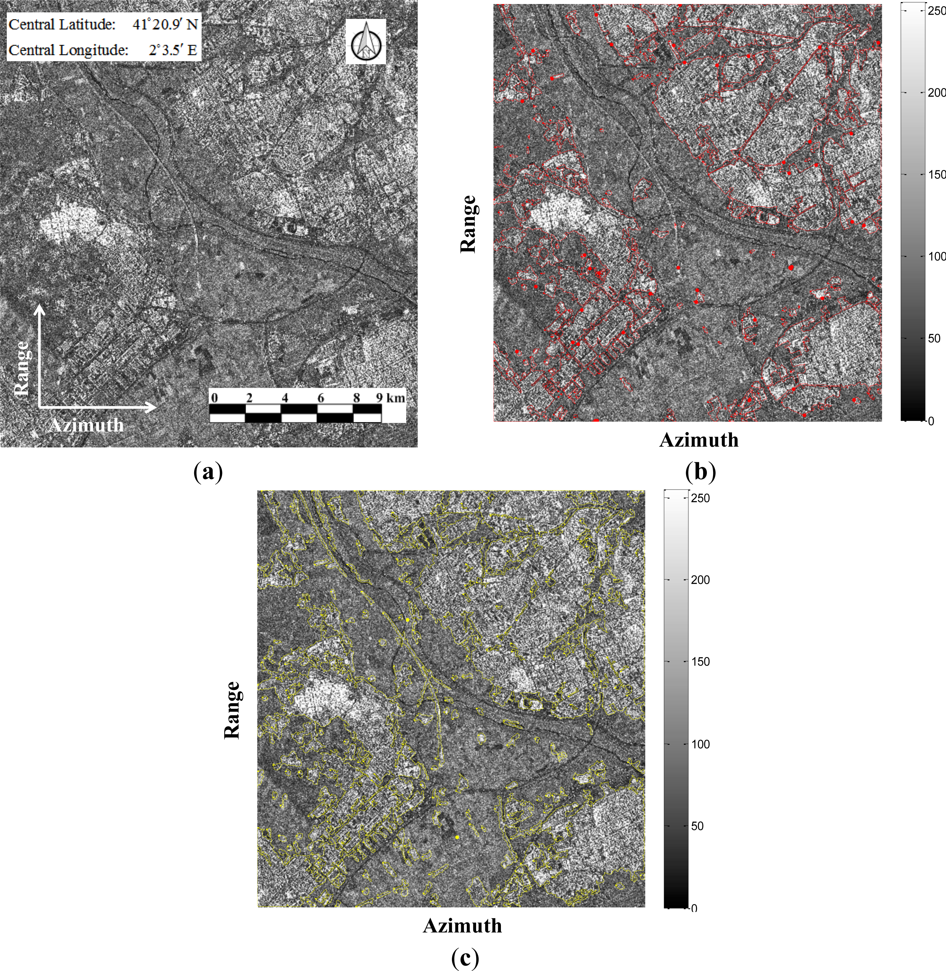
The second scene is a portion of the city of Barcelona, which is available in [36]. It is acquired in ascending orbit with the incidence angle 35.2°, and on 15 May 2011. It is in single polarizations, and UTM, WGS 84 projection. The depicted scene is the urban and suburban area around the airport of Barcelona, Spain. One can see from Figure 6a that there are three densely populated areas, and a large area with crop fields among them. The test image is of size 2912×3135. The parameters used are: the range â_b = 7, window size w_v = 29 × 29, window size w_f = 15 × 15, and quantized grey levels G = 2. The processing times for this data by using different techniques can refer to Table 4a. Figure 6b is the reference map. The extracted built-up areas by using the proposed technique are shown in Figure 6c. One can see that some false areas are detected. They are mainly caused by the high-speed roads, crop fields and vegetation, which present radar signatures similar to those of buildings. The qualitative comparisons of the results obtained from different techniques are shown in Table 3b. The proposed V-LCM technique achieves 97.24% detection accuracy, which is compared with 87.19% for the variogram technique and 85.15% for the LCM technique. The detection accuracy for the GLCM technique is only 80.35%. The omission errors are mainly due to the large factory buildings featuring flat roofs, where the radar signals are scattered away from the sensor. Thus, no energy is contributing to these areas resulting in low backscattering coefficients.

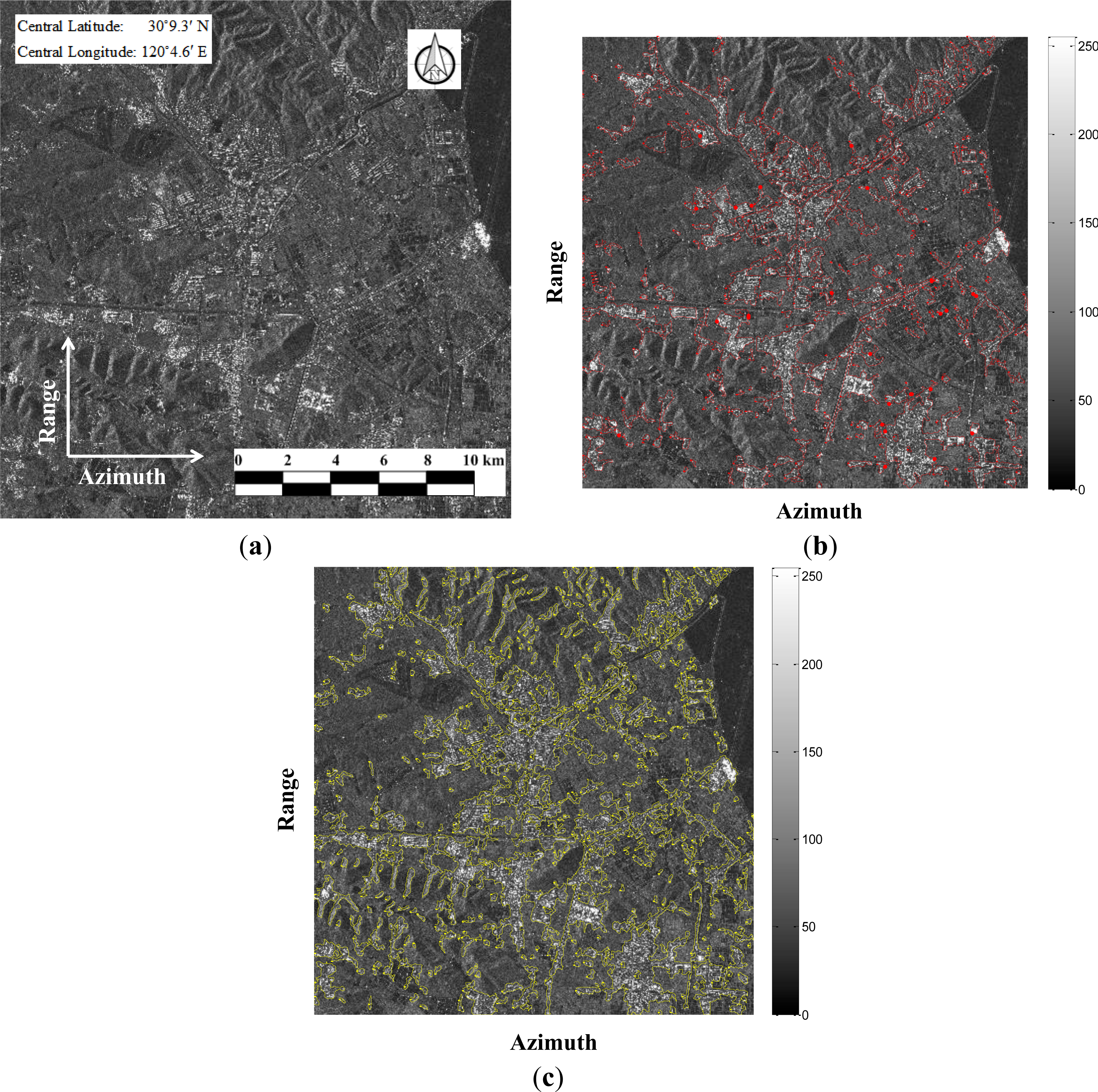
The third scene is a portion of the city of Hangzhou, China. It is a single polarization, and geocoded ellipsoid corrected (GEC) product. The number of looks for this data is three. The size of the image is 3078 × 3141. The landscape covers the river, crop fields, mountains, vegetation, and scattered small or large concentrated built-up areas. The parameters used in this example are: range â_b = 7, window size w_v = 25 × 25, window size w_f = 15 × 15, and quantized grey levels G =2. The processing times for this scene by using different techniques can refer to Table 4a. The reference map is shown in Figure 7b. The classification result by using the proposed V-LCM technique is shown in Figure 7c. By comparison of Figure 7b,c, a portion of false areas associated with mountain regions are detected due to the similar backscattering coefficients. Table 3c provides the quantitative results by using different techniques. It can be learned that the proposed V-LCM technique achieves the best performance (94.12% detection accuracy), and the GLCM technique remains the worst (53.34% detection accuracy). The LCM and the variogram techniques achieve similar detection results with detection accuracies 74.62% and 78.36%, respectively.

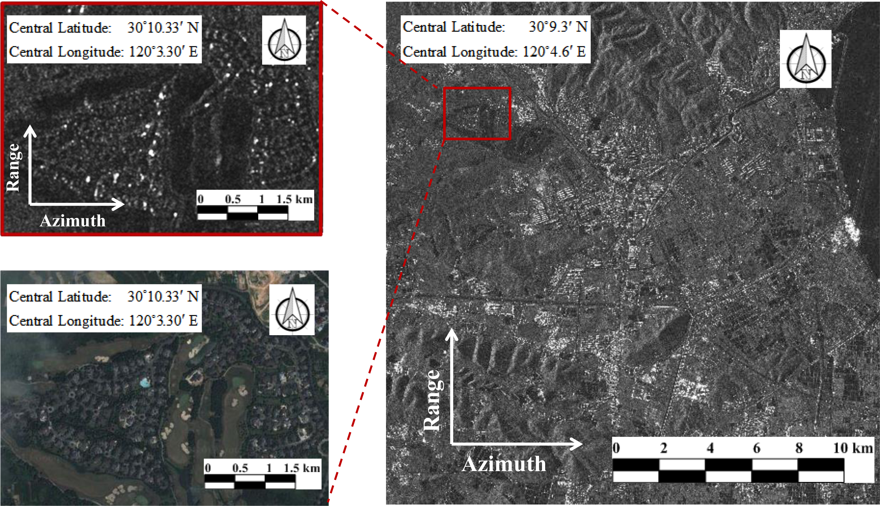
Since the spatial variety structures of the LC classes are considered, the proposed V-LCM technique shows very high detection rates in all cases. It is robust regardless of the backscattering variation, and can effectively indentify dense or scattered settlements with different characteristics. A limitation of the proposed method is related to the detection of the low-intensity built-up areas. In this case, the tuning of parameters may result in the false detection of mountains or other LC classes. Another critical situation is for built-up areas, featuring very low intensity and weak non-similarity. Figure 8 shows an example found in the Hangzhou scene, where the built-up areas were not detected by all methods. The omitted area is zoomed-in and displayed together with the optical image from the Google Earth. One can see that trees are interspersed within the villas. When the radar system illuminates these regions, most of the signal is reflected by the plants and only few contributions are scattered by the buildings. Thus, these regions present a low intensity and very similar spatial variety structures to the vegetation. By comparison, the LCM technique can work well on built-up regions appearing bright. Since only grey information is used, it may be susceptible to the backscattering variation.

The detection accuracies, false alarms and overall accuracies obtained by using considered techniques on the three test images are shown in Table 3. One can see that as expected the proposed technique achieved higher detection accuracies and overall accuracies; however, false alarms were produced. Several issues are associated with the problem. Firstly, some vegetations present high intensity values (e.g., woods), resulting in the difficulties in discrimination. Secondly, some man-made structures such as roads, bridges, cars, found in the scene may cause strong backscattering because of the double bounce effects. Thirdly, the foreshortening and layover effects occurred in the mountains areas usually cause very strong backscattering. However, the errors caused by the mountainous can be eliminated by the use of auxiliary information (e.g., the geocoded incidence angle map (GIM)) [24].

6. Conclusions

In this paper, a novel texture measure for detecting the built-up areas in high resolution (HR) synthetic aperture radar (SAR) images is proposed. The variogram integrated labeled co-occurrence matrix (V-LCM) texture measure is obtained by combining the labeled co-occurrence matrix (LCM) method with the analysis of the spatial variability structure associated with each land-cover (LC) type in SAR images. Based on the observations of backscattering behaviors of different land-cover classes, only the built-up regions appearing bright can be identified by using the LCM technique. In SAR images, some built-up areas in medium and relatively low intensity may have similar backscattering coefficients with vegetations, resulting in confusions. An improved understanding between the built-up areas and other land-cover classes is required. The variogram provides a way to analyze the spatial variability of the surface, which actually reflects the spatial correlation. An example shown in paper illustrates that the vegetation and built-up areas, though they present similar grey values, have distinct spatial structures based on the variogram analysis. Therefore, in a given SAR image, we manually select three typical LC samples and train them to obtain the required parameters. Fuzzy membership functions can be established based on the acquired parameters, which are used to describe the built-up class and non built-up class separately. The co-occurrence matrix is defined in a conjunctive way by using the membership values. Finally, the classification procedure is performed on the autocorrelation feature image by using simple Otsu thresholding technique. The proposed V-LCM technique has been tested on two TerraSAR-X images and a COSMO-SkyMed image, and compared with other texture measures. The V-LCM technique achieved the best performance in all cases. The effectiveness and robustness has been confirmed.

There are some issues associated with the V-LCM technique in comparison with other considered texture measures. First, by comparison with the LCM technique, the V-LCM technique is improved greatly in characterizing the built-up areas in a SAR image regardless of the backscattering variation. The built-up areas in medium and relatively low intensity can be appropriately identified. Second, the labeled co-occurrence matrix is just chosen as the number of the considered classes. In this paper, two classes are used, specified by the built-up class and the non built-up class. In terms of the GLCM technique with grey values being quantized into 2-levels, poor classification accuracies were obtained in all cases because of the considerably lost image information. Finally, the variogram technique achieves similar detection and overall accuracy with the LCM technique. However, since only the spatial structure information of the surface is used, the variogram technique is not robust and effective as the proposed V-LCM technique.

The test images contain complex landscapes which provide a challenging benchmark for the proposed method. Note that even if it can effectively indentify the built-up areas with the highest detection and overall accuracies, false alarms are present in the final map. The false alarms are mainly due to mountains, roads, and the vegetation found in the scenes, which can appear bright and with textures being similar to built-up areas in some specific cases. Therefore, the future work should focus on better eliminating the false alarms, although proper post-processing techniques can be considered or the auxiliary information (e.g., the geocoded incidence angle map (GIM) for elimination of mountain regions) can be used.

References

- Lu, D.; Tian, H.; Zhou, G.; Ge, H. Regional mapping of human settlements in southeastern China with multisensor remotely sensed data. Remote Sens. Environ 2008, 112, 3668–3679. [Google Scholar]
- Roth, A.; Hoffmann, J.; Esch, T. TerraSAR-X: How can High Resolution SAR Data Support the Observation of Urban Areas. Proceedings of the ISPRS WG VII/1 “Human Settlements and Impact Analysis”,” 3rd International Symposium Remote Sensing and Data Fusion Over Urban Areas (URBAN 2005) and 5th International Symposium Remote Sensing of Urban Areas (URS 2005), Tempe, AZ, USA, 14–16 March 2005.
- Impagnatiello, F.; Bertoni, R.; Caltagirone, F. The SkyMed/COSMO System: SAR Payload Characteristics. Proceedings of 1998 IEEE International Geoscience and Remote Sensing Symposium, Seattle, WA, USA, 6–10 July 1998; pp. 689–691.
- Roth, A. TerraSAR-X: A New Perspective for Scientific Use of High Resolution Spaceborne SAR Data. Proceedings of the 2nd GRSS/ISPRS Joint Workshop on Remote Sensing and Data Fusion over Urban Areas, Berlin, Germany, 22–23 May 2003; pp. 4–7.
- Ferro, A.; Brunner, D.; Bruzzone, L. Building Detection and Radar Footprint Reconstruction from Single VHR SAR Images. Proceedings of the 2010 IEEE International Geoscience and Remote Sensing Symposium, Honolulu, HI, USA, 25–30 July 2010; pp. 292–295.
- Ferro, A.; Brunner, D.; Bruzzone, L. Automatic detection and reconstruction of building radar footprints from single VHR SAR images. IEEE Trans. Geosci. Remote Sens 2013, 51, 935–952. [Google Scholar]
- Ferro, A.; Brunner, D.; Bruzzone, L.; Lemoine, G. On the relationship between double bounce and the orientation of buildings in VHR SAR images. IEEE Trans. Geosci. Remote Sens. Lett 2011, 8, 612–616. [Google Scholar]
- Brunner, D.; Lemoine, G.; Bruzzone, L. Earthquake damage assessment of buildings using VHR optical and SAR imagery. IEEE Trans. Geosci. Remote Sens 2010, 48, 2403–2420. [Google Scholar]
- Henderson, F.; Xia, Z. SAR applications in human settlement detection, population estimation and urban land use pattern analysis: A status report. IEEE Trans. Geosci. Remote Sens 1997, 35, 79–85. [Google Scholar]
- Woodcock, C.E.; Strahler, A.H.; Jupp, D.L.B. The use of variograms in remote sensing I: Scene models and simulated images. Remote Sens. Environ 1988, 25, 323–348. [Google Scholar]
- Carr, J.R.; de Miranda, F.P. The semivariogram in comparison to the co-occurrence matrix for classification of image texture. IEEE Trans. Geosci. Remote Sens 1998, 36, 1945–1952. [Google Scholar]
- Zhao, L.J. The Study of Buildings Extraction in High Resolution SAR Images. Ph.D. Thesis, National University of Defense Technology, Changsha, China,. 2009. (In Chinese).. [Google Scholar]
- Li, N.; Bruzzone, L.; Chen, Z.P.; Liu, F. Labeled co-occurrence matrix for the detection of built-up areas in high-resolution SAR images. Proc. SPIE 2013. [Google Scholar] [CrossRef]
- Gouinaud, C.; Tupin, F. Potential and Use of Radar Images for Characterization and Detection of Urban Areas. Proceedings of the IEEE International Geoscience and Remote Sensing Symposium, Lincoln, NE, USA, 27–31 May 1996; pp. 474–476.
- He, C.; Xia, G.; Sun, H. An adaptive and iterative method of urban area extraction from SAR images. IEEE Trans. Geosci. Remote Sens. Lett 2006, 3, 504–507. [Google Scholar]
- Borghys, D.; Perneel, C.; Acheroy, M. Automatic detection of built-up areas in high-resolution polarimetric SAR images. Pattern Recognit. Lett 2002, 23, 1085–1093. [Google Scholar]
- Tison, C.; Nicolas, J.; Tupin, F. A new statistical model for Markovian classification of urban areas in high-resolution SAR images. IEEE Trans. Geosci. Remote Sens 2004, 42, 2046–2057. [Google Scholar]
- Dekker, R.J. Texture analysis and classification of ERS SAR images for map updating of urban areas in the Netherlands. IEEE Trans. Geosci. Remote Sens 2003, 41, 1950–1958. [Google Scholar]
- Gamba, P.; Massimilano, A.; Mattia, S. Robust extraction of urban area extents in HR and VHR SAR Images. IEEE J.-STARS 2011, 4, 27–34. [Google Scholar]
- Stasolla, M.; Gamba, P. Spatial indexes for the extraction of formal and informal human settlements from high-resolution SAR images. IEEE J.-STARS 2008, 1, 98–106. [Google Scholar]
- Haralick, R.M.; Shanmugam, K.; Dinstein, I.H. Textural features for image classification. IEEE Trans. Syst. Man Cybern 1973, 1, 610–621. [Google Scholar]
- Aiazzi, B.; Alparone, L.; Baronti, S. Measurement for SAR imagery. IEEE Trans. Geosci. Remote Sens 2004, 43, 619–624. [Google Scholar]
- Esch, T.; Thiel, M.; Schenk, A.; Roth, A.; Müller, A.; Dech, S. Delineation of urban footprints from TerraSAR-X data by analyzing speckle characteristics and intensity information. IEEE Trans. Geosci. Remote Sens 2010, 48, 905–916. [Google Scholar]
- Esch, T.; Heldens, W. Description of Settlement Patterns Using VHR SAR Data of the German TanDEM-X Mission. Proceedings of the 2012 IEEE International Geoscience and Remote Sensing Symposium, Munich,Germany, 22–27 July 2012; pp. 5737–5740.
- Shanmugan, K.S.; Narayanan, V.; Frost, V.S.; Stiles, J.A.; Holtzman, J. Textural features for radar image analysis. IEEE Trans. Geosci. Remote Sens 1981. [Google Scholar] [CrossRef]
- Dell’Acqua, F.; Gamba, P. Texture-based characterization of urban environments on satellite SAR images. IEEE Trans. Geosci. Remote Sens 2003, 41, 153–159. [Google Scholar]
- Dell’Acqua, F.; Gamba, P.; Trianni, G. Semi-automatic choice of scale-dependent features for satellite SAR image classification. Pattern Recognit. Lett 2006, 27, 244–251. [Google Scholar]
- Clausi, D. An analysis of co-occurrence texture statistics as a function of grey level quantization. Can. J. Remote Sens 2002, 28, 45–62. [Google Scholar]
- Chuang, K.S.; Tzeng, H.L.; Chen, S.; Wu, J.; Chen, T.J. Fuzzy c-means clustering with spatial information for image segmentation. Comput. Med. Imaging Graph 2006, 30, 9–15. [Google Scholar]
- Matheron, G. The Theory of Regionalized Variables and Its Applications; École Nationale Supérieure Des Mines de Paris: Paris, France, 1971. [Google Scholar]
- Oliver, M.; Webster, R.; Gerrard, J. Geostatistics in physical geography. Part I: Theory. Trans. Inst. Br. Geogr 1989, 14, 259–269. [Google Scholar]
- Ramstein, G.; Raffy, M. Analysis of the structure of radiometric remotely-sensed images. Int. J. Remote Sens 1989, 10, 1049–1073. [Google Scholar]
- Yager, R.R. On ordered weighted averaging aggregation operators in multicriteria decision-making. IEEE Trans. Syst. Man Cybern 1988, 18, 183–190. [Google Scholar]
- Lopes, A.; Touzi, R.; Nezry, E. Adaptive speckle filters and scene heterogeneity. IEEE Trans. Geosci. Remote Sens 1990, 28, 992–1000. [Google Scholar]
- Tao, C.; Tan, Y.H.; Zou, Z.R.; Tian, J.W. Unsupervised detection of built-up areas from multiple high-resolution remote sensing images. IEEE Geosci. Remote Sensing Lett 2013, 10, 1300–1304. [Google Scholar]
- TerraSAR-X Sample Imagery. Available online: http://www.astrium-geo.com/en/23-sample-imagery (accessed on 11 March 2013).