Automated Training Sample Extraction for Global Land Cover Mapping

 , and
, and
Abstract
: Land cover is one of the essential climate variables of the ESA Climate Change Initiative (CCI). In this context, the Land Cover CCI (LC CCI) project aims at building global land cover maps suitable for climate modeling based on Earth observation by satellite sensors. The challenge is to generate a set of successive maps that are both accurate and consistent over time. To do so, operational methods for the automated classification of optical images are investigated. The proposed approach consists of a locally trained classification using an automated selection of training samples from existing, but outdated land cover information. Combinations of local extraction (based on spatial criteria) and self-cleaning of training samples (based on spectral criteria) are quantitatively assessed. Two large study areas, one in Eurasia and the other in South America, are considered. The proposed morphological cleaning of the training samples leads to higher accuracies than the statistical outlier removal in the spectral domain. An optimal neighborhood has been identified for the local sample extraction. The results are coherent for the two test areas, showing an improvement of the overall accuracy compared with the original reference datasets and a significant reduction of macroscopic errors. More importantly, the proposed method partly controls the reliability of existing land cover maps as sources of training samples for supervised classification.1. Introduction
Increasing significance is being placed on terrestrial data for impact and mitigation assessment in the implementation plan for the Global Climate Observing System (GCOS, udpate 2010) in support of the United Nations Framework Convention on Climate Change (UNFCC). Globally consistent sets of land description are needed to quantify the sources of greenhouse gasses, to analyze the potential impacts of climate change and to characterize extreme events, such as floods, droughts and heat waves. Such baseline data should support climate modeling research and deliver information needed for decision-making. The ambition of the Climate Change Initiative (CCI) funded by the European Space Agency (ESA) is to provide key observational data in order to fulfil the requirements for a selection of 14 Essential Climate Variables, including land cover [1].
The importance of regular and consistent land cover descriptions is widely recognized by various scientific communities. These communities refer to land cover and land cover change as the most obvious and detectable indicators of land surface characteristics, as well as associated human-induced and natural processes [2]. Land cover change is acting as both a cause and a consequence of climate change through the carbon, water and energy cycles. Reliable observations are crucial to monitor and understand ongoing processes of deforestation, desertification, urbanization, land degradation, loss of biodiversity and the influence of land cover on the physical climate system itself. However, unlike major other Earth observation domains, such as oceans and atmosphere, regular land cover characterization at the global scale is still to be developed.
Since the first global land cover map produced by DeFries and Townshend [3] at one-degree spatial resolution, several global land cover maps have been generated at increasing spatial resolutions [4–8]. The two most recent global land cover products derived from moderate resolution are GlobCover and MODIS Land Cover. The GlobCover 2005 and 2009 products were produced using unsupervised classification applied on MERIS time series. A major originality consisted in capitalizing on already existing (and sometimes outdated) land cover data for the cluster labeling [8]. Colditz et al. [9] also extracted sample data from existing high-resolution maps to train multiple decision trees classifiers in Germany and South Africa. Conversely, the MODIS land cover products were obtained from a supervised approach, namely decision trees classification [10]. It relied on the System for Terrestrial Ecosystem Parameterization [11] for the learning process. Such a database requires constant maintenance and augmentation to meet the global mapping needs.
While fully automated processing chains are sensitive to the signal-to-noise ratio of the input images, the quality of the reference dataset, used for training or labeling, is the key for the accuracy of each classification result. Inappropriate training samples were indeed identified as the main source of errors in many classification processes [12]. For instance, Foody and Arora [13] showed that the choice of training samples had a significant effect on the classification results, whereas changing the classifier model (the number of layers in a neural network) was not significant.
Due to the cost of building reliable training databases, semi-supervised methods have been developed to optimize the selection of training samples, achieving better results with less effort. Those methods, known as active learning, consist in iteratively proposing training samples to an operator until a satisfying classification is achieved [14]. They are, however, hardly applicable for the purpose of global land cover classification, because of: (i) the large number of samples that is generally needed to characterize each class; and (ii) the need to have photo-interpretation expertise everywhere in the world.
For the ESA Land Cover CCI (LC CCI) project, the scientific challenge of accurate global land cover mapping from satellite observations is addressed by combining the automated unsupervised processing strategy of GlobCover with a locally trained classification approach. This paper focuses on this second supervised strategy.
Our hypothesis is that the automated extraction of knowledge from existing maps is a sound alternative to the collection of highly reliable training samples from field surveys or from the most recent very high-resolution image interpretation. Indeed, such an interactive and labor intensive selection can hardly maintain up-to-date training sets on a long-term basis at a global scale. Furthermore, automatically building on existing, but sometimes outdated, land cover maps requires setting up a quality control mechanism. This mechanism should assess the quality and the topicality of the existing thematic data in order to be able to discard them whenever they are found to be no longer relevant. Such an approach should ensure that a map can evolve through time in a consistent manner.
The main issue with the use of those existing maps is that they are composed of different sources, whose legends are not always compatible. In addition, those data usually include labeling errors, due to classification errors, changes that have occurred since the production date, differences of spatial resolution between the datasets or geolocation errors. Another difficulty in using thematic maps for training lies in the fact that the spectral signature of a specific land cover type varies over large areas, due to latitudinal and altitude shifts or local conditions, and thus, the training sample has to be spatially representative.
The objective of this research is to establish that supervised classifiers can be trained from existing thematic maps. As a preliminary study for the global LC CCI project, this paper develops different methods for the mitigation of the major issues hampering the use of land cover maps as a reference for training global supervised classifiers:
The training sample selection is developed as an automated process that extracts the spectral signature for each land cover class present in the existing thematic data. In order to handle the spatial variability of the land cover classes over very large regions, the signatures are extracted in a neighborhood around the pixels to be classified.
The training samples are cleaned in order to reduce the impact of misclassified or mislocated reference pixels. In the case of mislabeled training instances, cleaning the training sample will result in a classifier with higher predictive accuracy [15]. Two types of algorithms are assessed for this purpose: one is based on the location of the reference pixels, and the other is based on the distribution of the spectral signatures.
The proposed methods are compared over two large regions in order to guide the fine-tuning of the parameters for the selected algorithms.
2. Study Area and Data Used
Two study areas have been selected for the comparison of the different training sample extraction methods. The first one covers a large part of Western Eurasia, and the second one includes most of the Amazon basin in South America. Their locations are presented in Figure 1. Approximately one tenth of the global land surface is covered by these two test areas.
The Eurasian test area is mainly comprised of temperate ecosystems, such as evergreen coniferous forests and deciduous broadleaved forest, but some Mediterranean and boreal ecosystems are also represented. Most of the grasslands are used for pasture, and a large part of the territory is covered by cropland (either irrigated or rainfed). In the western part, the landscape is very fragmented and densely populated with a large number of urban areas.
The South American test area includes the largest contiguous extent of evergreen broadleaved forest, part of it being regularly flooded. Mangroves are also present along the Eastern coastline, as well as drier forests and shrublands in the West and the South. Some deforestation patches can be observed where the forest has been converted into pasture or cropland.
All 300-m MERIS full resolution (FR) data acquired from 2008 to 2012 are used as input for the classification experiment. This 5-year time series was preprocessed according the LC CCI specifications, including radiometric calibration, cloud screening, atmospheric correction and accurate navigation. The consistent outputs of the preprocessing steps allow for compositing the top-of-canopy surface reflectances over a long period of time. Due to the temporal frequency of MERIS observations, i.e., every 2 to 3 days, the 5-year time series have been composited as a single year with a 7-day compositing interval. Cloud-free image composites were generated using the mean compositing method [16].
The training dataset is compiled from freely available land cover maps. Two datasets of different quality and spatial resolutions have been used for testing the generalization of the methods to different contexts. The Global Land Cover (GLC) 2000 map is used over the Amazon basin. In Eurasia, the 2006 Corine Land Cover (CLC) map was used for European countries and GLC 2000 was used where CLC was not available. More recent and higher spatial resolution products (such as the 300-m GlobCover or the 500-m MODIS maps) have been intentionally ignored. This aims at: (i) avoiding dependency problems (the GlobCover maps are based on MERIS data, which are also the inputs of this study); and (ii) making the experimental design more challenging (working with outdated coarse information as the potential land cover information reference).
The selected maps were resampled to the resolution of the MERIS FR data and translated into the legend defined for the LC CCI products. This legend has been defined according to the UN Land Cover Classification System (LCCS) [17] in order to be compatible with previous existing global products and easily interpreted in terms of plant function types. The LCCS has been designed as a hierarchical classification. The thematic details of the legend can be adjusted to the amount of information available to describe each land cover class, whilst following a standardized classification approach. This standardization allows for a better comparison with other products [18].
The legend of the LC CCI global map is determined by the level of information that is available from remote sensing and that is globally consistent with expert knowledge from all continents. The Level 1 legend includes 22 global classes that are listed in Table 1, as well as the regional classes for croplands that are used in this study. These two regional classes have been added to distinguish herbaceous crops (mostly annual, e.g., cereal or potatoes) and shrub/tree crops (mostly perennial, e.g., orchards or vineyards).
3. Method
The proposed work-flow consisted of the automated extraction of training samples for global land cover classification (Figure 2). After a preliminary regional feature selection (Section 3.1), training samples were locally extracted (Section 3.3) from existing land cover maps. In order to mitigate the effect of potential errors in those maps, two different methods were compared (Sections 3.4 and 3.5). Finally, the modified samples were used to train the local classifiers (Section 3.2) and a confidence map was derived from the classification process (Section 3.6).
3.1. Regional Optimization of the Classification Process
The two test regions contain two of the strata used in the GlobCover classification chain. This chain was indeed designed to rely on an a priori stratification of the world into 22 equal-reasoning areas from an ecological and remote sensing point of view [19]. The concept of stratification was used to produce the Australian national land cover dataset and the USGS tree cover base map of 2000 [20]. The same classification algorithms are then run independently (i.e., with specific parameters) for each stratum. The objective of such an approach is twofold: (i) reducing the land surface variability in the dataset in order to improve the classification accuracy; and (ii) tuning the classification parameters to take into account the regional characteristics (vegetation seasonality, cloud coverage, etc.).
The 7-day composites resulting from the preprocessing were aggregated into new composites associated with a longer (seasonal or annual) compositing period. These longer compositing periods, as well as the spectral bands to use in the classification, are two meta-parameters that were tuned according to the regions based on the main stratum in the GlobCover classification chain. The LC CCI project (and, hence, this research) made use of the GlobCover results, while re-adjusting them if necessary. The compositing period was mainly constrained by the number of valid observations, because of the limited revisiting capacity of MERIS, pervasive cloud cover and temporary snow cover in Northern Eurasia [21].
The spectral bands were selected according to a separability analysis based on the Jeffreys-Matusita (JM) distance. Among the 15 MERIS spectral bands, Bands 11 and 15 were excluded from this analysis, because of their use for the atmospheric corrections (calibration of water vapor and oxygen content). The performance in terms of class discrimination of all possible combinations of the 13 remaining spectral bands was calculated by calculating the JM distance. The JM distances obtained for each pair of classes were then averaged in order to account for a multi-class discrimination [22].
For the Eurasian study area, the best band combination resulting from the separability analysis included Bands 3 (blue, 490 nm), 5 (green, 560 nm), 8 (red, 681.25 nm) and 12 (near-infrared, 778.75 nm). Summer and autumn (respectively from 11 June to 3 September and the second from 3 September to 11 November) composites provided the best separability among classes. These two seasons indeed capture the phenological changes in croplands and deciduous forests, which should make the discrimination easier with grasslands and evergreen (coniferous) forests, respectively. In order to keep a limited number of bands and to avoid highly correlated spectral values, the spectral information was extracted from the summer composite only, and an additional band was created as the spectral difference between summer and autumn. This unique band was computed based on the Euclidean distance, in the feature space, between all spectral values at the two seasons.
In the Amazon basin, the number of valid observations was a major issue, because of the large cloud cover and the poor coverage capacity of MERIS in this specific region. A 5-year annual composite combining all the available observations between 2008 and 2012 is therefore needed. The lack of phenological information (that was provided in the other region by seasonal composites) is not found to be critical, because the seasonal component is not a major discriminant feature in this region, except in the Western part. Yet, even over five years, MERIS FR images were missing in some places and were therefore supplemented by MERIS reduced resolution (RR; approximately 1200 m). Between one and six MERIS FR observations, a straightforward weighted sum is used to combine MERIS FR and MERIS RR surface reflectance composites. The spectral band selection for this region included Bands 5 (green, 560 nm), 6 (orange, 620 nm), 9 (near-infrared, 708.75 nm) and 14 (near-infrared, 885 nm).
3.2. Description of the Classifiers
Supervised classification success depends on the training dataset quality and on the ability of the classifier to learn from this training dataset. The proposed methods to support the automated selection of training samples rely on the local extraction of the spectral signatures and on the cleaning of the training data, either in the spatial or in the spectral domains. The different strategies described hereafter are systematically applied in both study areas and their respective outputs are validated.
Two different classifiers have been selected: the Gaussian maximum likelihood (GML) and the support vector machine (SVM). The former is a standard method that aims at minimizing the classification errors based on Bayes’ theorem of decision-making. The latter is an advanced machine learning method that seeks the hyperplane with the largest separation margin between the outer points (called support vector) of two sets of training samples [23].
With the GML, training samples are used to extract the two sets of parameters that define a multidimensional Gaussian: the mean vector and the covariance matrix. In addition, the class frequency is used to estimate the a priori probability of each class.
SVM was originally designed as a binary classifier. In order to extend it for multi-class classification, the one-against-one method was found to be suitable for practical use [24]. After some preliminary tests with linear, polynomial and radial basis function kernels, the radial basis function kernel was selected. This kernel requires two parameters to be optimized, namely C (the regularization parameter) and λ (the kernel parameter). For each tile, a ten-fold cross validation was used to find the optimal value of these parameters. The optimization used an exhaustive grid search followed by a regular step gradient descent optimization. Because the input data is made of spectral values, which are in the same range, no additional normalization has been performed.
3.3. Local Training
Due to the low thematic accuracy (between 60% and 95%, depending on the region of the globe) of the reference, the training dataset is contaminated by outliers. However, using a very large sample of pixels (up to 50, 000 pixels per class) helps to mitigate the impact of the mislabeled pixels in the training sample as the confidence on the mean values increases.
However, the spectral signature of each land cover type could vary significantly when considering areas far away from each other. A single spectral signature is insufficient to encompass the diversity of land cover conditions in a large region. The training is therefore done locally within a sliding window in order to adjust to the variability of the land cover classes over large extents. This local training also helps to manage multiple sub-classes when their occurrence is spatially correlated. For instance, the primary crops in the Netherlands are different, in their spectral characteristics and timing, from the primary crops in the South of France. Different training samples should therefore be used for this single class in different regions.
The main drawbacks of a localized training are: (i) the increased sensitivity to the quality of the training dataset; and (ii) the artificial boundaries that could occur along the edges of each tile. There is also a risk that a land cover is absent from a small region of the classified area. Those issues are mitigated by including a buffer area around the tile being processed, so that neighboring tiles have an overlapping training area. However, large buffer zones have less specific training samples.
The parameter of the training process is the size of the window where the samples are selected. In this study, the classification is performed on a central square tile. A buffer area of the same width as the tile is added to the tile for defining the training sample extraction window. There is thus an overlap of 66% between the training area of two adjacent tiles. The width of the central tile and of the corresponding training area (indicated between parentheses) is set to 200 (600), 300 (900), 400 (1200), 500 (1500), 1000 (3000) and 2000 (6000) pixels.
3.4. Spatial Filtering of the Training Dataset
One method to clean training samples is related to the spatial dimension of the reference land cover map. The idea is to remove the pixels from the reference map that are located along the boundaries between two different land cover types. Those pixels are indeed assumed to be more often incorrectly labeled due to inaccurate geolocation.
Mathematical morphology provides various tools to post-process classification results [25]. Most of these tools are based on template matching for single-class filters. In this study, there are typically more than one class to filter and no specific template can be applied to all classes. Furthermore, a classical erosion filter would remove too many pixels in fragmented landscapes and, hence, could lead to the absence of the classes that: (i) do not cover a large homogeneous area (for instance, the urban class); or (ii) present a linear pattern (e.g., rivers or fishbone deforestation patterns).
A new multiclass border reduction filter (MBRF) was thus designed to remove boundary pixels, while keeping at least one pixel among each group of adjacent pixels. Each class present in the training tile was therefore maintained after filtering, independently of the landscape fragmentation and of the spatial patterns of the class.
The MBRF works by keeping the pixels that have the largest number of neighbors of the same class. It is composed of two passes operating independently of the number of classes. The first pass consists of counting the number of pixels that belong to the class of the central pixel inside a moving window. The second pass sets the central pixel to a “No Data” value if it has not reached the largest count of neighbors amongst the pixels that belong to the same class inside the moving window.
Overall, the MBRF removed 5% less pixels than the classical erosion filter. These 5% belonged to the classes that are the least frequent or present linear patterns. For instance, the MBRF maintained twice as much pixels in the urban areas compared with the classical erosion filter. Furthermore, the spatial distribution of the training pixels was maintained with the MBRF. This is illustrated in Figure 3, where an exaggerated (four pixels) erosion is applied using both filters. The use of the MBRF filter led to a small, yet statistically significant (α = 0.05), improvement of one percent of the overall accuracy compared to the whole reference dataset.
The impact of the morphological filter on the cleaning of the training samples is assessed for window sizes of 3 × 3, 5 × 5 and 7 × 7 pixels, which correspond to a maximum erosion of up to one, two and three pixels, respectively. It is worth noting that three MERIS pixels (≈900 m) are the closest match to the coarsest spatial resolution that is present in the reference dataset (≈1000 m when the source is GLC 2000).
3.5. Spectral Filtering of the Training Dataset
The second approach for cleaning the training datasets proceeds by excluding outliers from the distribution of the spectral signatures. The proposed strategy made use of a probabilistic iterative trimming. This method has already been used in remote sensing for change detection [26,27]. However, it has rarely been applied for training sample cleaning in this field, which was its initial purpose.
Iterative trimming consists of two iterative steps: (i) estimate the distribution of the spectral values within the training sample for a given land cover class; and (ii) remove outliers from the sample based on a constant probability threshold (α). The iteration stops when no more outliers are detected.
The iterative trimming is performed with the same assumption as the GML classifier, i.e., the normality of the distribution. The outliers are thus removed using a Chi-squared test on the Mahalanobis distance between the instance and the model distribution. Three values for α have been selected for the experiment: 0.05, 0.1 and 0.2. These values are larger than the optimal values for change detection, where the level of false alerts has to remain low. In the case of spectral filtering, the false detection of outliers does not markedly affect the estimation of the parameters of the distribution.
3.6. Quality Control
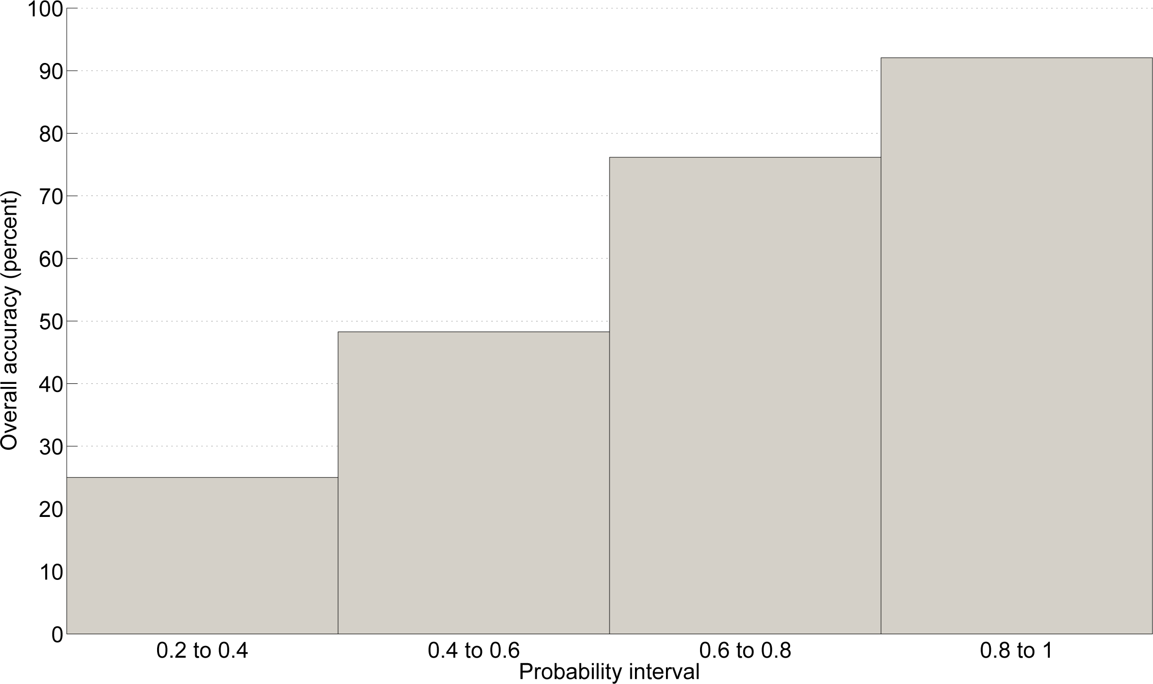
A built-in process to prevent the inappropriate use of existing land cover information as the reference is required in such an automated training sample selection. The a posteriori probability of the classification (which is a classical output of the maximum likelihood classification algorithm) is proposed to determine the scope of the automated training sample extraction method. Similar per-pixel confidence maps are also derived for other classifiers [28]. Low a posteriori probabilities are expected in areas of low consistency between the reference map and the spectral signature distributions. These low values can indicate either that the reference map poorly represents the current land cover or that the classifier cannot discriminate between classes based on the input dataset. This probability allows for the unreliably classified pixels to be masked out and left explicitly undetermined. In this study, the overall accuracy was computed for different levels of a posteriori probability to assess their impact on the confidence in the land cover classification.
4. Validation
Two datasets were used for the validation of the classification outputs. Those datasets were based on random point-based sampling and were independent of the reference dataset used for the training of the classifiers.
Over the South American region, the validation dataset was a subset of a global validation dataset collected by regional experts in the framework of the GlobCover initiative [29]. Those regional experts visually photo-interpreted the sample points, based on a very high resolution image, NDVI annual profiles and their knowledge of the area. For each interpretation, the experts were asked to indicate their level of certainty. Only the points flagged as certain were used in this paper. This dataset is thus highly reliable, but limited to a set of 149 points.
Over Eurasia, the validation dataset is made of a simple random sample of points that were visually interpreted by the authors using the “Bing Map” web service. In total, a set of 700 points was photo-interpreted, from which 43 points have been discarded, because of ambiguity about their actual land cover class (low spatial resolution of the available imagery, remaining clouds or the absence of agreement between the authors).
For each output, the overall accuracy value was computed, estimating the proportion of correctly classified pixels. In addition, an “adjusted accuracy measure” was computed, which tolerates errors with little impact on the description of the landscape [30]. Indeed, due to the high fragmentation level in the area and the discrete nature of the classes defined using LCCS, the boundary between adjacent classes is not always obvious. Typically, these minor errors include confusion between classes that are semantically close. This is the case for the confusion between Classes 30 and 40, which only differ from a cropland dominance point of view (more than 50% cropland in Class 30 and less than 50% in Class 40). The same reasoning can be applied to Classes 100 and 110, which describe combinations of vegetation types with a dominance of either woody or herbaceous vegetation. The other “minor” errors include confusion between mosaic classes and their “pure” dominant component: Classes 10/30, 30/40, 40/60, 40/70, 40/90, 100/90, 100/70, 100/60, 100/110 and 110/130. Confusion between “mixed forests” and “pure forests” were also considered as minor errors: classes 60/90, 70/90. The definition of each class was given in Table 1.
In addition to the quantitative accuracy assessment, a systematic quality control was also recommended to detect macroscopic errors [31] and build confidence in the results. This qualitative validation was based on a systematic descriptive protocol, in which each part of the map was visually examined and its accuracy documented in terms of type of error, landscape pattern, discrepancy between input images and classification results, etc. Macroscopic errors may indeed have little impact on the confusion matrix, but significantly decrease the overall acceptance of a land cover product by users. We focused on omissions of small, yet important, landscape structures (water bodies, urban areas, deforestation patterns, etc.) and the presence of visual artifacts.
5. Results
5.1. Eurasia
In Eurasia, the overall accuracy of the GML was significantly higher than that of the SVM. However, the quantitative difference is quite small, and visual inspection showed two very similar results (Figure 4).
A set of 42 classification results corresponding to six sizes of local windows for the training, three α values for the iterative trimming, three different window sizes for the MBRF and a control without self-cleaning have been obtained, validated and visually checked. These results are only shown for the GML classifier, because of their higher overall accuracy.
The results of the Eurasian test area (Tables 2 and 3) show a significant improvement in the overall accuracies compared with thematic data used as a training reference. The overall accuracy of the GML classification results is indeed between 2.4% and 5.8% better than the overall accuracy of the reference dataset (65.2%). For the adjusted accuracy, the classification results are on average 2.5% better. These two differences are statistically significant with a confidence level of 99%.
Compared with other global products, the resulting map is also better in the study area. Due to the different thematic precision of the products, only the adjusted overall accuracy was relevant. However, these results should still be considered with care because of the matching between the legends. The adjusted overall accuracy of the MODIS product in this study area was 69.1% using the same validation protocol after legend translation. This is mainly due to a poor distinction between croplands and pastures, which represent approximately 80% of the errors. In the case of the GlobCover 2009 product, the adjusted overall accuracy was 62.3%. The main confusion was between grassland and sparse vegetation, and more than 50% of the errors occurred with the mosaic classes.
As expected, the agreement between the training dataset and the classification results decreases when the size of the classification tiles increases. There is indeed a drop of 2% of agreement between the classifications with central tiles of 200-by-200 pixels and compared with those with central tiles of 2000 pixels. However, the quantitative assessment of the classification results using the independent dataset shows that the optimal window size for the training is around 1200 pixels (tiles of 400 pixels). This window size indeed turns out to be the best for all methods in terms of adjusted accuracy and in all, but two, cases for the overall accuracy. Qualitatively, artificial boundaries between tiles are better reduced with this window size, while they are visible for smaller and larger windows. Furthermore, 400-by-400-pixel tiles seem to provide the best compromise between keeping locally important features, such as cities, and adjusting to land cover changes based on information from outside the area that is classified.
Concerning the self-cleaning strategy, MBRF performs better than trimming for the small tiles, even if trimming is interesting in the case of outdated reference data. A combination of the best spatial and spectral filters achieved the same thematic accuracy as the best MBRF. In any case, the overall accuracy decreases when the size of the MBRF increases, but using 3-by-3 or 5-by-5 MBRF improved the classification results compared with the original reference dataset. On the other hand, there is no clear trend due to the change in the trimming parameter in the Eurasia test area. The removal of outliers seems to have a limited impact on the estimation of the distribution parameters of the spectral values within each class.
Despite the small differences in overall accuracies, some important macroscopic changes can be highlighted in Eurasia (Figure 5). Obviously, the spatial resolution of some classes has been improved in the areas where GLC 2000 is used as a reference. Furthermore, the city, mislocated in the reference, is correctly located in the classification results.
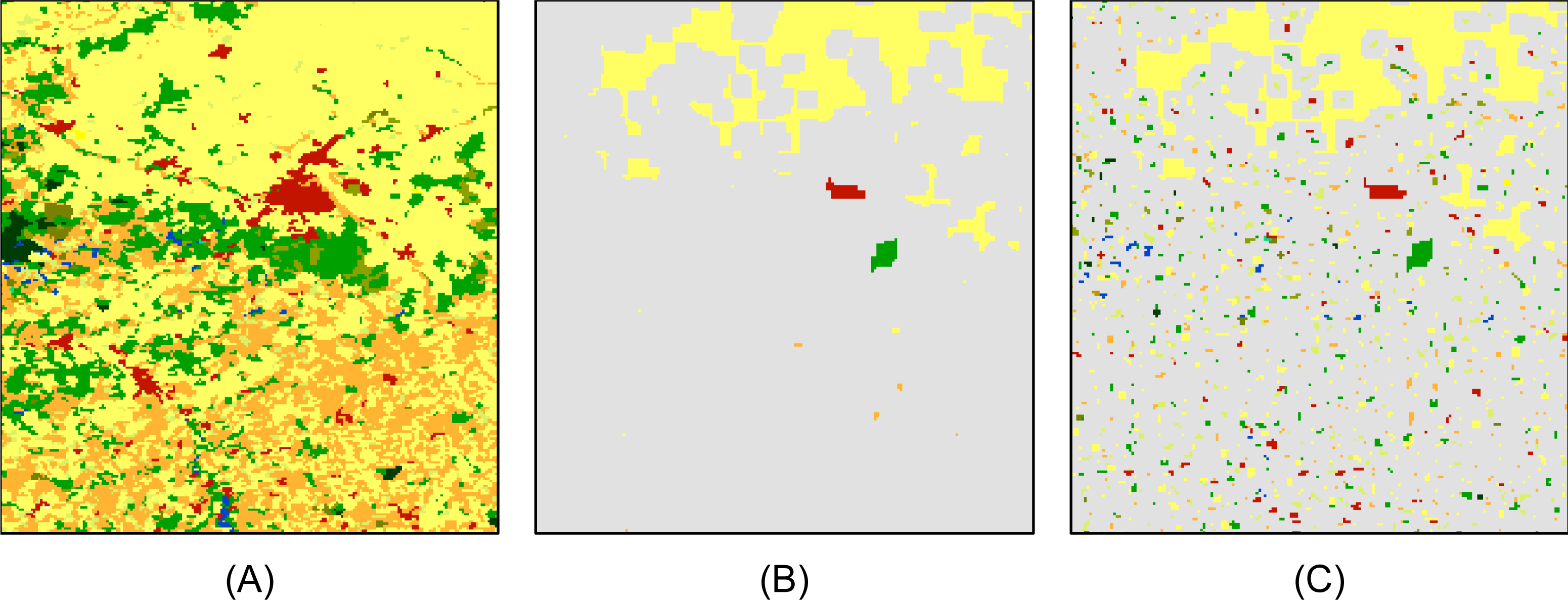
More importantly, the overall accuracy is strongly and positively correlated with the a posteriori probability, as shown in Figure 6. These probabilities appear to be a good indicator of the classification reliability. By thresholding this probability, the most reliable classification results can be selected and the others discarded. In the Eurasian test area, for instance, the overall accuracy of the pixels with a membership probability above 0.6 reaches 85.6%, which is significantly better than the widely accepted 80% target [32] with a 95% confidence level. In terms of coverage, these pixels represent about 70% of the Eurasian region, which is similar to the proportion of the map above 60% confidence in a comparable study in South America [33]. The areas of low probability, colored in grey in Figure 7, should then be processed with alternative classification methods. These are the limits of applicability of the proposed method of automated training sample selection.
The qualitative analysis of the impact of the tile size on the classification results also reveals macroscopic errors that are not highlighted by the overall accuracy. The three main issues are illustrated in Figure 7.
The first example (in black) illustrates a macroscopic change in the landscape due to a natural hazard. The needle-leaved forest in the Western region of the subset was indeed devastated by fire and replaced with broadleaved forest after the reference dataset was completed. This change is not captured by the small training sample window, which, therefore, simply copied the reference inside the forest class.
The second subset (in red) illustrates the need of very local training samples to capture the variability of some land cover classes. The urban areas are the best examples of such variability, as they are composed of a mixture of dense and sparse urban areas together with vegetation. Schneider et al. [34] used “urban ecoregions” to stratify the classification, but the results of the present study suggest that even more local training sets are necessary.
The third case (in green) highlights the presence of artificial boundaries between adjacent processing tiles in classification outputs. As already mentioned, tile boundaries are less present with the 400 tiles than with smaller or larger tiles. These tile features appear where the training samples do not provide enough class separation for the classification, either due to erroneous training data or non-informative spectral data in the images. The artificial tile limits (corresponding to tile boundaries) occurred in areas of low a posteriori probability and could be discarded by applying the a posteriori probability threshold to screen out poor classification outputs.
5.2. South America
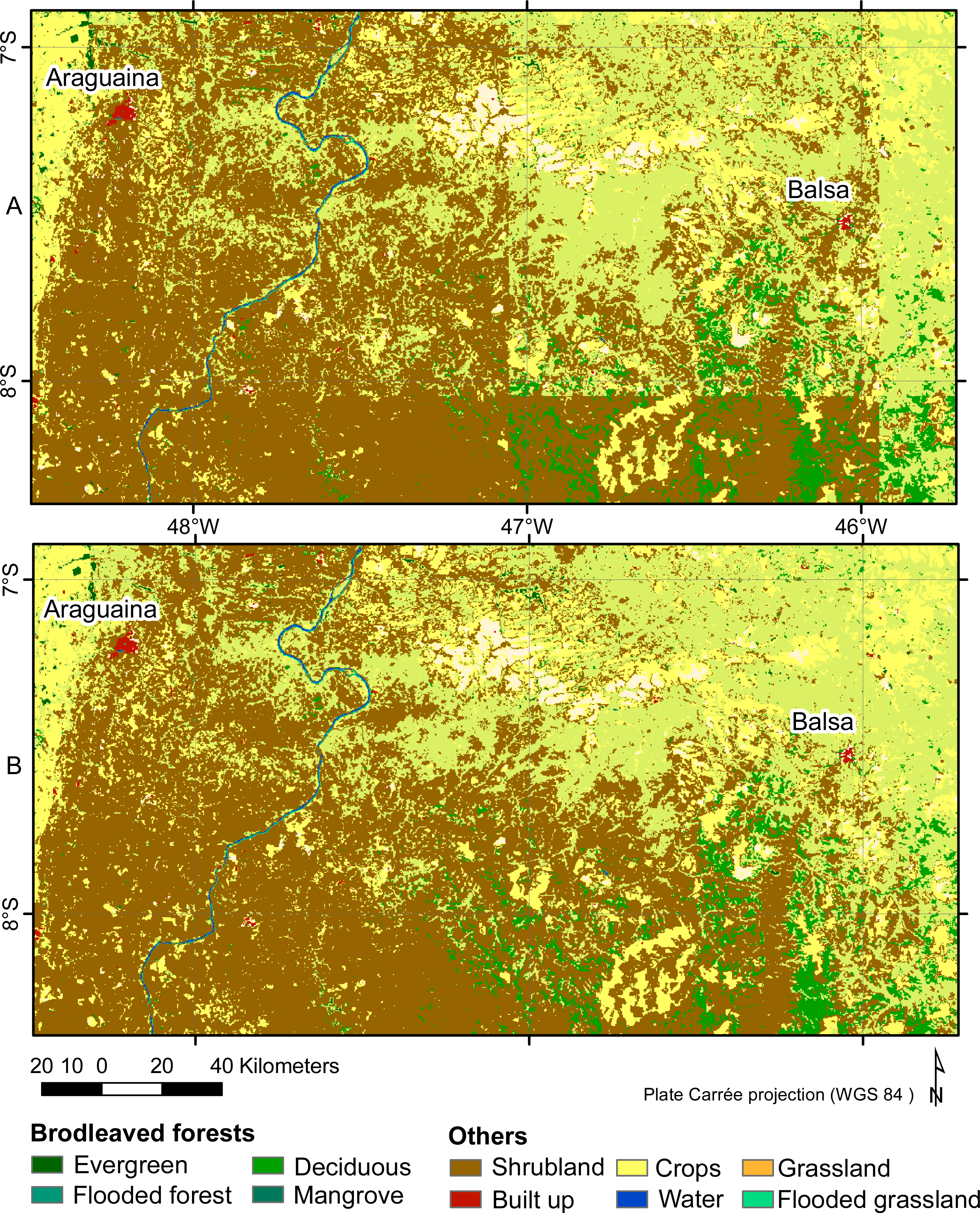
In South America, the overall accuracy of the SVM was one percent lower than for the GML, but this difference was not statistically significant. However, the GML classification outperformed the SVM classification in terms of macroscopic errors. The SVM failed to detect deforested areas when they were under-represented in the training dataset, as shown in Figure 8.
Based on the 149 points photo-interpreted by local experts, the best methods are the trimming with α = 0.05 or 0.1 and the 3-by-3 MBRF. The size of the classification tile has also an impact on the classification results, and the best quantitative results are achieved with a tile size of 400 pixels. The combination between a tile size of 400 pixels and each of the three best methods for sample cleaning achieved an overall accuracy of 91.9%. The differences between the training sample selection methods are however not statistically significant at a confidence level of 90%, but this is probably due to the small sample size. Compared with the overall accuracy of the training dataset (89.2%), the best classification results are significantly higher at a 90% confidence level.
The detection of new patterns of deforestation is found to be accurate. Indeed, 10 out of 10 randomly located points that fell in an area labeled as forest in the reference, but actually deforested in the classification results, were correctly classified as crop. Figure 8 shows that the deforestation, often missing in the reference due to its coarser spatial resolution and the older date, is precisely delineated by the automated classification. The detection of rivers has also been improved thanks to the better spatial resolution of MERIS data.
6. Discussion
This study shows that the automation of the training sample extraction allows capitalizing on the available land cover information. On the one hand, in the two case studies, the thematic accuracy of the new maps is higher than the original reference datasets used for training. On the other hand, the main issue of the proposed approach is its sensitivity to systematic errors in the training dataset. The results showed that this issue can be partly detected based on the low a posteriori probabilities of the classification (which is characteristic of uncertain areas).
The lower quality of the SVM-based results compared with the GML was unexpected, because SVM was found as the most accurate classifier in previous comparative studies [35,36]. However, this can be explained by a combination of unfavorable conditions for the SVM and favorable ones for the GML. On the one hand, there is indeed a large number of classes (22) for an SVM that is originally designed for two-class problems. In addition, SVM is based on extreme values to define its support vectors. Mixed pixels on the edge of the distribution therefore provide useful information [37], but large error rates in the training datasets affect both the learning and the optimization process, even with the soft margin used in this study. On the other hand, the GML could rely on good estimates of the a priori probability of each class, which are not directly available for samples of existing signatures. GML could also take advantage of the large number of training samples to increase the confidence on the parameters of the Gaussian distributions. Finally, the preliminary feature selection is advantageous for GML, knowing that SVM could have managed a larger feature space.
The results show that local training data and a priori probability extraction increase the performance of the maximum likelihood classification over large areas. The same set of parameters has been identified as the best choice for the two contrasting study areas with different training sample precisions and landscape complexities. Because it was also approximatively 20 times faster than SVM training, the local training method with GML was selected to be applied at the global scale. The results were encouraging, but a complementary classification approach still needed to be combined with this first land cover output in the case of low a posteriori probability, in order to improve the overall accuracy. The final product will be freely distributed in the frame of the ESA LC CCI project, after validation by international experts.
The relatively small tile size of the best training configuration highlights the need for locally relevant training samples. Such a need had already been pointed out in previous studies, but rarely at such a small scale factor. These results confirm that the collection of training samples remains a major challenge, especially for global applications, and that the location of these samples is an important factor to take into account during the classification process.
The tile-based processing yields artificial boundaries in areas of low consistency, especially between classes that are distinguished by a single gradient. In a production phase, this problem can be mitigated by increasing the overlap between adjacent tiles, for instance by reducing the size of the tile, but keeping the same area for the training sample selection (Figure 9). However, removing artificial tile boundaries does not solve the spatial consistency problem that is the original source of the artifacts. A combination with other methods therefore remains necessary in those areas in order to achieve higher thematic accuracy.
7. Conclusions
The aim of this study was to evaluate the potential use of training dataset extraction methods from an existing database for global land cover mapping. It showed that the quality of the classification results based on local training set selection and self-cleaning could automatically yield a more accurate map than the original reference dataset and higher thematic accuracy than other global land cover products. The results also suggest that the same set of parameters could be applied globally for optimal results.
Further work is necessary to identify the best add-in methods in regions where the use of existing LC map is not appropriate. The geographic scope of the proposed automated approach is indeed determined by its built-in quality control, which detects largely inconsistent areas between the existing land cover maps and the remote sensing time series.
Acknowledgments
We thank three anonymous reviewers for their valuable comments, which helped to improve this manuscript. This study was funded by the ESA CCI project. The authors thank Olivier Arino, Frank Martin Seifert and Vasileos Kalogirou for their support and valuable comments. We would also like to thank the experts who worked on the independent validation of our product for their valuable input: Valery Gond, Carlo Di Bella and Yosio Edemir Shimabukuro. Last, but not least, we acknowledge the use of the Orfeo Toolbox (OTB) library for implementing our processing chain.
Author Contributions
This study was coordinated by the Pr. Pierre Defourny. Carsten Brockmann was responsible for the radiometric and geometric corrections of the MERIS data. Eric Van Bogaert worked on the compositing algorithm and Sophie Bontemps performed the class separability analysis. Julien Radoux did the sample cleaning and the classification tests. Last but not least, Céline Lamarche manages the quality assessment.
Conflicts of Interest
The authors declare no conflicts of interest.
References
- Hollmann, R.; Merchant, C.; Saunders, R.; Downy, C.; Buchwitz, M.; Cazenave, A.; Chuvieco, E.; Defourny, P.; de Leeuw, G.; Forsberg, R.; et al. The ESA climate change initiative: Satellite data records for essential climate variables. Bull. Am. Meteorol. Soc 2013, 94, 1541–1552. [Google Scholar]
- Herold, M.; Achard, F.; deFries, R.; Mollicone, D. Earth Observation and Political Negotiations: Linking Requirements and Capabilities in the Context of the UNFCCC/REDD Process. Proceedings of the 33rd International Symposium on Remote Sensing of Environment (ISRSE 2009), Stresa, Italy, 4–8 May 2009; pp. 1–4.
- Defries, R.; Townshend, J. NDVI-derived land cover classifications at a global scale. Int. J. Remote Sens 1994, 15, 3567–3586. [Google Scholar]
- DeFries, R.; Hansen, M.; Townshend, J.; Sohlberg, R. Global land cover classifications at 8 km spatial resolution: The use of training data derived from Landsat imagery in decision tree classifiers. Int. J. Remote Sens 1998, 19, 3141–3168. [Google Scholar]
- Loveland, T.; Reed, B.; Brown, J.; Ohlen, D.; Zhu, Z.; Yang, L.; Merchant, J. Development of a global land cover characteristics database and IGBP DISCover from 1 km AVHRR data. Int. J. Remote Sens 2000, 21, 1303–1330. [Google Scholar]
- Arino, O.; Gross, D.; Ranera, F.; Leroy, M.; Bicheron, P.; Brockman, C.; Defourny, P.; Vancutsem, C.; Achard, F.; Durieux, L.; et al. GlobCover: ESA Service for Global Land Cover from MERIS. Proceedings of IEEE International Geoscience and Remote Sensing Symposium (IGARSS 2007), Barcelona, Spain, 23–28 July 2007; pp. 2412–2415.
- Friedl, M.; Sulla-Menashe, D.; Tan, B.; Schneider, A.; Ramankutty, N.; Sibley, A.; Huang, X. MODIS Collection 5 global land cover: Algorithm refinements and characterization of new datasets. Remote Sens. Environ 2010, 114, 168–182. [Google Scholar]
- Bontemps, S.; Arino, O.; Bicheron, P.; Brockmann, C.; Leroy, M.; Vancutsem, C.; Defourny, P. Operational Service Demonstration for Global Land Cover Mapping. In Remote Sensing of Land Use and Land Cover: Principles and Applications, 1st ed; Remote Sensing Applications Series; Giri, C.P., Ed.; CRC Press–Taylor & Francis: Boca Raton, FL, USA, 2012; Chapter 16; pp. 243–264. [Google Scholar]
- Colditz, R.; Schmidt, M.; Conrad, C.; Hansen, M.; Dech, S. Land cover classification with coarse spatial resolution data to derive continuous and discrete maps for complex regions. Remote Sens. Environ 2011, 115, 3264–3275. [Google Scholar]
- Hansen, M.; Defries, R.; Townshend, J.; Sohlberg, R. Global land cover classification at 1 km spatial resolution using a classification tree approach. Int. J. Remote Sens 2000, 21, 1331–1364. [Google Scholar]
- Muchoney, D.; Strahler, A.; Hodges, J.; LoCastro, J. The IGBP DISCover confidence sites and the system for terrestrial ecosystem parameterization: Tools for validating global land-cover data. Photogramm. Eng. Remote Sens 1999, 65, 1061–1067. [Google Scholar]
- Pal, M.; Mather, P. Some issues in the classification of DAIS hyperspectral data. Int. J. Remote Sens 2006, 27, 2895–2916. [Google Scholar]
- Foody, G.; Arora, M. An evaluation of some factors affecting the accuracy of classification by an artificial neural network. Int. J. Remote Sens 1997, 18, 799–810. [Google Scholar]
- Tuia, D.; Pasolli, E.; Emery, W. Using active learning to adapt remote sensing image classifiers. Remote Sens. Environ 2011, 115, 2232–2242. [Google Scholar]
- Brodley, C.E.; Friedl, M.A. Identifying and Eliminating Mislabeled Training Instances. In AAAI; AAAI Press: Menlo Park, CA, USA, 1996; Volume 1, pp. 799–805. [Google Scholar]
- Vancutsem, C.; Bicheron, P.; Cayrol, P.; Defourny, P. An assessment of three candidate compositing methods for global MERIS time series. Can. J. Remote Sens 2007, 33, 492–502. [Google Scholar]
- Di Gregorio, A.; Jansen, L. Land Cover Classification System (LCCS): Classification Concepts And User Manual. In GCP/RAF/287/ITA Africover-East Africa Project and Soil Resources, Management and Conservation Service; Food and Agriculture Organization: Rome, Italy, 2000; pp. 1–91. [Google Scholar]
- Herold, M.; Mayaux, P.; Woodcock, C.; Baccini, A.; Schmullius, C. Some challenges in global land cover mapping: An assessment of agreement and accuracy in existing 1 km datasets. Remote Sens. Environ 2008, 112, 2538–2556. [Google Scholar]
- Bontemps, S.; Bogaert, P.; Titeux, N.; Defourny, P. An object-based change detection method accounting for temporal dependencies in time series with medium to coarse spatial resolution. Remote Sens. Environ 2008, 112, 3181–3191. [Google Scholar]
- Hansen, M.; Loveland, T. A review of large area monitoring of land cover change using Landsat data. Remote Sens. Environ 2012, 122, 66–74. [Google Scholar]
- Vancutsem, C.; Defourny, P. A decision support tool for the optimization of compositing parameters. Int. J. Remote Sens 2008, 30, 41–56. [Google Scholar]
- Bruzzone, L.; Roli, F.; Serpico, S.B. Extension of the Jeffreys-Matusita distance to multiclass cases for feature selection. IEEE Trans. Geosci. Remote Sens 1995, 33, 1318–1321. [Google Scholar]
- Cortes, C.; Vapnik, V. Support vector network. Mach. Learn 1995, 20, 273–297. [Google Scholar]
- Hsu, C.W.; Lin, C.J. A comparison of methods for multi-class support vector machines. IEEE Trans. Neur. Netw 2002, 13, 415–425. [Google Scholar]
- Soille, P. Morphological Image Analysis; Springer-Verlag: Berlin, Germany, 1999. [Google Scholar]
- Desclée, B.; Bogaert, P.; Defourny, P. Forest change detection by statistical object-based method. Remote Sens. Environ 2006, 102, 1–11. [Google Scholar]
- Radoux, J.; Defourny, P. Automated image-to-map discrepancy detection using iterative trimming. Photogramm. Eng. Remote Sens 2010, 76, 173–181. [Google Scholar]
- Colditz, R.; Lopez Saldana, G.; Maeda, P.; Argumedo Espinoza, J.; Meneses Tovar, C.; Victoria Hernandez, A.; Zermeno Benitez, C.; Cruz Lopez, I.; Ressl, R. Generation and analysis of the 2005 land cover map for Mexico using 250 m MODIS data. Remote Sens. Environ 2012, 123, 541–552. [Google Scholar]
- Defourny, P.; Mayaux, P.; Herold, M.; Bontemps, S. Global Land Cover Map Validation Experiences: Toward the Characterisation of Quantitative Uncertainty. In Remote Sensing of Land Use and Land Cover: Principles and Applications, 1st ed.; Remote Sensing Applications Series; Giri, C.P., Ed.; CPC Press-Taylor & Francis: Boca Raton, FL, USA, 2012; Chapter 14; pp. 207–222. [Google Scholar]
- DeFries, R.S.; Chan, J.C.W. Development of a MODIS tree cover validation data set for Western Province, Zambia. Remote Sens. Environ 2002, 74, 503–515. [Google Scholar]
- Mayaux, P.; Eva, H.; Gallego, J.; Strahler, A.; Herold, M.; Agrawal, S.; Naumov, S.; de Miranda, E.; di Bella, C.; Ordoyne, C.; et al. Validation of the global land cover 2000 map. IEEE Trans. Geosci. Remote Sens 2006, 44, 1728–1737. [Google Scholar]
- Strahler, A.H.; Boschetti, L.; Foody, G.M.; Friedl, M.A.; Hansen, M.C.; Herold, M.; Mayaux, P.; Morisette, J.T.; Stehman, S.V.; Woodcock, C.E. Global land cover validation: Recommendations for evaluation and accuracy assessment of global land cover maps. GOFC-GOLD Rep 2006, 25, 1–52. [Google Scholar]
- Blanco, P.; Colditz, R.; Lopez Saldana, G.; Hardtke, L.; Llamas, R.; Mari, N.; Fischer, A.; Caride, C.; Acenolaza, P.; del Valle, H.; et al. A land cover map of Latin America and the Caribbean in the framework of the SERENA project. Remote Sens. Environ 2013, 132, 13–31. [Google Scholar]
- Schneider, A.; Friedl, M.; Potere, D. Mapping global urban areas using MODIS 500-m data: New methods and datasets based on “urban ecoregions”. Remote Sens. Environ 2010, 114, 1733–1746. [Google Scholar]
- Pal, M.; Mather, P. Support vector machines for classification in remote sensing. Int. J. Remote Sens 2005, 26, 1007–1011. [Google Scholar]
- Mountrakis, G.; Im, J.; Ogole, C. Support vector machines in remote sensing: A review. ISPRS J. Photogramm. Remote Sens 2011, 66, 247–259. [Google Scholar]
- Foody, G.; Mathur, A. A relative evaluation of multiclass image classification by support vector machines. IEEE Trans. Geosci. Remote Sens 2004, 42, 1335–1343. [Google Scholar]


| Code | Short Description |
|---|---|
| 10 | Cropland, rainfed |
| 11 | Herbaceous rainfed cropland |
| 12 | Woody rainfed cropland |
| 20 | Cropland, irrigated or post-flooding |
| 30 | Mosaic cropland (>50%)/natural vegetation (tree, shrub, herbaceous) (<50%) |
| 40 | Mosaic natural vegetation (tree, shrub, herbaceous) (>50%)/cropland (<50%) |
| 50 | Tree cover, broadleaved, evergreen, closed to open (>15%) |
| 60 | Tree cover, broadleaved, deciduous, closed to open (>15%) |
| 70 | Tree cover, needle-leaved, evergreen, closed to open (>15%) |
| 80 | Tree cover, needle-leaved, deciduous, closed to open (>15%) |
| 90 | Tree cover, mixed leaf type (broadleaved and needle-leaved) |
| 100 | Mosaic tree and shrub (>50%)/herbaceous cover (<50%) |
| 110 | Mosaic herbaceous cover (>50%)/tree and shrub (<50%) |
| 120 | Shrubland |
| 130 | Grassland |
| 140 | Lichens and mosses |
| 150 | Sparse vegetation (tree, shrub, herbaceous cover) (<15%) |
| 160 | Tree cover, flooded, fresh or brackish water |
| 170 | Tree cover, flooded, saline water |
| 180 | Shrub or herbaceous cover, flooded, fresh/saline/brackish water |
| 190 | Urban areas |
| 200 | Bare areas |
| 210 | Water bodies |
| 220 | Permanent snow and ice |
| 200 | 300 | 400 | 500 | 1000 | 2000 | |
|---|---|---|---|---|---|---|
| Control | 69.3 | 69.5 | 70.0 | 69.5 | 68.0 | 67.6 |
| MBRF 3 × 3 | 71.0 | 70.4 | 70.9 | 70.3 | 69.7 | 69.2 |
| MBRF 5 × 5 | 70.3 | 70.7 | 70.6 | 70.1 | 69.8 | 69.2 |
| MBRF 7 × 7 | 68.9 | 70.1 | 70.0 | 69.8 | 69.5 | 68.6 |
| Trimming 0.05 | 69.3 | 69.5 | 69.8 | 69.8 | 68.6 | 67.5 |
| Trimming 0.10 | 68.7 | 68.7 | 69.3 | 68.9 | 68.4 | 67.8 |
| Trimming 0.20 | 69.2 | 69.3 | 69.7 | 69.2 | 68.1 | 67.6 |
| 200 | 300 | 400 | 500 | 1000 | 2000 | |
|---|---|---|---|---|---|---|
| Control | 81.6 | 80.9 | 82.3 | 81.2 | 79.4 | 78.6 |
| MBRF 3 × 3 | 82.3 | 81.4 | 82.6 | 82.2 | 80.3 | 80.3 |
| MBRF 5 × 5 | 81.4 | 81.2 | 82.8 | 82.0 | 80.8 | 80.2 |
| MBRF 7 × 7 | 80.9 | 81.4 | 82.3 | 81.4 | 80.9 | 79.9 |
| Trimming 0.05 | 81.6 | 81.1 | 82.2 | 80.8 | 79.9 | 78.5 |
| Trimming 0.10 | 80.9 | 80.9 | 81.2 | 80.9 | 79.4 | 78.6 |
| Trimming 0.20 | 81.4 | 80.9 | 81.9 | 80.9 | 79.4 | 78.6 |
© 2014 by the authors; licensee MDPI, Basel, Switzerland This article is an open access article distributed under the terms and conditions of the Creative Commons Attribution license (http://creativecommons.org/licenses/by/3.0/).
Share and Cite
Radoux, J.; Lamarche, C.; Van Bogaert, E.; Bontemps, S.; Brockmann, C.; Defourny, P. Automated Training Sample Extraction for Global Land Cover Mapping. Remote Sens. 2014, 6, 3965-3987. https://doi.org/10.3390/rs6053965
Radoux J, Lamarche C, Van Bogaert E, Bontemps S, Brockmann C, Defourny P. Automated Training Sample Extraction for Global Land Cover Mapping. Remote Sensing. 2014; 6(5):3965-3987. https://doi.org/10.3390/rs6053965
Chicago/Turabian StyleRadoux, Julien, Céline Lamarche, Eric Van Bogaert, Sophie Bontemps, Carsten Brockmann, and Pierre Defourny. 2014. "Automated Training Sample Extraction for Global Land Cover Mapping" Remote Sensing 6, no. 5: 3965-3987. https://doi.org/10.3390/rs6053965