Object-Based Classification of Abandoned Logging Roads under Heavy Canopy Using LiDAR

Abstract
: LiDAR-derived slope models may be used to detect abandoned logging roads in steep forested terrain. An object-based classification approach of abandoned logging road detection was employed in this study. First, a slope model of the study site in Marin County, California was created from a LiDAR derived DEM. Multiresolution segmentation was applied to the slope model and road seed objects were iteratively grown into candidate objects. A road classification accuracy of 86% was achieved using this fully automated procedure and post processing increased this accuracy to 90%. In order to assess the sensitivity of the road classification to LiDAR ground point spacing, the LiDAR ground point cloud was repeatedly thinned by a fraction of 0.5 and the classification procedure was reapplied. The producer’s accuracy of the road classification declined from 79% with a ground point spacing of 0.91 to below 50% with a ground point spacing of 2, indicating the importance of high point density for accurate classification of abandoned logging roads.1. Introduction
In a forested environment, roads can have long-lasting and pervasive impacts on ecosystem health. Forest roads interrupt natural runoff processes and increase overland flow in two ways: soil compaction on road surfaces lowers infiltration rates directly contributing to overland flow [1] and roads act as hydrologic pathways that capture surface and subsurface flow [2]. Increased overland flow typically results in fine sediment production from both surface erosion and road-triggered mass wasting events [3,4]. Furthermore, high forest road densities are associated with an increase in connectivity between sediment sources and streams, leading to higher sediment loads and subsequent water quality problems [5]. Siltation caused by forest roads can be especially damaging to anadromous fish populations [6]. Other impacts of roads on flora and fauna include roads acting as conduits for invasive species [7], decreased tree growth rates [8,9], and reduced near-road habitat suitability for forest-dependent species [10].
Abandoned logging roads, previously used for timber harvest and extraction are found throughout public and private forests within the Pacific Northwest of the United States [11] and in many major forests around the world. These roads may be left unmanaged for years or decades, compounding many typical problems associated with forest roads. Soil disturbance and erosion caused by logging roads is heavily dependent on the method of road construction [12] and many abandoned logging roads were built using poorly considered road building practices [13]. Although the impacts of a new logging road can persist for decades [14,15], road removal treatments have been effective in reducing sediment production from abandoned logging roads [11]. In order to prescribe treatment, forest managers need logging road inventory data to evaluate road impacts. However, maps of logging roads are often unavailable. Remote sensing methods can provide an efficient and reliable way for forest managers to determine if and where abandoned logging roads exist.
While tree cover in forested terrain renders ineffective most traditional remote sensing road detection techniques that rely on aerial photography or satellite imagery, a more recent remote sensing technology, LiDAR (Light Detection and Ranging), is well suited for forest road detection. The distinct advantage of LiDAR is in its capability to poke through small vegetation gaps and collect terrain surface information. Previous authors have used both LiDAR point cloud data and LiDAR-derived raster products to detect and extract forest roads [16,17]. In steep forested terrain, a slope model created from a LiDAR-derived Digital Elevation Model (DEM) has proven especially useful for road detection [17–19]. Since road slopes are generally low, roads in a slope model stand out against the steep grade of the background terrain. The high accuracy of hand-delineated forest roads achieved by White et al. [17] demonstrates the feasibility of using LiDAR derived slope models for road detection. Rieger et al. [18] present a first attempt at automated road extraction under canopy using LiDAR. An edge-enhanced slope model was created from LiDAR data and line features were extracted from the image using an automated “twin snakes” approach. The “snakes” method relies on an energy minimizing function that locks onto nearby edges and can be used to bridge gaps between line segments [20]. This approach has also been applied successfully to registering 2D road vector data to a LiDAR derived DTM [21]. Edge detection methods, such as the “twin snakes” approach are more suited for continuous and intact roads. Since abandoned logging roads tend to be more fractured than maintained forest roads either because of the original road construction method or due to road collapse and erosion that occurred after the road was abandoned, edge detection methods may be less useful when applied to abandoned logging road extraction.
A maximum likelihood classification of LiDAR-derived DEM products in combination with erosion and dilation filters was used by Harmon [22] to successfully classify forest roads under canopy. However, false-positive classifications of road-like features such as streams and gullies, albeit reduced using erosion and dilation filters, were still a significant source of classification error. Also, this pixel-based classification technique had difficulty limiting the classification correctly to road surfaces in low slope areas.
Other authors have attempted to use a combination of LiDAR-derived products and information extracted directly from the LiDAR point cloud for forest road detection. A pixel-based region growing method was used by David et al. [16] to build road pathways from automatically and semi-automatically defined road seeds. Altimetric cross-section profiles were then generated from the LiDAR point cloud to more accurately detect road borders.
A loss of road connectivity caused by road debris and erosion on abandoned logging roads may reduce the effectiveness of pixel-based region growing methods for abandoned logging roads detection. High levels of debris and tree re-growth typically found on abandoned logging roads may also reduce the usefulness of methods that rely on extracting information directly from the LiDAR point cloud. Typically forest road pathways entail an empty volume above the trail surface where vegetation would otherwise be present. Lee et al. [23] present a road detection method that exploits this fact by calculating visibility vectors between road seeds in order to extract forest road pathways. However, using vegetation gaps to infer road locations is less promising for abandoned logging roads where expected gaps are often filled with debris.
Implementing an object-based road classification approach may prove helpful in overcoming some of the previous mentioned challenges to abandoned logging road detection. Object-based classification procedures are typically divided into two stages. Initially, a pixel image is segmented into image objects using a segmentation algorithm. The multiresolution segmentation algorithm, a commonly used segmentation algorithm in object-based image analysis, is a region growing algorithm that combines objects from the pixel-level up, based on a balance of shape and spectral parameters [24]. Objects are grown into adjacent objects if the resulting object minimizes internal heterogeneity. This criterion can be expressed by user-defined weights of spectral reflectance versus shape and the shape weight is further expressed by values of smoothness versus compactness. A scale parameter value constrains resulting object size [25]. Objects may then be classified by taking advantage of both the spectral and spatial qualities of the image objects. For classes that have distinct spatial qualities such as roads and buildings, an object-based approach can be especially useful [26]. Object-based road classification has been successful in classifications using multispectral imagery [27] and, more recently, with the addition of LiDAR derived elevation information [16]. Applications of LiDAR in combination with object-based classification for investigating forest structure and collecting forest inventory data have been especially successful [28]. An object-oriented rule-based classification approach has also been shown to be well-suited for the classification of LiDAR derived surfaces [29].
This paper examines an object-based approach to semi-automatic classification of abandoned logging roads. A LiDAR derived slope model and its edge-enhanced derivative were used as inputs into an initial multiresolution segmentation of road objects. Road seeds and road candidate objects were classified with a rule-based classification and road seeds were grown iteratively into candidate objects. Several post-processing techniques were explored to remove misclassified road-like objects and a pixel-based classification was performed on the slope model for comparison purposes. LiDAR point spacing, or the average ground spacing (in meters) between LiDAR postings, has a strong effect on the vertical error of a LiDAR derived DEM [30]. Furthermore, the usefulness of LiDAR- derived DEMs and their derivatives in capturing forest road information is highly dependent on LiDAR point spacing [17,19,31]. In forested environments, the proportion of LiDAR points that are able to penetrate the canopy and reach the ground surface can be very low. Therefore an examination of the importance of LiDAR point spacing on the effectiveness of road classification was also done by systematically reducing the LiDAR point density (and thus increasing the point spacing) and iteratively running the object-based classification model. An understanding of point density requirements is especially important to forest managers and decision makers who must choose data requirements for flying new LiDAR data in order to detect roads.
2. Study Area and Logging Road Background
2.1. Study Area
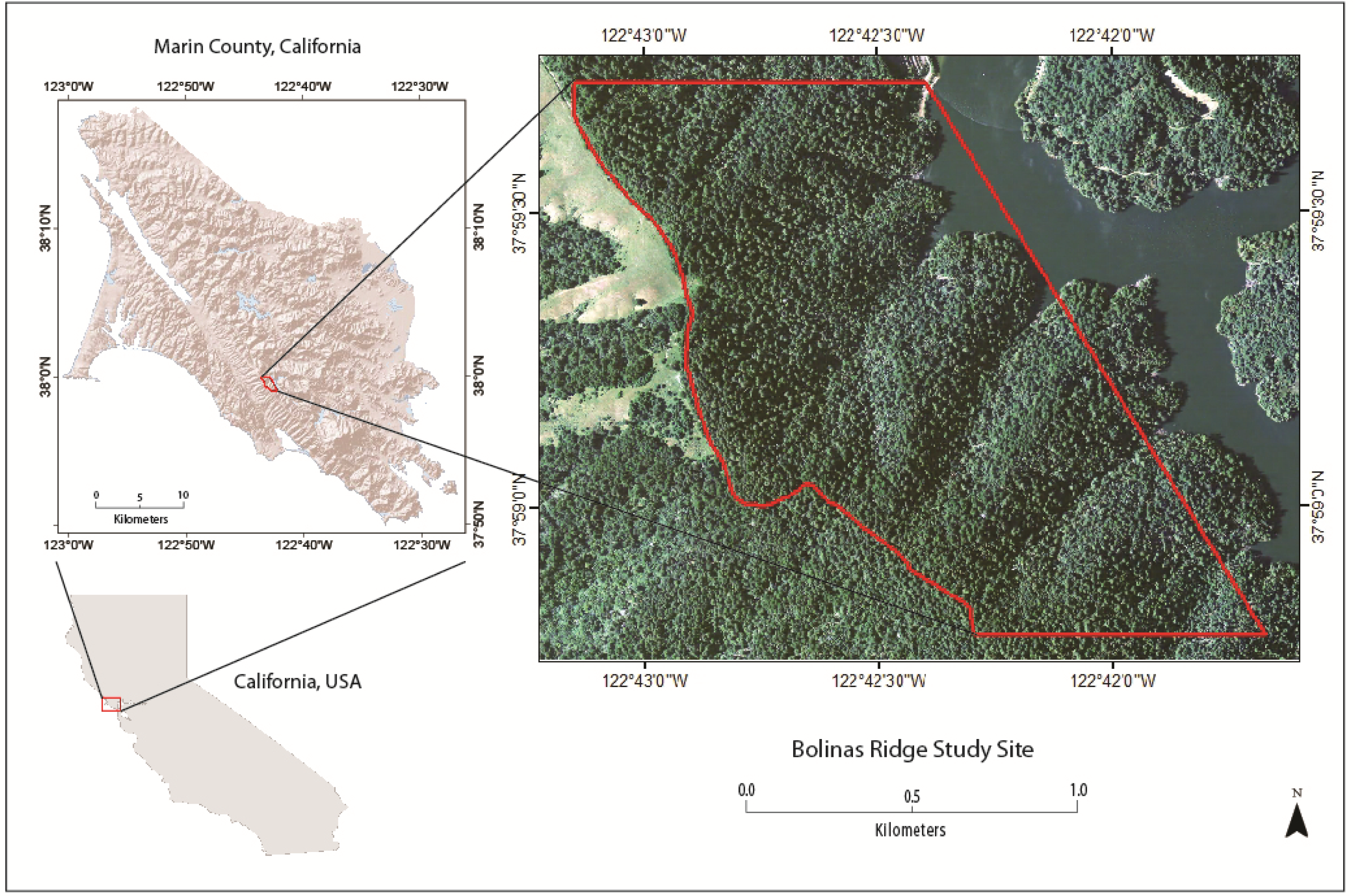
The study area is located on the eastern slope of the Bolinas Ridge above Kent Lake Reservoir in Marin County, California (Figure 1). The site is approximately 3 square kilometers of heavily forested steep terrain, with an average slope of 29° and elevations ranging between 109 and 470 meters above mean sea level. The forest canopy in the study area is primarily characterized by second growth coast redwood and Douglas-fir. Canopy cover is dense and consistent throughout the study site and logging roads within the study site are completely occluded by vegetation (Figure 1).
2.2. Logging Road Background
The Marin Municipal Water District purchased the lands and logging rights for the area containing the study site in 1949 [32]. The extensive network of logging roads found within the study site was likely built shortly after. Between 1949 and 1952 an estimated 3 million board feet of timber was processed at the Ruoff mill, the destination of timber from the study site [32].
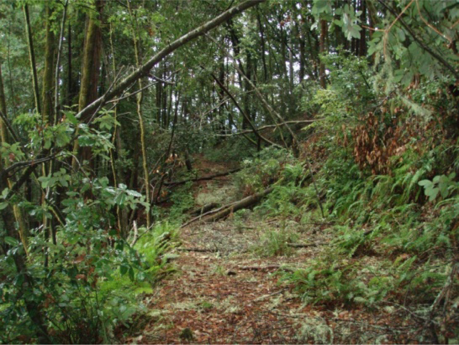
Since logging ended in 1952, logging roads within the study site have remained unmanaged and undisturbed. Bank erosion is evident throughout the road network and fallen trees and forest litter are present on most roads (Figure 2). However, roads are still clearly distinguishable on the ground and little tree growth has occurred on road surfaces. Roads are mostly located perpendicular to the hillslope and following ridgelines. Measured road surface slopes within the study site were found between 0° and 24.5° degrees with an average of 10°. The average road width within the study site was 4.1 meters.
3. Data
LiDAR data acquisition and processing were completed by the National Center for Airborne Laser Mapping (NCALM) as part of the Point Reyes, CA: Landscape Response to Tectonics project. The LiDAR survey was performed with an Optech GEMINI Airborne Laser Terrain Mapper (ALTM) on 8–9 September 2009. The sensor operated at an altitude of 850 meters above ground level, with a pulse rate frequency of 100 kHz, a scan frequency of 40 Hz, and a sampling density of 6 pulses/m2. LiDAR points were classified into ground and non-ground points using TerraSolid’s Terrascan software and point cloud files were tiled into 1 square kilometer blocks.
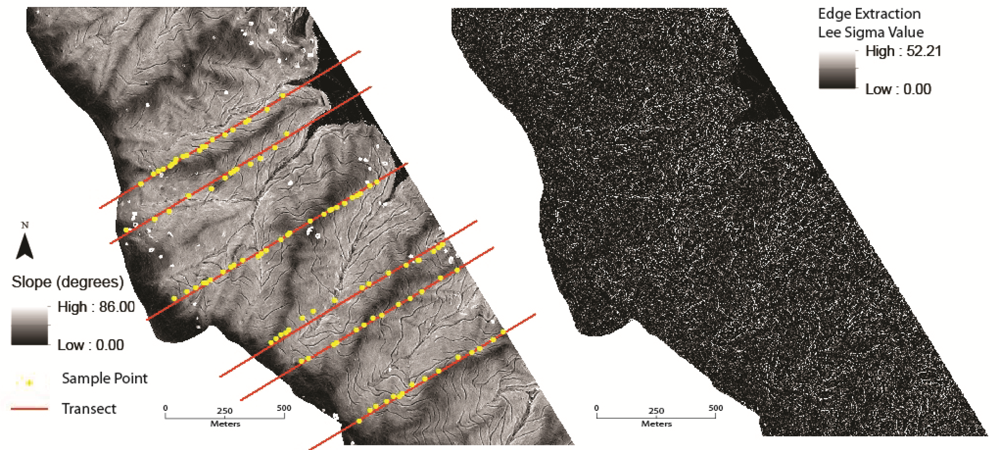
LiDAR ground point data was clipped to the study site boundary and a 1 meter resolution DEM was created in ArcGIS 10.1 using the LAS Dataset to Raster tool. This tool uses a TIN based natural neighbor classification to build a DEM from LiDAR ground points [33]. A slope raster was then created from the DEM using the slope tool in the ArcGIS Spatial Analyst toolset [33]. An examination of the resulting slope model showed a small area with a high concentration of LiDAR artifacts, (distortions in the LiDAR dataset, likely caused by misclassified LiDAR points). The study site dimensions were modified to exclude this area. The slope model shown in Figure 3 represents the slope calculated at a resolution of 1 meter.
4. Methods
4.1. Field Survey
Since logging road maps of the study site were unavailable, a line-intercept field sample was used to gather classification validation points and road characteristics. The field survey was completed over five days between 17 November 2012 and 24 August 2013. Road and non-road points were collected along six transects running from the Bolinas Ridgeline on the western edge of the study site to the eastern edge of the study site. Transect starting points were chosen on the Bolinas Ridgeline in order to cover the entire study site. Originally 200 meter intervals between transects were chosen, but in order to adequately cover the entire study site, it was determined that larger intervals were needed. The exact starting point of each transect was chosen randomly within 100 meter zones. Each transect was then run on a 45 degree angle from the Bolinas ridge trail to the eastern edge of the study site. At each logging road found along a transect, the following road characteristics were collected: width, aspect, slope along road, slope across road, and road position, e.g., within gully, along ridgeline, or following contour. A GPS point was also collected at the center of the road. Non-road GPS points were collected on transects at approximately 100-m intervals to provide non-road validation points. A total of 43 non-road points and 57 road points were collected with a handheld Trimble Juno SB GPS receiver. All GPS points were post-processed with differential correction using reference data from the base provider UNAVCO, Inverness, CA. Despite the stated post-processing accuracy of L1 code of 1–3 m [34], large GPS positional errors can occur in steep forested terrain due to high position dilution of precision (PDOP) and multipath LiDAR returns [35]. A high PDOP indicates that the geometry of the available satellites may lead to positional errors in the resulting GPS points. After a visual inspection of the GPS road points, it became clear that many points were located up to several meters away from their true position. When necessary, GPS road points were moved to the intersection of the corresponding transect and the correct road visually identified on the slope model.
4.2. Object Based Classification
Logging road classification was performed in eCognition® Developer 8.7.2, an Integrated Development Environment (IDE) for image segmentation and the creation of object-oriented classification rule-sets [25]. Within eCognition, an Edge Extraction Lee Sigma filter was first applied to the previously created slope model. This edge extraction algorithm uses an edge filter to create bright and dark edge layers from the original image [25]. In this case dark edges were extracted. A sigma value of 5, determining the strength of the edge detection, was chosen resulting in the image shown in Figure 3. The inclusion of an edge-enhancement filter was precipitated by similar applications by Reiger et al. [18] and Harmon [22]. A sigma value of 5 creates a lee sigma image with strong edge detection.
An initial multiresolution segmentation was performed with the slope image and the edge-enhanced filtered slope image as inputs with equal layer weights. As is often the case with image segmentation in the Ecognition environment, a trial-and-error approach to parameter refinement was needed [36]. In this case the segmentation method, input weights, and shape and compactness parameters were empirically chosen with the goal of creating homogeneous road objects. For this project a scale value of 6 was chosen along with values of 0.1 for shape weight and 0.5 for compactness weight. The shape value of 0.1 gives strong favor to spectral signature over shape during segmentation, while the compactness value of 0.5 indicates equal value was given to maintaining heterogeneity of the “smoothness” and “compactness” of image objects [25]. These parameters were empirically chosen to create the largest possible objects that fall entirely within either a road class or a non-road class.
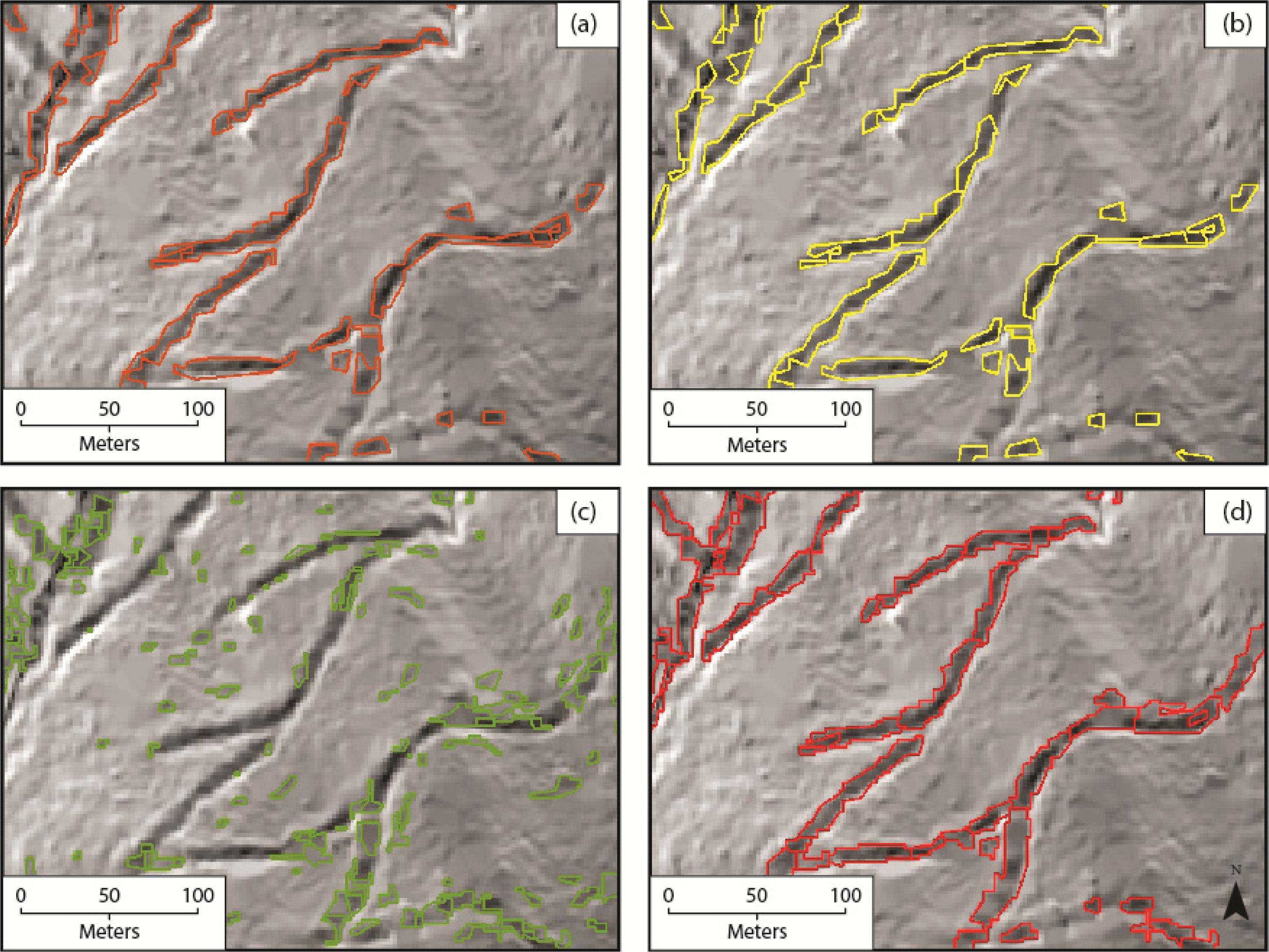
A rule-based classification approach, whereby classification was performed on the image objects based on thresholds for two object parameters, was used to create a road seed class and a road candidate class. The two object parameters selected were the “mean slope value” of an image object and the “mean difference of an object’s slope to its brighter neighbors”. The “mean slope value” parameter is the average slope of each object within the image. The “mean difference of an object’s slope to its brighter neighbors” refers to the mean difference between the mean slope value of each image object and the mean slope value of each adjacent object with a higher mean slope value [25]. More conservative thresholds, meaning a lower “mean value” threshold and higher “mean diffierence to brigher neighbor” threshold, were chosen for the road seed class ensuring a high likelihood that road seed objects were correctly classified (Figure 4a). Remaining unclassified objects were classified into a road candidate class using less conservative parameter thresholds, meaning a higher “mean value” threshold and lower “mean diffierence to brigher neighbor” threshold, in order to ensure most remaining road objects were captured within this class (Figure 4c). Classification parameter thresholds are shown in Table 1.
Road seed objects were merged and small objects below 10 pixels in size were removed from the road seed class. A straightening process was then applied to the road seed class to create straightened elongated road objects more suitable for the road growing. Object straightening was achieved by running multiresolution segmentation iteratively over a reducing scale parameter with a shape criterion of 0.9 and a compactness criterion of 0.9. A comparison of objects before and after straightening is shown in Figure 4a–b.
An iterative road growing and road straightening process was used to grow road seed objects into adjacent road candidate objects. Road seed objects were merged with adjacent road candidate objects based on a decreasing density requirement. Density is a measurement of the distribution of pixels within an object. Denser objects have a structure approaching a square while less dense objects have a shape more similar to a filament [25]. It is expected that as a road increases in length, its density will decrease. Therefore road seed objects were only merged with adjacent road candidate objects if the density of the combined object was less than the density of the road seed object. This process was run iteratively to grow the road into adjacent candidate objects (Figure 4d). Finally, non-road objects fully enclosed by road class objects were classified as roads. The resulting road classification was exported as a shapefile into ArcGIS.
4.3. Road Post Processing
Two levels of post-processing were performed on the results of the object based road classification within ArcGIS 10.1. First, misclassified gullies and streams were removed. A streams layer was created in ArcGIS using the following workflow: LiDAR derived DEM > Flow direction raster > Flow accumulation raster > Streams layer. The resulting stream layer was buffered to 4 meters and used to erase roads falling within natural drainages.
The second post processing level involved hand digitizing ridge roads that were missed by the original object based classification. A plan curvature raster was created from the LiDAR derived DEM using the curvature tool in the Spatial Analyst toolbox [33]. Plan curvature is the rate of change in the flow direction of the surface, following the contour direction. The plan curvature image is helpful in distinguishing ridgelines [37] and ridge roads (Figure 5). Ridge roads visible on the plan curvature image were hand digitized in ArcGIS and joined to the existing classified road layer. Six ridge roads with a total length of 3.9 km were added.
4.4. Unsupervised Pixel-Based Classification
An unsupervised k-means classification of the LiDAR derived slope image was performed to compare with the object-based classification results. Following this approach pixels are separated into a user defined number of clusters based on a minimum distance method [38]. The classification was performed with ERDAS Imagine 2010 with two classes: a road and non-road class.
4.5. LiDAR Point Density Reduction
In order to examine the sensitivity of the road classification to LiDAR point spacing, the original LiDAR point cloud filtered for ground points was thinned at several levels and the previously described slope model creation and object-oriented classification procedures were re-applied. The original LiDAR ground point cloud with a point spacing of 0.91 points per m2 was randomly thinned by a fraction of 0.5. Iterative point thinning resulted in 6 levels of LiDAR ground point spacing (Table 2).
4.6. Classification Accuracy Assessment
Logging road classification accuracy was assessed using GPS ground reference data acquired during the field investigation. Accuracy statistics are summarized in the form of a confusion matrix for each classification result. Classification accuracy assessment was performed for the initial object oriented classification as well as for each post-processing step. Results for the unsupervised classification and for each point spacing level were also calculated.
5. Results
5.1. Object-Based and Pixel-Based Classification Results
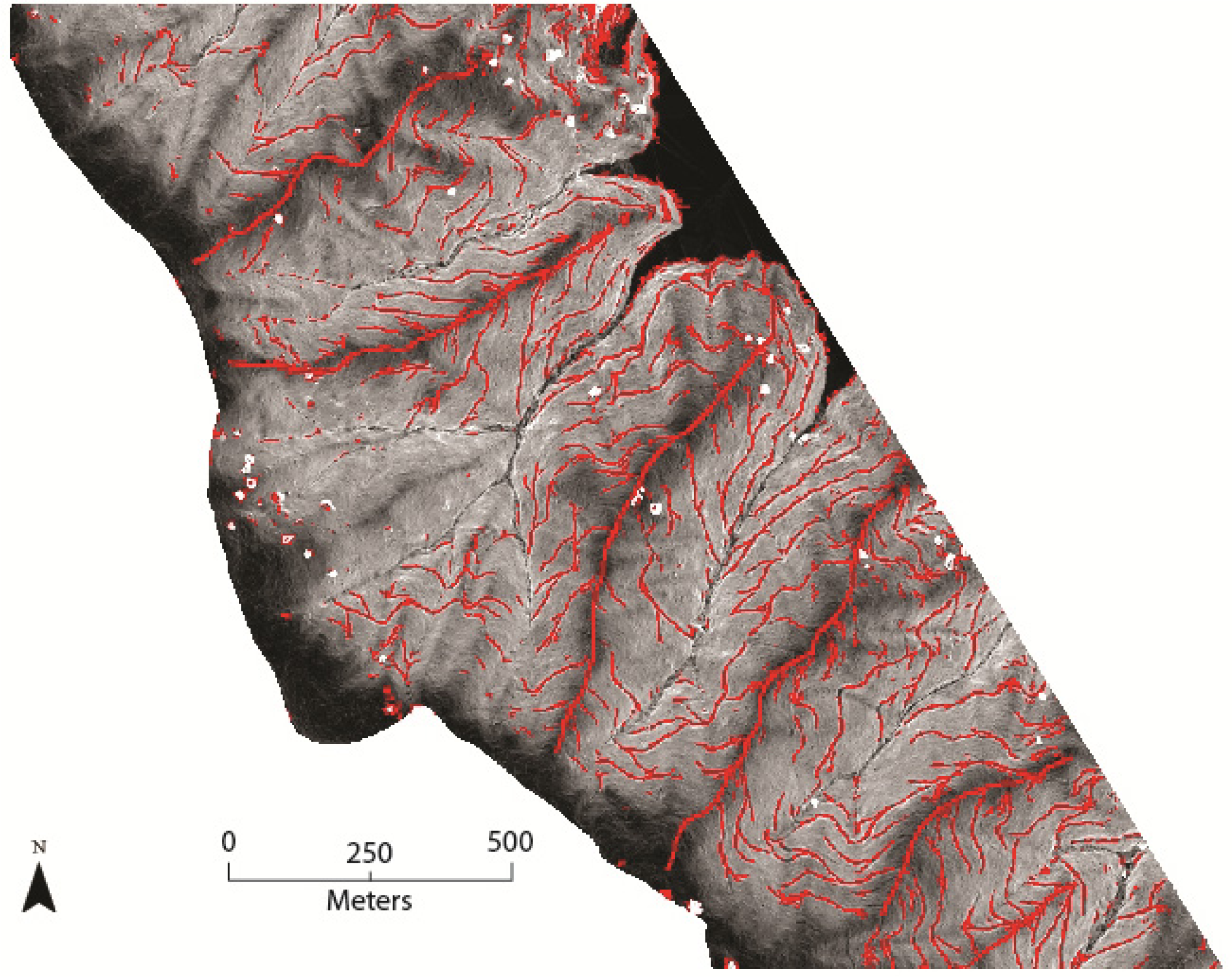
The results for the object-based classification of logging roads summarized in Table 3 show a total accuracy of 86% was obtained from the initial object oriented classification of the LiDAR derived slope image. This accuracy increased to 88% and 90% respectively after extracting misclassified gullies and adding manually digitized ridge roads (Table 3). For the object-oriented classification with gully roads extracted and with ridge roads added, the user’s accuracy was 98% while the producer’s accuracy was only 84%, indicating that a majority of classification errors were errors of omission or roads missed by the classification. Full error matrices are shown in Table 4. A total of 0.275 km2 of area were classified as roads within the study site (Figure 6).
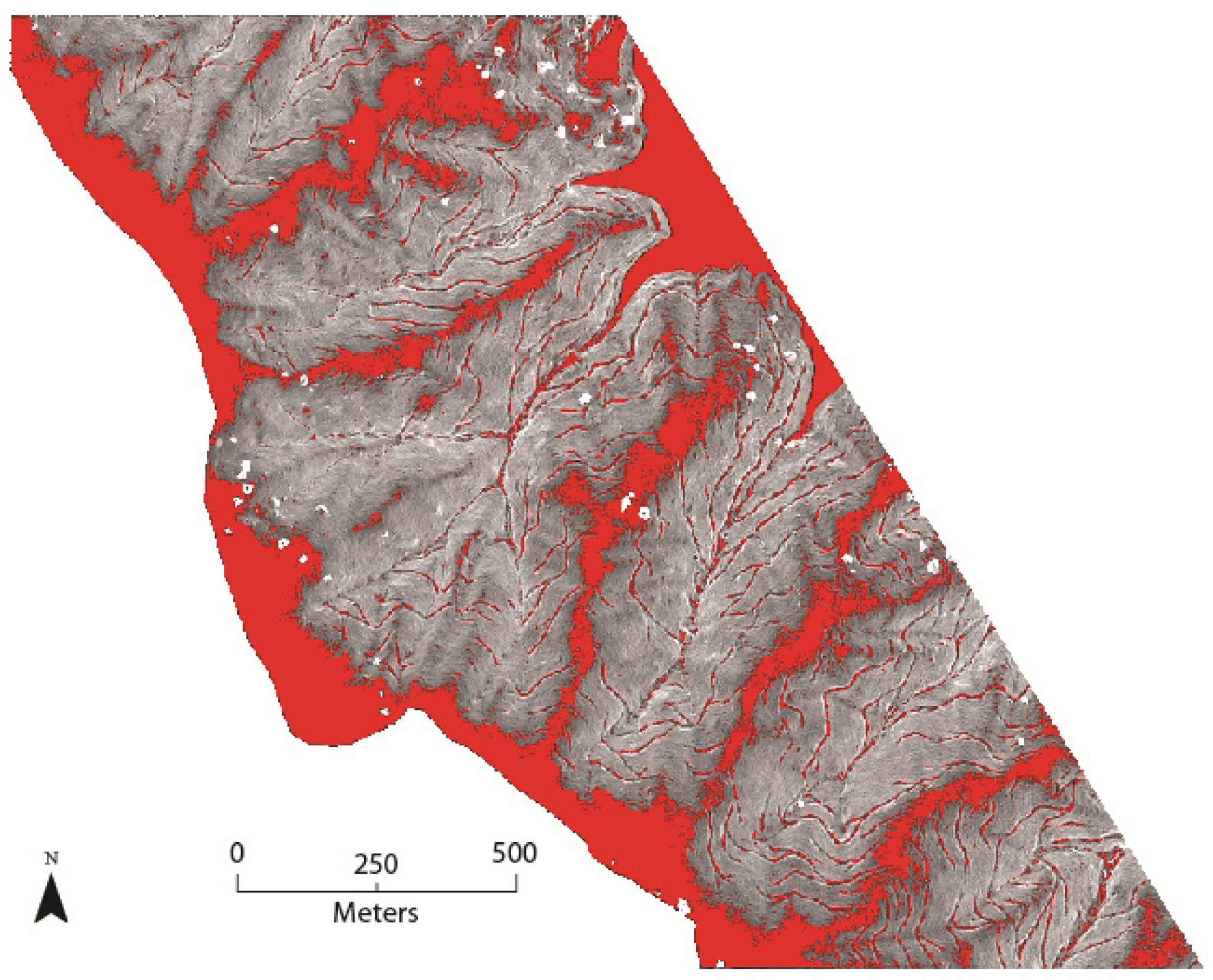
The pixel-based classification results show that the unsupervised classification of logging roads had a total accuracy of 78% (Table 3). A lower user’s accuracy was found in the pixel-based classification than in the object-based classification. Unlike the object-based classification, errors of commission were of significant concern. Errors of commission occurred largely on ridgelines where large areas of low slope were present (Figure 7). The object-based region growing approach was better able to constrain road classification correctly to roads in these areas. Within road areas, the pixel-based classification was less successful in classifying continuous road surfaces. Large and frequent classification gaps are found on the roads in the pixel-based classification results (Figure 7.)
5.2. Point Reduction Classification Results
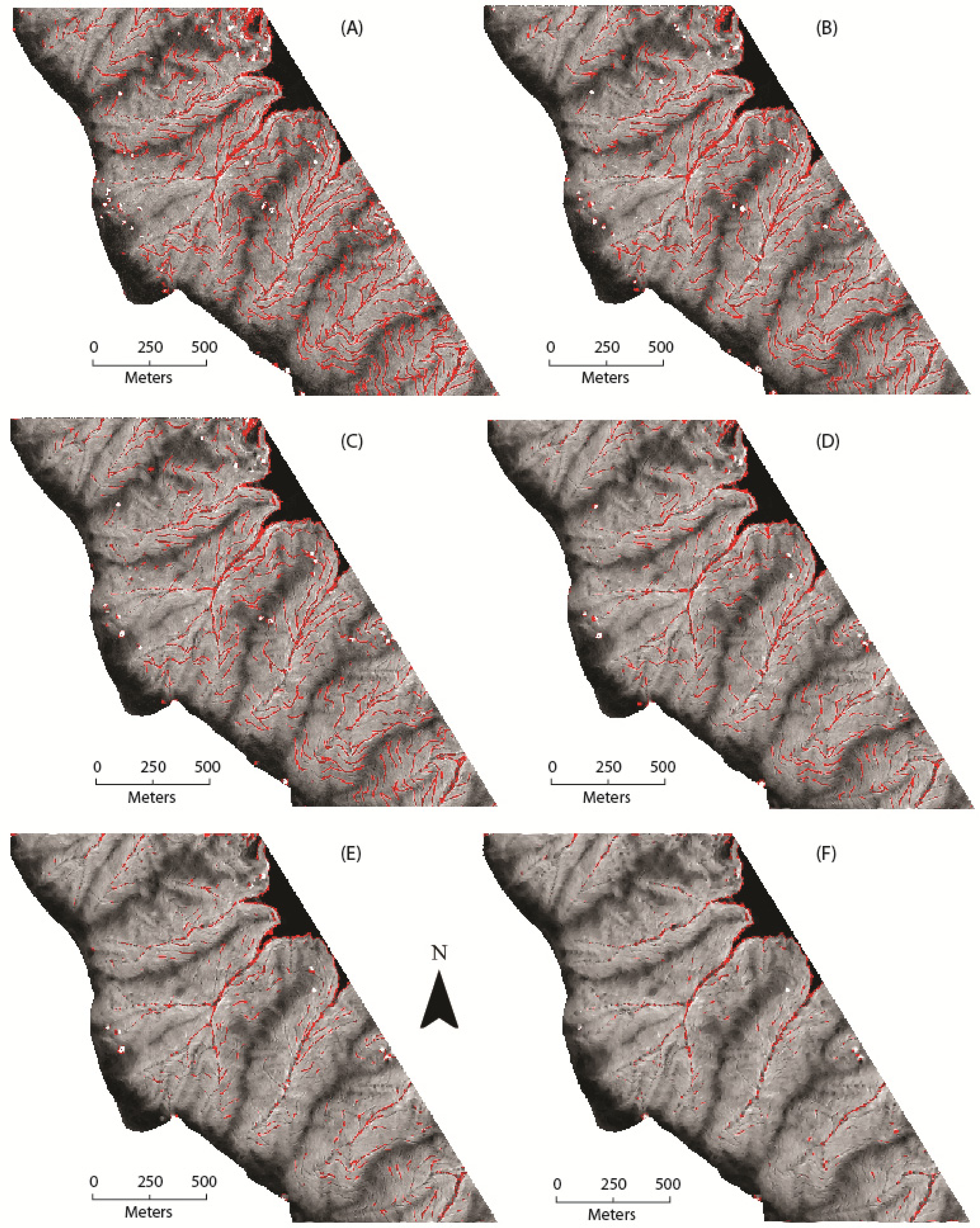
Thinning the LiDAR ground point cloud had a strong impact on the resulting classification accuracy (Table 2). Total accuracy ranged from a high of 86% with a ground point spacing of 0.91 points per m2 to 46% with a ground point spacing of 5.66 (Table 2) when the object-based classification was applied without post-processing. The decline in producer’s accuracy indicates that errors of omission are the cause of reducing classification accuracy. This effect is evident in the classification results shown in Figure 8.
6. Discussion
6.1. Object-Based Classification
The fully automated object-based classification performed well with a total accuracy of 86%. This fully automated object-based approach was an improvement over pixel-based unsupervised classification which resulted in a road classification accuracy of 77%. The object-based approach also outperformed a supervised classification approach to forest road detection attempted by Harmon [22], which yielded a classification accuracy of 73% before post processing. Applying shape conditions to road classification allowed the object based classification to minimize errors of commission in low slope areas. The object-based classification was comparable to total classification accuracies of 85%, 76%, and 74% found by Espinoza et al. [19] for a manual road classification based on visualizing the LiDAR point cloud. Distinguishing natural terraces and drainages from roads was a difficulty shared by several authors [16,19]. This problem derives from the fact that some natural features, like ridgelines, can have similar slope characteristics to manmade road objects. While, in most cases, ridge roads were over-classified [16,19], in our case, a majority of the total error was caused by an under-classification of roads on ridgelines. The road detection parameter “mean difference to brighter neighbors” was largely responsible for reducing the effectiveness of road classification on larger ridgelines. Since slope is fairly uniform surrounding a ridge road, the “mean difference to brighter neighbor” threshold eliminates some ridge roads from the classification. This effect was visible when the “mean difference to brighter neighbor” parameter value was refined using a trial-and-error approach. While adding hand-digitized ridge roads from the plan curvature model requires manual interpretation, it does help to reduce missed ridgeline roads in the classification. A two percent increase in total accuracy after adding hand-digitized roads to the initial object-based classification demonstrates that the plan curvature model is a useful tool in distinguishing ridgeline. However, several ridge roads were still missed, because of difficulties in distinguishing ridge roads from the background terrain. Higher LiDAR point density, allowing for increased slope resolution may help in road detection on ridgelines. Several authors found that incorporating an intensity image in forest road classification methods was helpful [16,23]. However, the high level of debris found on abandoned logging roads would reduce its usefulness for abandoned logging road classification.
Misidentification of natural drainage features as roads was another source of classification error. Because of the lack of field points directly within gullies or streams, the extent of this error was not captured in the error results. However, the simple post-processing step of removing drainages from the road classification seems to largely take care of this problem. Espinoza et al. [19] suggest examining the height profile across a potential road object to determine whether it is a road or a natural drainage. Natural drainages tend to have height profiles with a “V” shape while roads will have a partially flat profile.
6.2. LiDAR Point Reduction
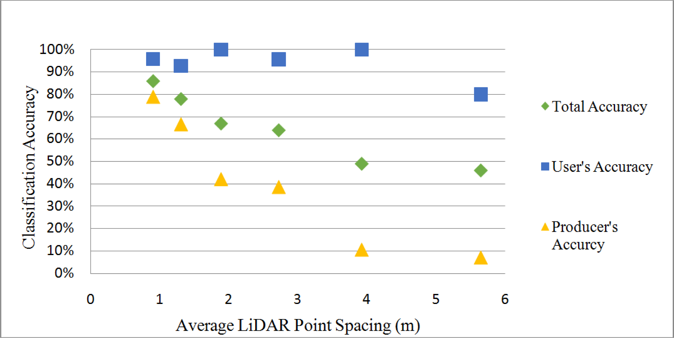
Several authors note that LiDAR ground point densities were greatly reduced under canopy [17,23]. Over 94% of initial LiDAR returns in a study by White et al. [17] were classified as vegetation or other non-ground point returns. By examining the accuracies of manual road classification across several study sites, Espinoza et al. [19] found that point spacing was a large factor in determining classification quality. Our examination of the effects of LiDAR point thinning on the road classification results confirm that finding and reflect a first attempt at isolating the effects of LiDAR point spacing in order to quantify LiDAR point spacing requirements for road detection under canopy. As shown in Figure 8, the usefulness of LiDAR for road detection is drastically reduced as point spacing increases. Between an average ground point spacing of 1 point per m2 and 2 points per m2, producer’s accuracy falls from close to 70 percent to below 50 percent (Figure 9). Within this range, errors of omission reach a level where the usefulness of the resulting classification would be questionable. A similar LiDAR point decimation strategy was performed by [39] to examine the impact of LiDAR post spacing on flood zone delineation. Raber et al. [39] suggest a 4 meter post spacing requirement for flood plain delineation. Our result suggests a much higher LiDAR post spacing is needed for forest road detection.
7. Conclusions
While previous work has looked at the classification of forest roads under canopy, this study is a first attempt at developing methods specifically for the detection and classification of abandoned logging roads. Performing object-based classification on a LiDAR derived slope model of the study site resulted in an initial classification accuracy of 86%, demonstrating the feasibility of a fully automated classification approach. After extracting misclassified drainages and incorporating hand-digitized ridge roads, classification accuracy increased to 90%. Object-based classification proved successful for classifying abandoned logging roads showing considerable road bank erosion and road surface debris and outperformed pixel-based classification attempts in reducing errors of commission.
An assessment of the classification sensitivity to the ground point spacing of the input LiDAR data showed that reasonable classification results were only achievable within a narrow range of LiDAR ground point spacing. This data can be used by forest managers or researchers as a starting point for determining LiDAR point spacing requirements when collecting LiDAR data for the detection of forest roads. Further research looking at the influence of vegetation type and landscape slope characteristics on LiDAR point spacing requirements would also be useful.
Higher LiDAR point densities may further improve the classification accuracies achieved in this study, especially for ridgeline roads. Incorporating other LiDAR products, as inputs for the object-based classification, such as the plan curvature model, could lead to a high accuracy fully automated road classification procedure. Although road debris and forest regrowth pose difficulties when using LiDAR point cloud data for abandoned logging road detection, incorporating the LiDAR point cloud may still prove helpful. With high point densities, forest road debris could be visualized and used as an attribute for logging road detection.
Acknowledgments
The authors would like to thank Nicholas Salcedo and Jason Hoorn for their help in locating the study area and providing useful local knowledge. Thank you, also, to Nathan Greig, Dariya Draganova, and Garrett Bradford for their hard work as field assistants.
Author Contributions
Jason Sherba helped to develop the original research methods for the study and located an appropriate LiDAR dataset. He performed the field study, with the help of his field crew, and the road detection and LiDAR point thinning procedures. He also performed the accuracy assessment of the road detection and analysis of the results. Jason wrote the first draft of the article, including all figures and tables, as well as subsequent drafts working with his coauthors.
Jerry Davis helped develop the original design of the research, worked with the lead author in exploring relevant literature, and suggested the field site to be used to test the method. He planned and participated in the initial field reconnaissance, bringing in local expertise from the Marin Municipal Water District (Nicholas Salcedo) and Stetson Engineering (Jason Hoorn, formerly of Pacific Watershed Associates), then helped design an appropriate field data collection protocol, and provided the appropriate field equipment. During the writing phase and preparation for submission, he helped edit each draft of the text and figures.
Leonhard Blesius helped develop the research topic and methodology based on discussions with National Park Service employees at Point Reyes for whom the subject is of high priority. He also worked with Jason Sherba on the relevant issues of remote sensing in general and object-oriented image analysis specifically. He edited the written document at various draft stages, including text, figures, and literature content.
Conflicts of Interest
The authors declare no conflict of interest.
References and Notes
- Johnson, M.G.; Beschta, R.L. Logging, infiltration capacity, and surface erodibility in western oregon. J. For 1980, 78, 334–337. [Google Scholar]
- Wemple, B.C.; Swanson, F.J.; Jones, J.A. Forest roads and geomorphic process interactions, cascade range, oregon. Earth Surface Process. Landf 2001, 26, 191–204. [Google Scholar]
- MacDonald, L.H.; Coe, D.B. Road sediment production and delivery: Processes and management. Proceedings of the First World Landslide Forum, International Programme on Landslides and International Strategy for Disaster Reduction, Tokyo, Japan, 18–21 November 2008; pp. 381–384.
- Reid, L.M.; Dunne, T. Sediment production from forest road surfaces. Water Resour. Res 1984, 20, 1753–1761. [Google Scholar]
- Wemple, B.C.; Jones, J.A.; Grant, G.E. Channel network extension by logging roads in two basins, western cascades, oregon. Water Resour. Bull 1996, 32, 1195–1207. [Google Scholar]
- Cederholm, C.; Reid, L.; Salo, E.O. Cumulative effects of logging road sediment on salmonid populations in the clearwater river, jefferson county, washington. Proceedings of the Conference Salmon-Spawning Gravel: A Renewable Resource in the Pacific Northwest, Seattle, WA, USA, 6–7 October 1980; pp. 39–74.
- Gelbard, J.L.; Belnap, J. Roads as conduits for exotic plant invasions in a semiarid landscape. Conserv. Biol 2003, 17, 420–432. [Google Scholar]
- Guariguata, M.R.; Dupuy, J.M. Forest regeneration in abandoned logging roads in lowland costa rica1. Biotropica 1997, 29, 15–28. [Google Scholar]
- Rab, M. Recovery of soil physical properties from compaction and soil profile disturbance caused by logging of native forest in victorian central highlands, australia. For. Ecol. Manag 2004, 191, 329–340. [Google Scholar]
- Semlitsch, R.D.; Ryan, T.J.; Hamed, K.; Chatfield, M.; Drehman, B.; Pekarek, N.; Spath, M.; Watland, A. Salamander abundance along road edges and within abandoned logging roads in appalachian forests. Conserv. Biol 2007, 21, 159–167. [Google Scholar]
- Madej, M.A. Erosion and sediment delivery following removal of forest roads. Earth Surf. Process. Landf 2001, 26, 175–190. [Google Scholar]
- Megahan, W.F.; Kidd, W. Effects of logging and logging roads on erosion and sediment deposition from steep terrain. J. For 1972, 70, 136–141. [Google Scholar]
- Appelboom, T.; Chescheir, G.; Skaggs, R.; Hesterberg, D. Management practices for sediment reduction from forest roads in the coastal plains. Trans. ASAE 2002, 45, 337–344. [Google Scholar]
- Croke, J.; Hairsine, P.; Fogarty, P. Soil recovery from track construction and harvesting changes in surface infiltration, erosion and delivery rates with time. For. Ecol. Manag 2001, 143, 3–12. [Google Scholar]
- Ziegler, A.D.; Negishi, J.N.; Sidle, R.C.; Gomi, T.; Noguchi, S.; Nik, A.R. Persistence of road runoff generation in a logged catchment in peninsular malaysia. Earth Surf. Process. Landf 2007, 32, 1947–1970. [Google Scholar]
- David, N.; Mallet, C.; Pons, T.; Chauve, A.; Bretar, F.; Cemagref Montpellier, F. Pathway detection and geometrical description from als data in forested mountaneous area. Int. Arch. Photogramm. Remote Sens. Spat. Inf. Sci 2009, 38, 242–247. [Google Scholar]
- White, R.A.; Dietterick, B.C.; Mastin, T.; Strohman, R. Forest roads mapped using lidar in steep forested terrain. Remote Sens 2010, 2, 1120–1141. [Google Scholar]
- Rieger, W.; Kerschner, M.; Reiter, T.; Rottensteiner, F. Roads and buildings from laser scanner data within a forest enterprise. Int. Arch. Photogramm. Remote Sens. Spat. Inf. Sci 1999. Available online: http://www.isprs.org/proceedings/XXXII/3-W14/pdf/p185.pdf (accessed on 24 April 2014). [Google Scholar]
- Espinoza, F. Identifying Roads and Trails Hidden under Canopy Using Lidar. Master’s Thesis, Naval Postgraduate School, Monterey, CA, USA. 2007. [Google Scholar]
- Kass, M.; Witkin, A.; Terzopoulos, D. Snakes: Active contour models. Int. J. Comput. Vis 1988, 1, 321–331. [Google Scholar]
- Göpfert, J.; Rottensteiner, F.; Heipke, C. Using snakes for the registration of topographic road database objects to als features. ISPRS J. Photogramm. Remote Sens 2011, 66, 858–871. [Google Scholar]
- Harmon, C.F., III. Automating Identification of Roads and Trails under Canopy Using Lidar. Master’s Thesis, Naval Postgraduate School, Monterey, CA, USA. 2011. [Google Scholar]
- Lee, H.; Slatton, K.C.; Jhee, H. Detecting forest trails occluded by dense canopies using alsm data. Proceedings of 2005 IEEE International Geoscience and Remote Sensing Symposium, Seoul, Korea, 25–29 July 2005; pp. 3587–3590.
- Benz, U.C.; Hofmann, P.; Willhauck, G.; Lingenfelder, I.; Heynen, M. Multi-resolution, object-oriented fuzzy analysis of remote sensing data for gis-ready information. ISPRS J. Photogramm. Remote Sens 2004, 58, 239–258. [Google Scholar]
- Definiens, A. Definiens Developer 7—User Guide, 2007. Available online: http://ecognition.cc/download/userguide.pdf (accessed on 24 April 2014).
- Priestnall, G.; Hatcher, M.; Morton, R.; Wallace, S.; Ley, R. A framework for automated extraction and classification of linear networks. Photogramm. Eng. Remote Sens 2004, 70, 1373–1382. [Google Scholar]
- Chen, Y.H.; Su, W.; Li, J.; Sun, Z.P. Hierarchical object oriented classification using very high resolution imagery and lidar data over urban areas. Adv. Space Res 2009, 43, 1101–1110. [Google Scholar]
- Maier, B.; Tiede, D.; Dorren, L. Characterising mountain forest structure using landscape metrics on lidar-based canopy surface models. In Object-Based Image Analysis; Springer: New York, NY, USA, 2008; pp. 625–643. [Google Scholar]
- Brennan, R.; Webster, T. Object-oriented land cover classification of lidar-derived surfaces. Can. J. Remote Sens 2006, 32, 162–172. [Google Scholar]
- Hodgson, M.E.; Bresnahan, P. Accuracy of airborne lidar-derived elevation: Empirical assessment and error budget. Photogramm. Eng. Remote Sens 2004, 70, 331–340. [Google Scholar]
- Krougios, P. Extracting Hidden Trails and Roads under Canopy Using Lidar. Master’s Thesis, Naval Postgraduate School, Monterey, CA, USA. 2008. [Google Scholar]
- Henry, A. Logging-marin’s first industry. Marin Independent Journal 1950. [Google Scholar]
- ArcGIS, E. 10.1 Desktop Help, Available online: http://resources.arcgis.com/en/help/main/10.1/index.html#//00qn0000001p000000 (accessed on 24 April 2014).
- Trimble Navigation Limited, Data Sheet: Juno SB Handheld; Trimble Natigation Limited: Sunnyvale, CA, USA, 2012.
- Deckert, C.; Bolstad, P.V. Forest canopy, terrain, and distance effects on global positioning system point accuracy. Photogramm. Eng. Remote Sens 1996, 62, 317–321. [Google Scholar]
- Myint, S.W.; Gober, P.; Brazel, A.; Grossman-Clarke, S.; Weng, Q. Per-pixel vs. Object-based classification of urban land cover extraction using high spatial resolution imagery. Remote Sens. Environ 2011, 115, 1145–1161. [Google Scholar]
- Peckham, S.D. Profile, plan and streamline curvature: A simple derivation and applications. Proceedings of Geomorphometry 2011, Redlands, CA, USA, 7 September 2011; pp. 27–30.
- Jain, A.K.; Murty, M.N.; Flynn, P.J. Data clustering: A review. ACM Comput. Surv 1999, 31, 264–323. [Google Scholar]
- Raber, G.T.; Jensen, J.R.; Hodgson, M.E.; Tullis, J.A.; Davis, B.A.; Berglund, J. Impact of lidar nominal post-spacing on dem accuracy and flood zone delineation. Photogramm. Eng. Remote Sens 2007, 73, 793–804. [Google Scholar]


| Mean Value | Mean Difference to Brighter Neighbor | |
|---|---|---|
| Road Seed | ≤34 | ≥9 |
| Road Candidate | ≤35 | ≥5 |
| LiDAR Point Spacing | User’s Accuracy | Producer’s Accuracy | Total Accuracy |
|---|---|---|---|
| 0.91 | 0.96 | 0.79 | 0.86 |
| 1.31 | 1 | 0.66 | 0.78 |
| 1.89 | 1 | 0.42 | 0.67 |
| 2.73 | 0.96 | 0.39 | 0.64 |
| 3.93 | 1 | 0.105 | 0.49 |
| 5.66 | 0.8 | 0.07 | 0.46 |
| User’s Accuracy | Producer’s Accuracy | Total Accuracy | |
|---|---|---|---|
| Initial classification | 0.96 | 0.79 | 0.86 |
| Drainages excluded | 1 | 0.79 | 0.88 |
| Drainages excluded/ridge roads added | 0.98 | 0.84 | 0.9 |
| Pixel-based classification | 0.8 | 0.79 | 0.78 |
| (A) | Ground Truth | Total Classified | ||
| Road | NonRoad | |||
| Classification | Road | 45 | 2 | 47 |
| NonRoad | 12 | 41 | 53 | |
| Total Ground Truth | 57 | 43 | 100 | |
| (B) | Ground Truth | Total Classified | ||
| Road | NonRoad | |||
| Classification | Road | 45 | 0 | 45 |
| NonRoad | 12 | 43 | 55 | |
| Total Ground Truth | 57 | 43 | 100 | |
| (C) | Ground Truth | Total Classified | ||
| Road | NonRoad | |||
| Classification | Road | 48 | 1 | 49 |
| NonRoad | 9 | 42 | 51 | |
| Total Ground Truth | 57 | 43 | 100 | |
| (D) | Ground Truth | Total Classified | ||
| Road | NonRoad | |||
| Classification | Road | 45 | 11 | 56 |
| NonRoad | 12 | 35 | 47 | |
| Total Ground Truth | 57 | 46 | 103 | |
© 2014 by the authors; licensee MDPI, Basel, Switzerland This article is an open access article distributed under the terms and conditions of the Creative Commons Attribution license (http://creativecommons.org/licenses/by/3.0/).
Share and Cite
Sherba, J.; Blesius, L.; Davis, J. Object-Based Classification of Abandoned Logging Roads under Heavy Canopy Using LiDAR. Remote Sens. 2014, 6, 4043-4060. https://doi.org/10.3390/rs6054043
Sherba J, Blesius L, Davis J. Object-Based Classification of Abandoned Logging Roads under Heavy Canopy Using LiDAR. Remote Sensing. 2014; 6(5):4043-4060. https://doi.org/10.3390/rs6054043
Chicago/Turabian StyleSherba, Jason, Leonhard Blesius, and Jerry Davis. 2014. "Object-Based Classification of Abandoned Logging Roads under Heavy Canopy Using LiDAR" Remote Sensing 6, no. 5: 4043-4060. https://doi.org/10.3390/rs6054043