Forest Fire Severity Assessment Using ALS Data in a Mediterranean Environment


Abstract
: Mediterranean pine forests in Spain experience wildland fire events with different frequencies, intensities, and severities which result in diverse socio-ecological consequences. In order to predict fire severity, spectral indices derived from remotely sensed images have been used extensively. Such spectral indices are usually used in combination with ground sampling to relate detected radiometric changes to actual fire effects. However, the potential of the tridimensional information captured by Airborne Laser Scanners (ALS) to severity mapping has been less explored. With the objective of addressing this question, in this paper, explanatory variables extracted from ALS point clouds are related to field estimations of the Composite Burn Index collected in four fires located in Aragón (Spain). Logistic regression models were developed and statistically tested and validated to map fire severity with up to 85.5% accuracy. The canopy relief ratio and the percentage of all returns above one meter height were the most significant variables and were therefore used to create a continuous map of severity levels.1. Introduction
Fire is a global phenomenon [1] with 200–500 million hectares being burned annually [2]. Fires affect large areas in a variety of biomes from tropical to boreal being more widespread than any other natural disturbance [2,3]. In some ecosystems, e.g., savannas and grasslands, fire plays an ecologically significant role in biogeochemical cycles and disturbance dynamics. In other ecosystems, fire may lead to the destruction of forests or to long-term site degradation.
In Mediterranean Europe, fire is a major hazard with an average of 45,000 fires being recorded yearly [4]. Therefore, fire constitutes one of the main factors determining the current forest landscape [5], with summertime wildfires causing extensive ecological and economic losses [6] over hundreds of thousands of hectares of forests, shrub lands and grasslands. In Spain, although the last decade, 2001–2010, has seen a reduction in the number of fire incidents (averaging 17.127 per year), the occurrence of large fires (>100 ha) increased. In 2012, 64% of the total area affected by fires was burned in a large fire [7]. Even though Mediterranean species are adapted to natural fire regimes, changes in land use and the cumulative effects of anthropogenic disturbances make vegetation communities more vulnerable to high-intensity wildfires. In addition, climate change forecasts imply an increasing vulnerability of our forests to large-scale fires in the future [8]. In response, scientists and fire managers require the most accurate information available regarding the impact of fire on the environment. The way fire is distributed throughout the affected area is essential for short-term mitigation and restoration treatments, as well as for vegetation recovery monitoring, wildlife studies, soil and hydrologic changes, as well as various ecological processes [9].
In most cases, fire severity and burn severity are used interchangeably to describe fire effects on ecosystems in terms of biophysical alteration (e.g., blackening or scorching of tree-leaves, amount of fuel consumed, depth of burn, soil exposure, etc.). However, these two terms may imply different meanings. Fire severity can be defined as a measure of the immediate fire impact on the environment such as tree mortality and the loss of biomass in the forms of vegetation and soil organic material, while burn severity can be defined as the degree of ecological change caused by fire [9,10]. The Composite Burn Index (CBI) was developed by Key and Benson [11] within the framework of the Fire Effects Monitoring and Inventory Protocol (FIREMON) project for pine forests in western USA, to sample these changes and to summarize the general effects of a fire at a given plot. The CBI has been used and adjusted [9] to a wide range of environments, from Mediterranean to boreal [12–19].
Extensive field surveys are often costly and labor intensive, making the use of remotely sensed data indispensable for fire severity analysis. The removal of vegetation, the exposure of soil, and changes in soil and vegetation moisture content as a result of differences in burn severity, imply changes in the near and short-wave infrared regions of the electromagnetic spectrum that can be detected by multispectral remote sensing devices. Remote sensing products are not only more cost-effective when compared to ground-based methods, but also provide information even in inaccessible areas shortly after fire events [9].
The estimation of burn severity from satellite data has been accomplished using per band reflectance or vegetation spectral indices derived from optical sensors of different spatial resolutions, from 1 km (e.g., Advanced Very High Resolution Radiometer—AVHRR) down to 2 m (e.g., QuickBird), with Landsat satellite images (30 m pixel) being the most commonly used [20]. However, estimations from passive satellite sensors are less sensitive to changes in forest structure [21] than active sensors, such as Radio Detection and Ranging (radar) [22,23] and Airborne Laser Scanner (ALS) [24].
ALS has already been adopted and accepted as a valuable tool in forestry applications due to the three-dimensional nature of the data. The laser pulse penetration characteristics and the multi-return recording capabilities enable an accurate geometry-related approach in forestry, and by extension in wildland fire management [25]. Research focused on this technology has moved from validation of ALS measurement effectiveness for forest studies (e.g., [26,27]), to estimation of continuous variables such as basal area and biomass (e.g., [28,29]), as well as to forest structure analysis over large areas (e.g., [30–33]) and the quantification and assessment of canopy gaps and patches within forests (e.g., [24,30,34]). Increasingly, ALS data is being used with the aim of estimating fuel parameters, such as crown bulk density or height to live crown, which are commonly introduced as inputs in fire behavior models (e.g., [28,35–40]).
In this context, the present study aims to develop a methodology that combines field data, represented by CBI estimations, and information derived from multiple-return ALS data, to assess fire severity for forest management purposes using multivariate analysis, specifically logistic regression. The following questions were addressed:
What is the empirical relationship between field-measurements of burn severity and ALS data variables derived from point height distribution and number of returns?
Which is the best model that will allow for the estimation of fire severity continuously?
2. Material and Methods
In this study, fire severity was evaluated over the area covered by four wildfire events in 2008–2009. In order to characterize the spatial variability of the impact caused by fire, a wide range of variables were generated using ALS data. Then, a multivariate statistical analysis was carried out in order to evaluate which ALS-derived measurements present the strongest relationship with ground-assessed severity. The last but not least purpose was to map the spatial distribution of fire severity. Validation procedures were adopted to evaluate the quality, reliability, robustness, and degree of fitting of the results.
2.1. Study Area
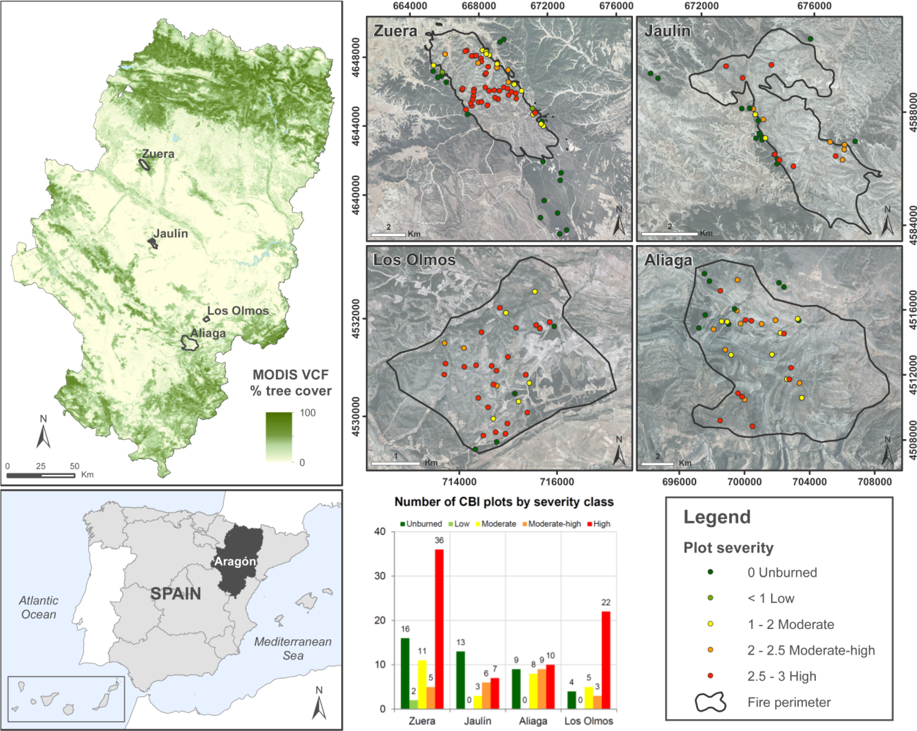
The Autonomous Region of Aragón, located in northeastern Spain (Figure 1), stretches from the Pyrenees range, in the north, to the Iberian range, in the south. Aragón is the northernmost semi-arid region in Europe, although it is crossed by the Ebro River Valley at its center. The geological diversity of this area results in high topographic variation: The Pyrenees rise to more than 3000 m.a.s.l. and extend their foothills, the pre-Pyrenees, southward to the Ebro basin, gradually decreasing in elevation up to 100 m.a.s.l.
In the central sector of the Ebro Valley, annual precipitation is low, averaging 350 mm and mostly occurring in autumn and spring. Its Mediterranean continental climate [41] presents cold winters, with monthly mean temperature about 7 °C, and hot, dry summers, with mean temperatures about 24 °C. However, altitude and topographic barriers modify this general pattern of extreme aridity at the edge of the Ebro Basin by increasing humidity and diminishing temperatures, while keeping the same pattern of seasonal rain and drought as the center of the Ebro valley.
Approximately, 50% of the 1.5 million hectares of forested areas in Aragón are composed of coniferous forest, 35% correspond to mixed forest, and the rest is covered by deciduous forest. Open forests, with less than 20% of tree cover, and shrublands occupy another one million hectares. Over the last few decades, the area covered by forest increased as a result of afforestation projects and agricultural abandonment. The main tree species are Pinus halepensis P. Mill., Pinus sylvestris L., Pinus pinaster Soland., non Ait., Quercus ilex L., and Quercus pyrenaica Willd. The species Quercus coccifera L., Juniperus oxycedrus L. subsp. macrocarpa (Sibth. & Sm.) Ball, and Thymnus vulgaris L. are commonly encountered in shrublands [20].
Wildfires have significantly increased in the last twenty years, both in number and total area. The increase was related not only to weather conditions, but also to human activity. In Aragón, approximately 5000 ha are affected annually by fire. Almost 3000 ha of this burned land are forested areas. In exceptional years such as 1994 and 2009, the affected area reached up to 30000 ha. In 2008 and 2009, eight large fires (>100 ha) were declared in Aragón and the total affected area was around 23,000 ha, most of which was burned in 2009. All of the fires affected pine forests after a period of extremely dry and hot weather. In six of those fires the cause of ignition was lightning while the remaining two were ignited due to anthropogenic activities [20]. Four of these fires (Figure 1) were analyzed in this study as a consequence of their significant environmental impact due to their large extension (Table 1).
2.2. Field Data Collection
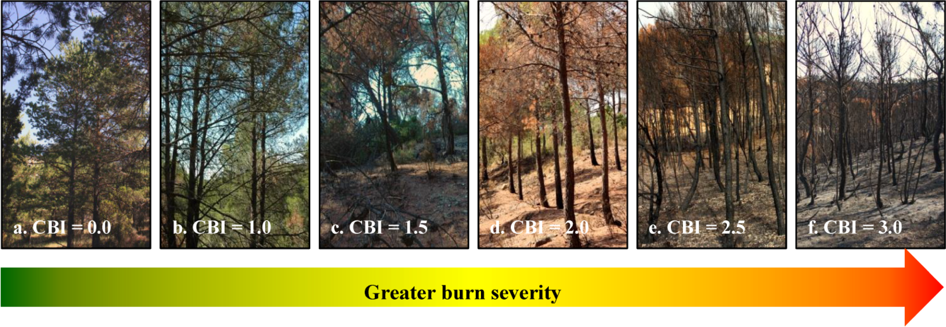
Field data were collected within two months after each fire utilizing the Composite Burn Index (CBI) field protocol, which takes into account the visible and averaged burn severity condition found in a plot [11]. Circular plots of 30 m diameter were laid out in areas of homogeneous fire effects using a Trimble GeoExplorer GPS with a positioning error at the center of the plot lower than 1 m after differential correction. Digital photos were taken from the center of each plot to the four cardinal directions to provide qualitative information about vegetation structure and soil conditions. The CBI assessment is a somewhat subjective estimation of the entire averaged burn severity across five forest strata: substrates, herbaceous vegetation, large shrubs and small trees, intermediate trees, and dominant and co-dominant canopy trees. The CBI for the whole plot area is based on synoptic scores ranging from 0 (not-burned) to 3 (completely burned) as described by Key and Benson [11]. To reduce any assessor bias, CBI assessments were conducted by the same two individuals.
Concerning fire effects in Aragón, low severity areas were characterized by scorched trees blackened at the base, charred to partially consumed litter while the understory layer was affected in a patchy pattern. The foliage and smaller twigs of the understory were partially to completely consumed, while branches were mostly intact. The tree crowns remained largely unaffected. In moderate severity areas, part of the understory layer was preserved. The needles or leaves and the small stems of the short shrubs (<1 m height) were consumed, whereas the tall shrubs (>1 m height) presented scorched foliage. The tree crowns were partially scorched, which resulted in incomplete foliage loss. For moderate–high severity areas, the consumption of the understory layer increased, whereas the tree crowns were usually scorched, with the foliage being retained only partially. The loss of branches and twigs was small for the overstory. The understory layer lost the twigs and small branches, especially the small shrubs (i.e., less than 1 m tall). In high severity areas, the combustion of the litter, understory layer, and tree crown elements (i.e., needles and twigs) was complete. At the highest severities, small- and medium-sized branches were also consumed. For more detail on the field sampling, see Tanase et al. [20].
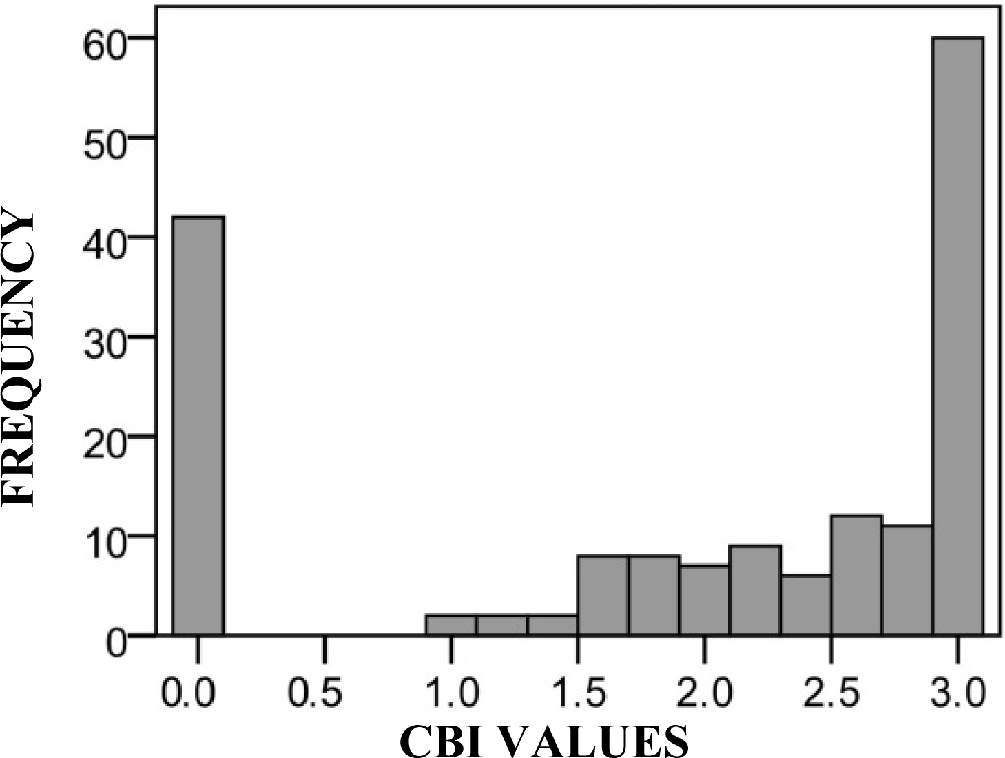
A selection of 169 from the initial 247 plots collected by Tanase et al. [20] was used in order to avoid areas where post-fire forest management activities, impacting canopy structure, had been carried out. For this reason, the 169 sampled plots do not represent proportionally the entire severity range (Figure 2). Table 2 shows the number of plots located in each severity range and how most of the plots were located in unburned or high severity areas.
2.3. ALS Acquisition
The ALS data were provided by the Spanish National Plan for Aerial Orthophotography (PNOA) [42] and captured, in several surveys conducted between 1 August 2010 and 5 February 2011, using two distinctive airborne sensors, Leica ALS60 and ALS50-II laser scanners. Data were delivered in LAS binary file format containing X and Y coordinates (UTM Zone 30 ETRS 1989), ellipsoidal elevation Z (ETRS 1989), with up to four returns measured per pulse, and intensity values from a 1064 nm wavelength laser. The resulting ALS nominal point density was 0.5 points/m2 with a vertical accuracy of less than 0.20 m. It should be noted that no difference exist between the ALS datasets in terms of sensing characteristics (i.e., operating principles) because PNOA mission ensures homogeneous flight campaigns and products. Moreover, the seasonality did not affect the coherence of the acquisitions because the study site is covered entirely by evergreen vegetation.
ALS Processing
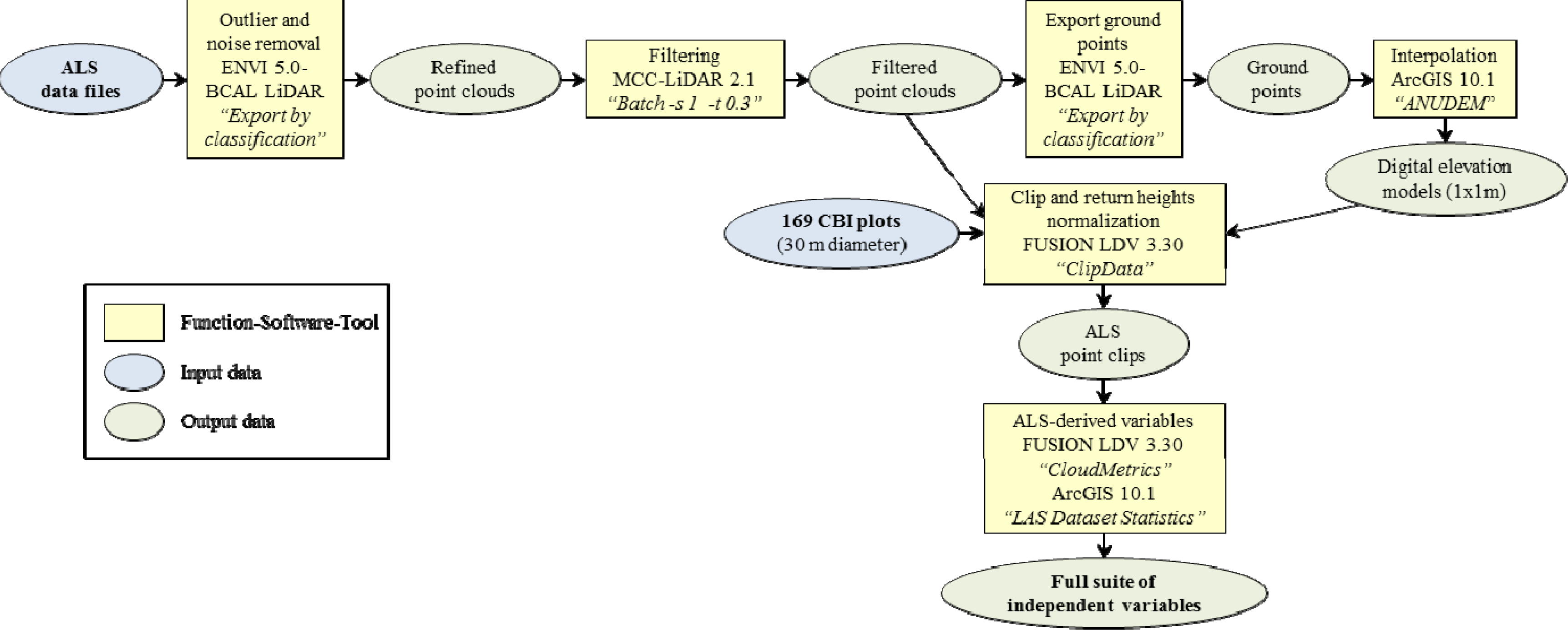
The ALS data set was provided in fifty-six 2 × 2 km tiles of raw data points which needed pre-processing before being filtered. Outliers and noise were removed with the open-source BCAL LiDAR module, developed by Idaho State University, Boise Center Aerospace Laboratory (BCAL), implemented in ENVI 5.0 (Boulder, CO, USA). Afterwards, the point cloud was filtered using MCC-LIDAR 2.1 command-line tool for processing discrete-return ALS data in forested environments [43]. The process classifies data points iteratively as ground or non-ground using the Multiscale Curvature Classification (MCC) algorithm developed by Evans and Hudak [44]. According to Montealegre et al. [45], this classification algorithm, based on identifying non-ground points that exceed positive curvature thresholds across multiple scales, balances commission and omission errors in forestry applications. Subsequently, a high-resolution (1 m) bare earth digital elevation model (DEM), was created from the ground points using ANUDEM interpolation implemented in ArcGIS 10.1 software (ESRI, Redlands, CA, USA). ANUDEM uses a thin plate spline method where a smooth surface is constructed from the irregularly spaced ALS points [46]. Finally, the ALS point elevations were normalized by subtracting off the elevation of the underlying terrain, represented by the DEMs previously created, to obtain estimates of aboveground height for each return. This subtraction was performed using FUSION LDV 3.30 open source software [47], developed by the Remote Sensing Applications Center (USDA).
With the aim of getting statistical information about the laser returns in order to estimate fire severity, a full suite of independent variables (Table 3) commonly used in vegetation modelling [48] was generated with “ClipData” and “CloudMetrics” commands included in FUSION LDV 3.30 [49] and with “LAS Dataset” tool in ArcGIS 10.1. The computation was performed at plot level (30 m diameter). A flowchart of the ALS data processing is presented in Figure 3.
2.4. Data Analysis
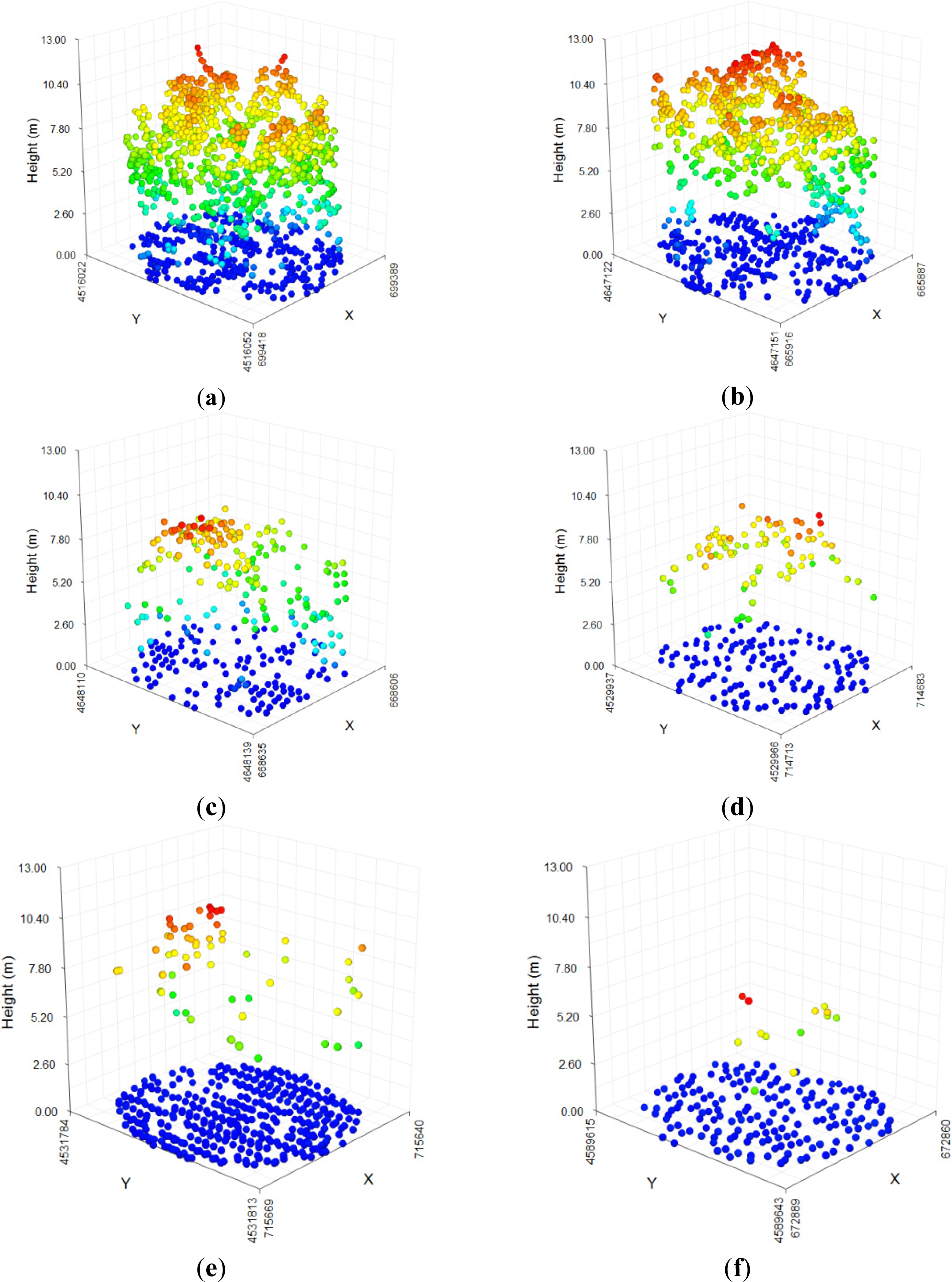
The steps followed in the methodology used to evaluate the relationship between the dependent (CBI) and independent (ALS-derived) variables are presented in Table 4. The Spearman’s rank correlation coefficient was used with the purpose of assessing the statistical dependence between plot severity and each ALS variable. A linear regression analysis was rejected as the assumption of normality of the CBI dataset was not met, even after transforming the variables. Thus, a logistic regression analysis, which requires splitting the CBI values into null or low severity and high severity, was selected. Therefore, the Kruskal–Wallis test was used for testing whether the mean values and distribution of the independent variables in both groups (null or low severity and high severity) are statistically different. This test is commonly used to select the most significant variables to be introduced in logistic regression analysis when it is not possible to assume normality and homoscedasticity of the samples [50]. As mentioned above, the dataset was split into two categories, null-low burn severity (CBI value ≤ 1.5) and high burn severity (CBI value > 1.5) to carry out this non-parametric method. The selection of the threshold value 1.5 was based on a qualitative analysis of the ALS point clouds and corresponding values of severity. The CBI method is based on a visual analysis of the magnitude of the environmental change with respect to the presumed pre-fire state. Therefore, given the information collected in the CBI forms such as the percentage of canopy mortality in big and intermediate trees, the depth of burn, percentage of the foliage altered, and the degree of change in vegetation strata, it was analyzed visually how these changes are reflected in the point clouds at plot level. Wildfire disturbance influences the horizontal and vertical structure of vegetation [34,51], which is recorded by ALS returns (Figure 4). However, as we only had post-fire information and it was not possible to estimate the structural change, it was assumed that the pre-fire structure of vegetation was homogeneous and similar to areas not affected by fire inside or near the fire perimeter (Figure 5a). Figure 5 depicts some examples of normalized point clouds in plots with different CBI values. The loss of canopy and the forest opening where logs remain without foliage are the most relevant indicators captured by the ALS. As can be observed in Figure 5, point clouds are relatively dense and homogeneous for CBI values up to 1.5 and from that value onwards, the amount of returns decrease more significantly because the tree crowns were partially scorched with incomplete foliage loss. Therefore, we assumed that ALS was able to distinguish plots with CBI values under 1.5 (null and low severity) and above 1.5 (high severity). CBI values above 1.5 present a general trend of loss of vegetation structure in the field, which manifests itself in the ALS point clouds.
As mentioned above, logistic regression analysis, one of the most frequently used multivariate statistical analysis, was selected due to the non-normal distribution of the variables [52,53]. It enables the creation of reliable predictive models from explanatory variables (either continuous or discrete). This technique, already used successfully to evaluate several phenomena—e.g., landslide hazard, water erosion, sinkhole susceptibility, human-caused ignition, etc.—evaluates the probability of an event occurrence (P) by estimating the possibility that a case will be classified into one of two mutually exclusive categories as opposed to the other category of the dependent dichotomous variable [54]. In this research, we used logistic regression to establish a functional relationship between the presence or not of fire impact within a plot in a binary-coded manner (1 = high burn severity; 0 = absence or low burn severity) and the set of the independent variables derived from ALS data. This can be written as:
As the acceptance of a model requires the evaluation of its robustness to small changes of the input data, CBI data were split into two different samples. A random selection of 118 cases (70% of the sample) was used as a training subset, while the 51 unselected cases were used to test the accuracy of the model. Well-balanced samples were considered in terms of proportion of plots with high and low fire severity values. A forward stepwise (likelihood ratio) method was applied [55] to the training dataset in order to select the explanatory variables and to obtain several models. These models were evaluated by computing the Cox and Snell and the Nagelkerke pseudo-R2 tests, the log likelihood (-2LL) statistic and the chi-square test in order to calculate how strong the relationship between the explanatory variables and the outcome was. The Hosmer and Lemeshow test is similar to a chi-square test, and it indicates the extent to which the model provides better fit than a null model with no predictors, i.e., how well the model fits the data, as in log-linear modelling. The significance was assessed individually for each independent variable incorporated in the model by means of the Wald test [50,54].
The model was selected based on the principle of parsimony that implies a preference of models with a smaller number of parameters as each parameter introduced into the model adds some uncertainty to it, considering the significance level of individual predictor variables, as well as the usefulness of the model.
Logistic models are frequently used in a classification approach by selecting a given value of the response variable (the probability of high fire severity, in our case) and classifying all resulting values in one of two groups (1 or 0) according to it. The threshold value is normally the 0.5 probability, as usually the two sample groups are similar in size. However, for the case where the two groups are very dissimilar in size, the proportion of ones in the sample should be used instead of the 0.5 value [56,57]. Thus, value 1 was assigned to the predicted response when probability was greater than the cutoff value 0.6, specified by the proportion of CBI plots classified as 1 (CBI value > 1.5) in the observed values of the dependent variable.
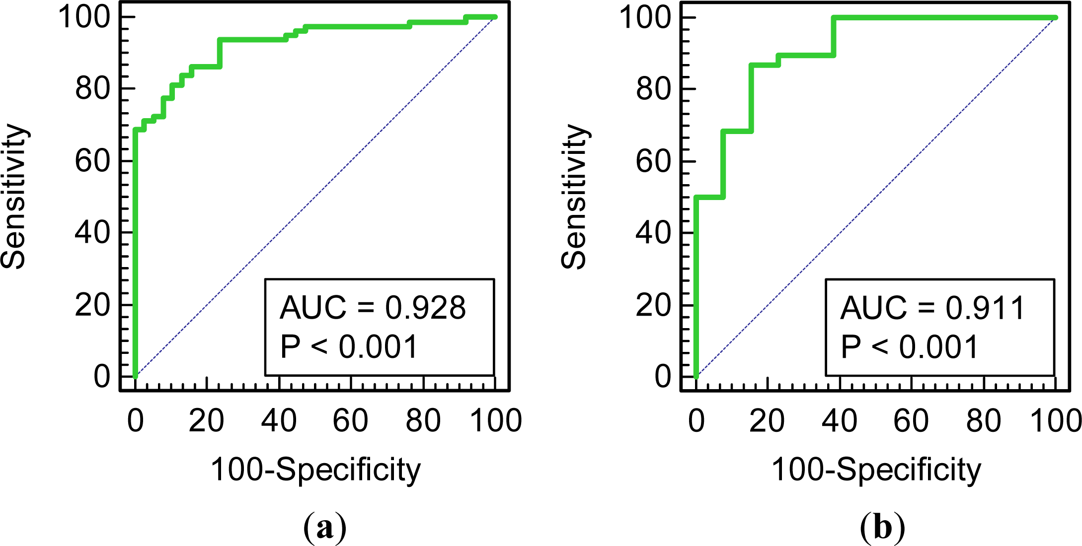
The accuracy of selected logistic regression model was tested by cross tabulation associated with Cohen’s Kappa index and the receiver operating characteristic (ROC) curves. The first is a statistical coefficient of inter-rater agreement that allows knowing if agreement is attributable to chance alone. Kappa index ranges generally from 0 to 1 (although negative numbers are possible). According to Landis and Koch [58], values of Kappa below 0.40 present poor agreement, from 0.40 to 0.75 are considered of good agreement, and above 0.75 generally reflect excellent agreement. In the case of ROC curves, the computed values of the area under the ROC curve (AUC) [59], provide a measure of goodness-of-fit of the logistic regression model based on the simultaneous measure of sensitivity (true positive) and specificity (true negative) for all possible cutoff points. Sensitivity is calculated as the fraction of CBI plots that were correctly classified as high burn severity, while specificity is derived from the proportion of CBI plots that were properly categorized as low burn severity. The closeness of the ROC curve to the upper left corner (AUC = 1) indicates a high accuracy of the model (i.e., a correct discrimination between positive and negative cases). In relation to the computed AUC value, Hosmer and Lemeshow [52] classify a predictive performance as acceptable (AUC > 0.7), excellent (AUC > 0.8) or outstanding (AUC > 0.9).
Finally, the intercept and the weights of the variables included in the selected regression model were implemented in ArcGIS 10.1 using map algebra to generate categorical maps of fire severity. The spatial resolution of the maps was 25 m cell size, which was determined by the area of the sampled CBI plots. In seeking a useful map to assist land management purposes rather than a dichotomous response (presence or absence of fire impact), one of the methods adopted in literature is to divide the histogram of the probability map into different categories based on expert opinions [60]. This type of changing continuous data into two or more categories does not take into account the relative position of a case within the probability map and is neither fully automated nor statistically tested. Thus, in this study, we also considered alternative classification systems that use natural breaks, equal intervals and standard deviations. In addition, we also tested a manual classification of the probability values based on a direct relationship with the categories established by the CBI protocol: Unburned (CBI = 0), Low (CBI ≤ 1), Moderate (1 < CBI ≤ 2), Moderate–High (2 < CBI ≤ 2.5) and High (CBI > 2.5). The selection of the final classification approach was based on its suitability to the information and the scale of investigation.
Finally, it should be noted that due to the lack of pre-fire information our model is only valid in areas that were covered by homogeneous pine stands before fire occurrence, so the final map only represent estimates of severity for those areas.
3. Results
3.1. Correlation Analysis and Logistic Regression Model
Among the 51 explanatory variables derived from ALS data, 32 had a moderate–high significant Spearman’s coefficient. Their correlation coefficients (rho) are reported in Table 5. Height variables, such as kurtosis (0.788) or the 25th percentile (−0.767) had the strongest correlation with burn severity. In addition, the percentage of all returns above 1 m (−0.757) or the percentage of first returns above 1 m (−0.744) also presented high correlation coefficients. In the case of height metrics with negative coefficients, higher values of the variable indicate a higher amount of pulses returned by the canopy structure implying lower severity values. For example, a higher 25th percentile (e.g., 2 m) indicates that 75% of returns present height values above 2 m (lower severity) while a lower 25th percentile (e.g., 0.19 m) indicates that 75% of returns present height values above 0.19 m (higher severity). This was also the case for variables related to percentage of returns above a height threshold: a high percentage of returns from the total number of returns above 1 m implies low severity values while lower percentage of returns represent higher severity values. In contrast, variables as kurtosis and skewness presented positive coefficients indicating high number of returns from low heights (high severity) while negative coefficients corresponded to areas with a higher number of returns from higher heights (low severity).
Concerning the differences between the two groups (null or low severity and high severity), the 20th percentile (68.566) and the percentage of all returns above mean (67.337) presented the highest Kruskal-Wallis chi-square values, followed by the 25th percentile and the percentage of all returns above mean divided by all first returns (64.776 in both cases). In general, low height percentiles (between 40th and 20th), height distribution measures such as skewness, and the percentage of returns above a certain threshold showed statistically significant differences between high and low severity values (Table 6). According to these results, differences between severities are identified by ALS variables that are commonly assumed to be related to vegetation structure.
The logistic regression models created with the training dataset using a forward stepwise method to select the explanatory variables are summarized in Table 7. The -2LL and the likelihood ratio (LR) test with chi-square (X2) distribution evaluate the fitting of the logistic regression model to the observed data. Smaller -2LL values and higher X2 values indicate a better fitting with a statistical significance (p ≤ 0.05) [52,54]. Similar to linear regression, the pseudo-R2 values show approximately how much variation is explained by the model.
The final model selected was the second (step 2) due to the principle of parsimony, and because the rest of the models included no significant variables. Nagelkerke’s R2 suggests that this model explains roughly 66% of the variation and is composed by the percentage of all returns above 1 m and the canopy relief ratio as significant ALS-derived variables. The Hosmer and Lemeshow’s goodness-of-fit test confirms, since chi-square is not significant, that model two is an adequate fit. Table 8 shows the statistical significance of the individual predictors that entered in the selected model. The β coefficients of both variables are significant and negative, thereby indicating that the decrease in canopy relief ratio values and in the percentage of all returns above 1 m is associated with the increase in fire severity. The canopy relief ratio is a quantitative descriptor of the relative shape of the canopy (Table 3) ranging between 0 and 1 and reflecting the degree to which canopy surfaces are in the upper (>0.5) or the lower (<0.5) portion of the height interval [61]: for high burn severity, the canopy relief ratio value tends to 0, whereas the value is close to 0.5 for low burn severity (see Figure 2). The percentage of all returns above 1 m is sensitive to the amount of biomass located above the understory layer. If the percentage is low it means that treetops have been scorched by fire, with only tree trunks and some branches remaining, which indicates high burn severities.
3.2. Model Validation
The discrimination ability of the logistic regression model was tested by a cross-tabulation between observed and predicted high (1) and low (0) severity cases. Table 9 shows the percentage of agreement between observed and predicted values for both training and validation samples. Value 1 was assigned to the predicted value when the obtained probability was greater than the cutoff value (i.e., 0.6) quantified as the proportion of CBI plots classified as 1. Similar accuracies are achieved for both training and validation datasets with almost 85% of the cases being correctly classified. Furthermore, Cohen’s Kappa index summarized in Table 10 demonstrates a good agreement for both training and validation datasets (0.681 and 0.565, respectively).
Figure 6 presents the ROC curves and AUC values for both, the training and validation subsets of CBI plots. ROC curves are fairly similar and, consequently, very small differences of AUC values are observed with an asymptotic significance less than 0.05. Since, both the classification matrix and AUC values indicated that the modelling procedure carried out at sample plot scales has not suffered from over-fitting and the model demonstrates robustness.
3.3. Fire Severity Mapping
The final result of the regression process is the implementation of the model in a GIS environment with the aim of obtaining a spatial distribution of the fire severity probability (continuous values between 0 and 1) following Equation (2):
The more these numbers are close to 1, the higher the likelihood of finding a zone impacted by high fire severity. As mentioned above, a threshold of 0.6 (proportion of 1 in the sample) can be used to distinguish between the two categories used to generate the model: areas where fire severity is null or low or areas with high fire severity. However, for management purposes, it is sometimes more useful to develop categorical maps. A few trials showed that natural breaks-based, equal intervals and standard deviation classification systems based on the probability histogram values resulted in misleading maps. Since Spearman’s coefficient between CBI values and P probability showed a high correlation (0.807, p-value ≤ 0.01) the well-established CBI categories where used to divide the probability map in unburned, low, moderate, moderate–high and high fire severity: the average p values for each of the CBI classes were computed and subsequently used as central value for each severity range. This helped ensuring a better match between the observed values and those predicted by the logistic model. Table 11 presents the established categories of CBI value and the probability values assigned to them.
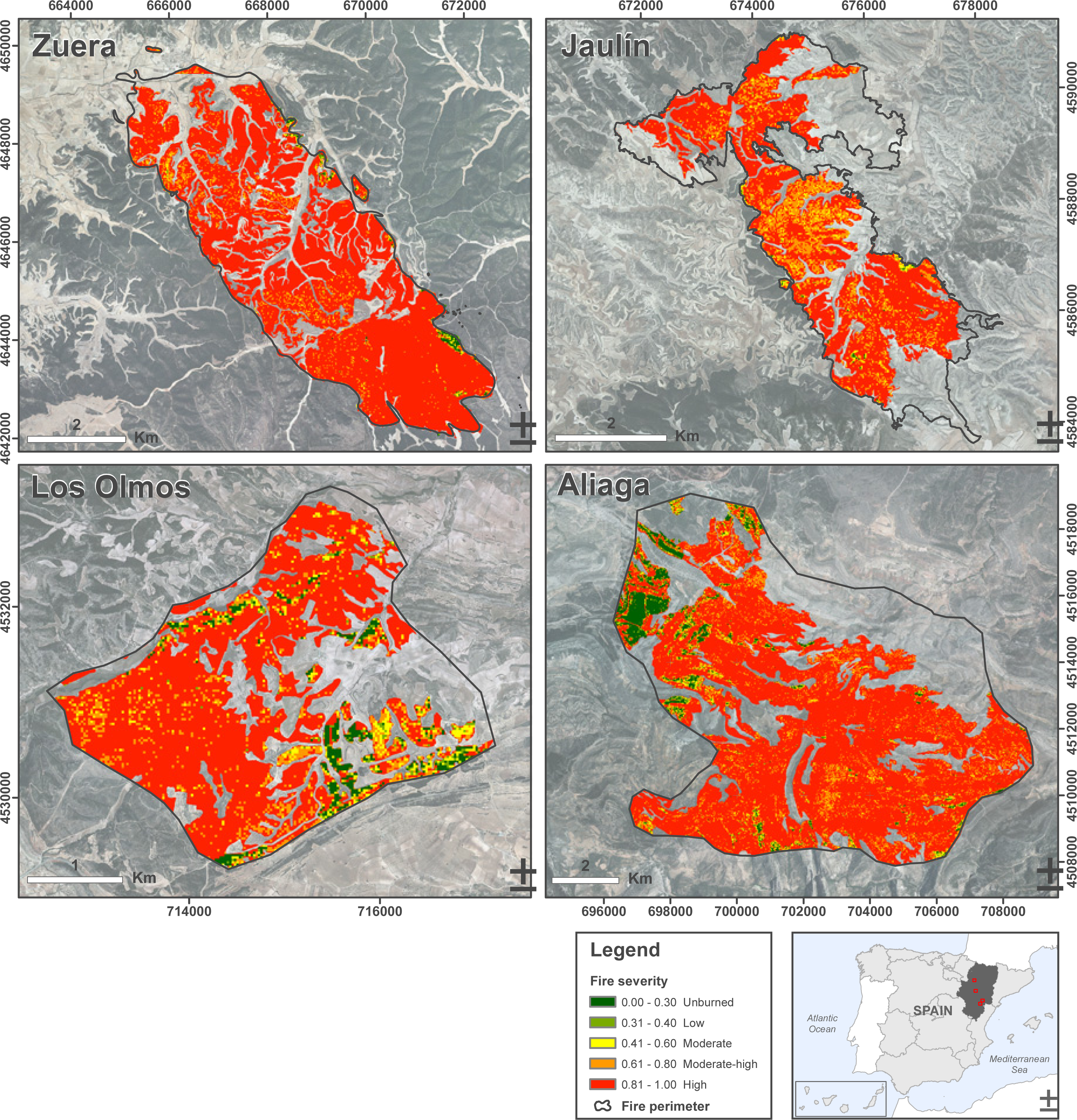
According to the above classification, Table 12 shows the percentage of fire severity within the fire perimeter by fire location. The results indicate that in Zuera the percentage of area affected by high fire severity was higher (91.16% of the total area inside of the fire perimeter). Conversely, Aliaga presented the highest percentage of area unaffected by fire, approximately 5.01%.
Figure 7 presents the probability map generated in a raster-GIS environment. Most of the area was affected by high or moderate–high burn severity, whereas low burn severity areas were mainly encountered along the fire borders. As mentioned above, our model fits well only in areas that were covered by homogeneous and continuous pine stands previous to fire occurrence and is only applicable to these areas. The lack of pre-fire information resulted in assigning high severity values to sparse canopy woodlands and crop lands which had to be masked out for the analysis.
4. Discussion
In the Mediterranean basin fire is a natural and historical element. However, in recent decades, fire recurrence and magnitude are profoundly altering forest ecosystems, with forest degradation being the most immediate effect. The main objective of this study was to evaluate the suitability of ALS-derived variables to estimate fire severity in four burned areas in Aragón, Spain. Our aim was to establish relationships between CBI data collected in the field and different variables derived from ALS point clouds. However, due to the absence of pre-fire ALS flights the two data sources provide information of different characteristics. On one hand, the CBI index estimates the change in the ecosystem after fire with respect to a previous situation using qualitative parameters that are then encoded into ranges of burn severity. On the other hand, the ALS data only provided estimations of vegetation structure after fire and not the vegetation change. Thus, we assumed homogeneous and continuous pre-fire vegetation in all field plots as reported by Tanase et al. [20]. Given these assumptions, a strong relationship was found between ALS-derived variables related to vegetation structural parameters and fire severity values, allowing the establishment of a model for fire severity mapping.
Kane et al. [34] noted the significant effects of fire on forest structure by using ALS data with Landsat-derived estimates of fire severity to measure the impact of fires over large areas. As fire severity increased, the canopy cover decreased while the number of tree clumps increased, indicating progressive canopy fragmentation. The work confirmed the utility of Landsat-based fire severity estimates and the utility of high resolution of ALS data to measure the structural change resulting from that process. This is one of the first approaches to fire severity assessment using ALS data; however, according to our knowledge, our work represents for the first time fire severity modelled using ALS-derived variables in relation to CBI field data, joining a small but growing body of literature focused on deriving fire severity estimates from ALS data [21,24,34,51].
The lack of pre-fire forest structure information derived from ALS data may be solved in the future by periodical acquisitions within the PNOA mission. Wang et al. [62] demonstrated high fire-severity accuracies (84%) in a rangeland ecosystem using pre- and post-fire ALS data. Their approach was based on evaluating changes in vegetation average height using pre- and post-fire ALS data, which was subsequently related to biomass combustion. However, the growing availability of ALS datasets with increasing nominal point density, combined with methods such as the one discussed in this paper, can assist forest management planning even when pre-fire ALS data are not available.
The way fire severity is distributed is a key factor in quantifying the impact of fires and post-fire management [9], as well as the ecosystem responses. The severity mapping attempts to identify problematic areas and help managers in allocating resources and restoration efforts and thus decreasing time and economic costs associated with field-work. Logistic regression was selected due to its ability to work with different types of independent variables, even when they are auto-correlated as well as due to its independency from data statistical distribution [55]. The method allowed for generating severity maps with up to 85.8% prediction accuracy when assessing spatial distribution of fire impact within pine forests. In addition, this research contributes to the creation of sensible theories about which explanatory variables are most important for fire severity estimation from low density ALS data, such as ALS measures of canopy shape and percentage of all returns above one meter.
Our research, like many ALS-based studies, lacked concurrent field and ALS acquisitions [24]. However, the evergreen character of species present in the study area compensated for such discrepancies. On the contrary, at the time of the ALS flight, some of the affected forests were felled and removed by forest management agencies. Field plots located in such areas were removed from analysis, considerably reducing the initial sampling to only 169 plots. In addition, the time gap could have diminished the accuracy of burn severity predictions due to the increasing vegetation recovery, especially in sprouting shrubs such as Quercus coccifera L.
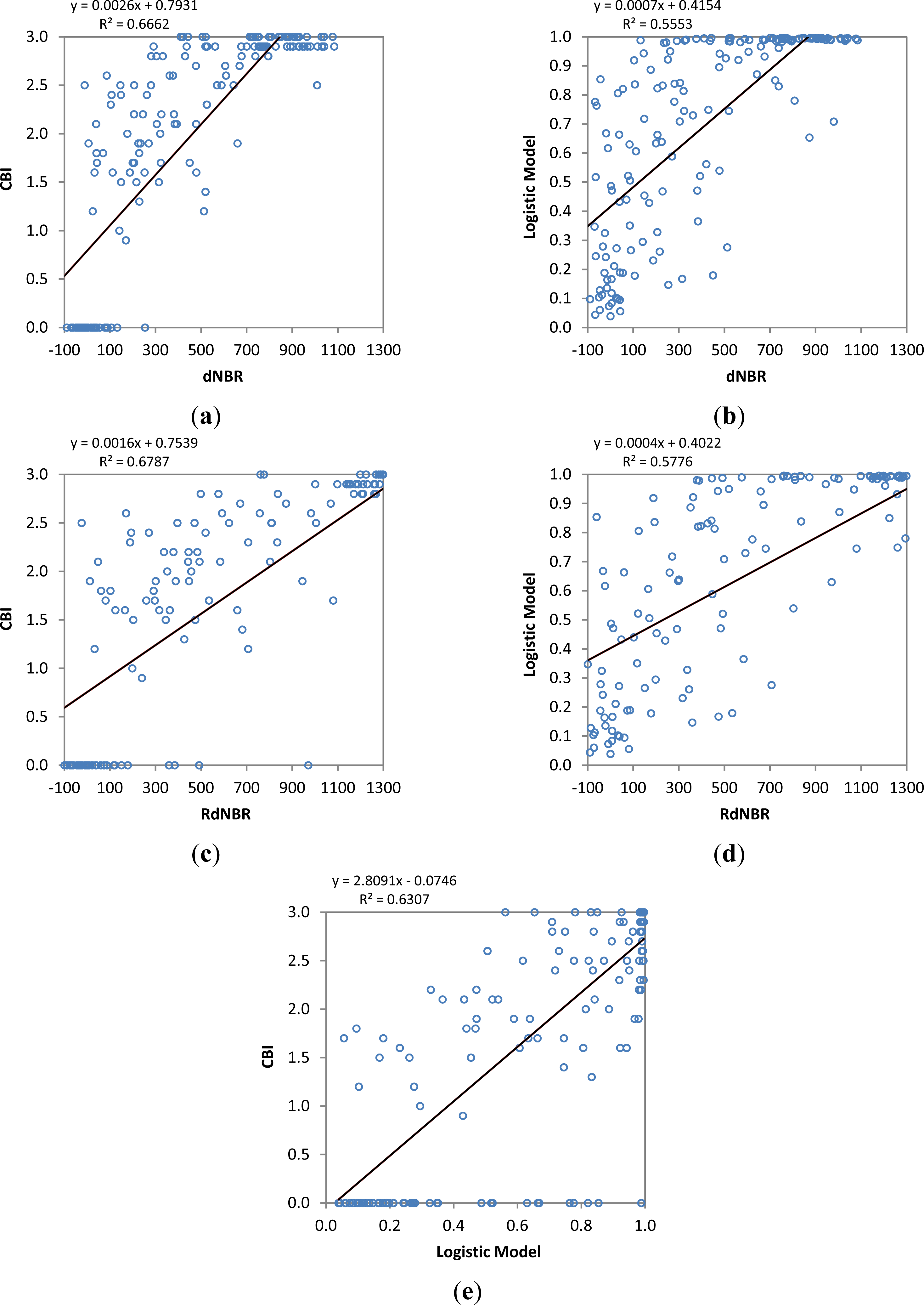
In order to determine whether ALS-derived fire severity estimations produce a better relationship than differenced Normalized Burn Ratio (dNBR) and its relative form (RdNBR) Landsat TM-based indices, the results of applying these indices, computed by Tanase et al. [20], and the results of our logistic model were correlated with CBI field plots data. The dNBR (Figure 8a) resulted in an R2 of 0.67, the RdNBR model (Figure 8c) achieved a R2 of 0.68 and the logistic model resulted in an R2 of 0.63. These coefficients of determination indicate that the relationship between observed data (CBI values) and the predicted severity from ALS logistic model is good but it does not exceed the coefficients obtained for the RdNBR and dNBR. Nevertheless, the ALS-based model, lacking pre-fire information, yields similar accuracy to optical approaches that used pre- and post-fire information. On the other hand, the relationship between our logistic model and Landsat-derived indices is moderate (Figure 8b,d), being better with RdNBR (R2 = 0.58) than with dNBR. Although all the approaches obtained good results, clearly there is still no perfect index for mapping fire effects. We therefore need to further investigate in this direction.
Accurately mapping the distribution of severity patches is important for site level recovery projects and for understanding overall landscape patterns created by fire. Thus, a detailed examination of the relation of established CBI classes and the values obtained with the logistic model, RdNBR and dNBR were performed. Then, we created and mapped five severity categories based on the mean values obtained at each CBI class.
Table 13 shows the category ranges obtained, the Kappa index of agreement between the CBI classes and the categories obtained with the three different approaches and the percentage of agreement in each category. As can be observed, the logistic regression approach led to under-representing low to moderate–high severity patches but presents better accuracy in the high severity class (89.33%accuracy) than RdNBR (86.67%) and dNBR (77.33%).
In our opinion, minimizing classification errors in high severity class is beneficial to land managers as it allows a better identification of areas that are severely burned [63]. However, to improve classification results, other methods such as random forests and nearest neighbor imputation could allow multiple severity classes mapping.
The integration of optical remotely sensed imagery, well suited for capturing horizontally distributed forest conditions, along with ALS variables that are more appropriate for capturing vertical forest structure, may improve fire severity assessment [64]. Finally, we are of the opinion that the generation of indices derived from pre- and post-fire ALS variables will considerably improve fire severity mapping.
5. Conclusions
This study presents a new methodological approach combining ALS-derived variables and field-assessed CBI, in order to estimate the impact of wildland fire across four sites in Aragón, northeastern Spain. Our work is unique in examining fire severity within this particular setting, i.e., Mediterranean pine forests and low-density ALS data (0.5 pulses/m2). We have demonstrated that ALS-derived variables from plot-level distributions of pulse return heights provide initial support for assessing the impact caused by fire. Height variables such as kurtosis or the 25th percentile of returns heights presented the highest correlation with CBI values (0.788 and, respectively, −0.767). The difference between high and low severity classes was best estimated using the 20th percentile and the percentage of all returns above mean which presented the highest Kruskal–Wallis chi-square values (68.566 and 67.337, respectively). Low percentiles (between 40th and 20th), skewness, and some percentages of ALS returns above a threshold, such as the average height, also showed significant differences between the two groups of severity.
The relationships between CBI data and a set of ALS point cloud variables have been assessed by means of forward stepwise logistic regression. The prediction power of the obtained model was tested using independent validation samples. The results show a fairly acceptable overall accuracy, confirming that logistic regression is an effective tool for fire severity analysis. Continuous fire severity maps were derived based on the probabilities obtained from the logistic model at plot level. Next, the average of those probabilities for each severity class allowed for the split of the map in fire severity classes. The lack of pre-fire forest structure information can be a handicap that could be solved by periodical acquisition of ALS datasets in the coming years.
Acknowledgments
This work has been financed by the Government of Aragón, Department of Science, Technology and University (FPI Grant BOA 30, 11/02/2011). The ALS data were provided by the National Center for Geographic Information of Spain. Francisco Palú, Marco Lorenzo and Emilio Pérez Aguilar from the Provincial Environment Service, Government of Aragón are also acknowledged for their help with the forest management activities carried out after the fires.
Author Contributions
Juan de la Riva had the original idea for the study. Antonio L. Montealegre and M.T. Lamelas developed the methodology and performed the analysis. Field data was provided by Mihai A. Tanase. Antonio L. Montealegre wrote the manuscript, incorporating suggestions from all authors, who approved the final manuscript.
Conflicts of Interest
The authors declare no conflict of interest.
References
- Bond, W.J.; Keeley, J.E. Fire as a global “herbivore”: The ecology and evolution of flammable ecosystems. Trends Ecol. Evol 2005, 20, 387–394. [Google Scholar]
- Amraoui, M.; Liberato, M.L.R.; Calado, T.J.; DaCamara, C.C.; Coelho, L.P.; Trigo, R.M.; Gouveia, C.M. Fire activity over Mediterranean Europe based on information from Meteosat-8. For. Ecol. Manag 2013, 294, 62–75. [Google Scholar]
- Ichoku, C.; Giglio, L.; Wooster, M.J.; Remer, L.A. Global characterization of biomass-burning patterns using satellite measurements of fire radiative energy. Remote Sens. Environ 2008, 112, 2950–2962. [Google Scholar]
- Oliveira, S.; Oehler, F.; San-Miguel-Ayanz, J.; Camia, A.; Pereira, J.M.C. Modeling spatial patterns of fire occurrence in Mediterranean Europe using multiple regression and random forest. For. Ecol. Manag 2012, 275, 117–129. [Google Scholar]
- Pausas, J.G.; Llovet, J.; Rodrigo, A.; Vallejo, R. Are wildfires a disaster in the Mediterranean basin?—A review. Int. J. Wildland Fire 2008, 17, 713–723. [Google Scholar]
- San-Miguel-Ayanz, J.; Moreno, J.M.; Camia, A. Analysis of large fires in European Mediterranean landscapes: Lessons learned and perspectives. For. Ecol. Manag 2013, 294, 11–22. [Google Scholar]
- Eleazar, M.J.; Enríquez, E.; Gallar, J.J.; Jemes, V.; López, M.; Mateo, M.L.; Muñoz, A.; Parra, P.J. Los Incendios Forestales en España, Decenio 2001–2010; Área de Defensa contra lncendios Forestales (ADCIF) del Ministerio de Agricultura, Alimentación y Medio Ambiente: Madrid, Spain, 2012; p. 138. [Google Scholar]
- Collins, R.D.; de Neufville, R.; Claro, J.; Oliveira, T.; Pacheco, A.P. Forest fire management to avoid unintended consequences: A case study of Portugal using system dynamics. J. Environ. Manag 2013, 130, 1–9. [Google Scholar]
- Chuvieco, E. Earth Observation of Wildland Fires in Mediterranean Ecosystems; Springer: Alcalá de Henares, Spain, 2009; p. 257. [Google Scholar]
- De Santis, A.; Chuvieco, E. Burn severity estimation from remotely sensed data: Performance of simulation vs. empirical models. Remote Sens. Environ 2007, 108, 422–435. [Google Scholar]
- Landscape Assessment (LA) Sampling and Analysis Methods. Available online: http://www.fs.fed.us/rm/pubs/rmrs_gtr164/rmrs_gtr164_13_land_assess.pdf (accessed on 5 May 2014).
- Epting, J.; Verbyla, D.; Sorbel, B. Evaluation of remotely sensed indices for assessing burn severity in interior Alaska using Landsat TM and ETM+. Remote Sens. Environ 2005, 96, 328–339. [Google Scholar]
- Kasischke, E.S.; Turetsky, M.R.; Ottmar, R.D.; French, N.H.F.; Hoy, E.E.; Kane, E.S. Evaluation of the composite burn index for assessing fire severity in Alaskan black spruce forests. Int. J. Wildland Fire 2008, 17, 515–526. [Google Scholar]
- De Santis, A.; Chuvieco, E. GeoCBI: A modified version of the composite burn index for the initial assessment of the short-term burn severity from remotely sensed data. Remote Sens. Environ 2009, 113, 554–562. [Google Scholar]
- Loboda, T.V.; French, N.H. F.; Hight-Harf, C.; Jenkins, L.; Miller, M.E. Mapping fire extent and burn severity in Alaskan tussock tundra: An analysis of the spectral response of tundra vegetation to wildland fire. Remote Sens. Environ 2013, 134, 194–209. [Google Scholar]
- Hall, R.J.; Freeburn, J.T.; de Groot, W.J.; Pritchard, J.M.; Lynham, T.J.; Landry, R. Remote sensing of burn severity: experience from western Canada boreal fires. Int. J. Wildland Fire 2008, 17, 476–489. [Google Scholar]
- Veraverbeke, S.; Verstraeten, W.W.; Lhermitte, S.; Goossens, R. Evaluating landsat thematic mapper spectral indices for estimating burn severity of the 2007 Peloponnese wildfires in Greece. Int. J. Wildland Fire 2010, 19, 558–569. [Google Scholar]
- Hudak, A.T.; Morgan, P.; Bobbitt, M.J.; Smith, A.M.S.; Lewis, S.A.; Lentile, L.B.; Robichaud, P.R.; Clark, J.T.; McKinley, R.A. The relationship of multispectral satellite imagery to immediate fire effects. Fire Ecol 2007, 3, 64–90. [Google Scholar]
- Van Wagtendonk, J.W.; Root, R.R.; Key, C.H. Comparison of AVIRIS and Landsat ETM+ detection capabilities for burn severity. Remote Sens. Environ 2004, 92, 397–408. [Google Scholar]
- Tanase, M.; de la Riva, J.; Pérez-Cabello, F. Estimating burn severity at the regional level using optically based indices. Can. J. For. Res 2011, 41, 863–872. [Google Scholar]
- Bergen, K.M.; Goetz, S.J.; Dubayah, R.O.; Henebry, G.M.; Hunsaker, C.T.; Imhoff, M.L.; Nelson, R.F.; Parker, G.G.; Radeloff, V.C. Remote sensing of vegetation 3-D structure for biodiversity and habitat: Review and implications for lidar and radar spaceborne missions. J. Geophys. Res 2009, 114, G00E06. [Google Scholar] [CrossRef]
- Tanase, M.A.; Santoro, M.; Wegmüller, U.; de la Riva, J.; Pérez-Cabello, F. Properties of X-, C- and L-band repeat-pass interferometric SAR coherence in Mediterranean pine forests affected by fires. Remote Sens. Environ 2010, 114, 2182–2194. [Google Scholar]
- Tanase, M.; de la Riva, J.; Santoro, M.; Pérez-Cabello, F.; Kasischke, E. Sensitivity of SAR data to post-fire forest regrowth in Mediterranean and boreal forests. Remote Sens. Environ 2011, 115, 2075–2085. [Google Scholar]
- Kane, V.R.; Lutz, J.A.; Roberts, S.L.; Smith, D.F.; McGaughey, R.J.; Povak, N.A.; Brooks, M.L. Landscape-scale effects of fire severity on mixed-conifer and red fir forest structure in Yosemite National Park. For. Ecol. Manag 2013, 287, 17–31. [Google Scholar]
- Vosselmann, G.; Maas, H.G. Airborne and Terrestrial Laser Scanning; Whittles Publishing: Dunbeath, UK, 2010. [Google Scholar]
- Lefsky, M.A.; Cohen, W.B.; Acker, S.A.; Parker, G.G.; Spies, T.A.; Harding, D. Lidar remote sensing of the canopy structure and biophysical properties of douglas-fir western hemlock forests. Remote Sens. Environ 1999, 70, 339–361. [Google Scholar]
- Naesset, E; Økland, T. Estimating tree height and tree crown properties using airborne scanning laser in a boreal nature reserve. Remote Sens. Environ 2002, 79, 105–115. [Google Scholar]
- Andersen, H.E.; McGaughey, R.J.; Reutebuch, S.E. Estimating forest canopy fuel parameters using LIDAR data. Remote Sens. Environ 2005, 94, 441–449. [Google Scholar]
- Zolkos, S.G.; Goetz, S.J.; Dubayah, R. A meta-analysis of terrestrial aboveground biomass estimation using lidar remote sensing. Remote Sens. Environ 2013, 128, 289–298. [Google Scholar]
- Kane, V.R.; Gersonde, R.F.; Lutz, J.A.; McGaughey, R.J.; Bakker, J.D.; Franklin, J.F. Patch dynamics and the development of structural and spatial heterogeneity in Pacific Northwest forests. Can. J. For. Res 2011, 41, 2276–2291. [Google Scholar]
- Reutebuch, S.E.; Andersen, H.-E.; McGaughey, R.J. Light detection and ranging (LIDAR): An emerging tool for multiple resource inventory. J. For 2005, 103, 286–292. [Google Scholar]
- Hudak, A.T.; Evans, J.S.; Smith, A.M.S. LiDAR utility for natural resource managers. Remote Sens 2009, 1, 934–951. [Google Scholar]
- Asner, G.P.; Hughes, R.F.; Mascaro, J.; Uowolo, A.L.; Knapp, D.E.; Jacobson, J.; Kennedy-Bowdoin, T.; Clark, J.K. High-resolution carbon mapping on the million-hectare Island of Hawaii. Front. Ecol. Environ 2011, 9, 434–439. [Google Scholar]
- Kane, V.R.; North, M.P.; Lutz, J.A.; Churchill, D.J.; Roberts, S.L.; Smith, D.F.; McGaughey, R.J.; Kane, J.T.; Brooks, M.L. Assessing fire effects on forest spatial structure using a fusion of Landsat and airborne LiDAR data in Yosemite National Park. Remote Sens. Environ 2013, 2013. org/10.1016/j.rse.2013.07.041. [Google Scholar]
- Agca, M.; Popescu, S.C.; Harper, C.W. Deriving forest canopy fuel parameters for loblolly pine forests in eastern Texas. Can. J. For. Res 2011, 41, 1618–1625. [Google Scholar]
- Erdody, T.L.; Moskal, L.M. Fusion of LiDAR and imagery for estimating forest canopy fuels. Remote Sens. Environ 2010, 114, 725–737. [Google Scholar]
- Riaño, D.; Chuvieco, E.; Condés, S.; González-Matesanz, J.; Ustin, S.L. Generation of crown bulk density for Pinus sylvestris L. from lidar. Remote Sens. Environ 2004, 92, 345–352. [Google Scholar]
- Riaño, D.; Chuvieco, E.; Ustin, S.L.; Salas, J.; Rodríguez-Pérez, J.R.; Ribeiro, L.M.; Viegas, D.X.; Moreno, J.M.; Fernández, H. Estimation of shrub height for fuel-type mapping combining airborne LiDAR and simultaneous color infrared ortho imaging. Int. J. Wildland Fire 2007, 16, 341–348. [Google Scholar]
- Mutlu, M.; Popescu, S.C.; Zhao, K. Sensitivity analysis of fire behavior modeling with LiDAR-derived surface fuel maps. For. Ecol. Manag 2008, 256, 289–294. [Google Scholar]
- Skowronski, N.S.; Clark, K.L.; Duveneck, M.; Hom, J. Three-dimensional canopy fuel loading predicted using upward and downward sensing LiDAR systems. Remote Sens. Environ 2011, 115, 703–714. [Google Scholar]
- Vicente-Serrano, S.M.; Lasanta, T.; Gracia, C. Aridification determines changes in forest growth in Pinus halepensis forests under semiarid Mediterranean climate conditions. Agric. For. Meteorol 2010, 150, 614–628. [Google Scholar]
- Spanish National Plan for Aerial Orthophotography (PNOA). Available online: http://www.ign.es/PNOA/vuelo_lidar.html (accessed on 30 December 2013).
- MCC-LiDAR Multiscale Curvature Classification for LiDAR data. Available online: http://sourceforge.net/p/mcclidar/wiki/Home/ (accessed on 2 April 2014).
- Evans, J.S.; Hudak, A.T. A Multiscale curvature algorithm for classifying discrete return LiDAR in forested environments. IEEE Trans. Geosci. Remote Sens 2007, 45, 1029–1038. [Google Scholar]
- Montealegre, A.; Lamelas, T.; de la Riva, J. Evaluación de Métodos de Filtrado Para la Clasificación de la Nube de Puntos del Vuelo LiDAR PNOA. In Teledetección. Sistemas Operacionales de Observación de la Tierra; Fernández-Renau González-Anleo, A., de Miguel Llanes, E., Eds.; INTA: Madrid, Spain, 2013; pp. 184–187. [Google Scholar]
- Hutchinson, M.F.; Xu, T.; Stein, J.A. Recent Progress in the ANUDEM Elevation Gridding Procedure. Proceedings of the Geomorphometry, 2011, Redlands, CA, USA, 7–9 September 2011; pp. 19–22.
- Fusing LIDAR Data Photographs Other Data Using 2D and 3D Visualization Techniques. Avaliable online: http://www.fs.fed.us/pnw/olympia/silv/publications/opt/488_McGaugheyCarson (accessed on 29 April 2014).
- Evans, J.; Hudak, A.; Faux, R.; Smith, A.M. Discrete return Lidar in natural resources: Recommendations for project planning, data processing, and deliverables. Remote Sens 2009, 1, 776–794. [Google Scholar]
- González-Olabarria, J.-R.; Rodríguez, F.; Fernández-Landa, A.; Mola-Yudego, B. Mapping fire risk in the model forest of urbión (Spain) based on airborne LiDAR measurements. For. Ecol. Manag 2012, 282, 149–156. [Google Scholar]
- Álvarez Cáceres, R. Estadística Multivariante y No Paramétrica con SPSS: Aplicación a las Ciencias de la Salud; Díaz de Santos: Madrid, Spain, 1994; p. 408. [Google Scholar]
- Angelo, J.J.; Duncan, B.W.; Weishampel, J.F. Using lidar-derived vegetation profiles to predict time since fire in an oak scrub landscape in East-Central Florida. Remote Sens 2010, 2, 514–525. [Google Scholar]
- Hosmer, D.W.; Lemeshow, S. Applied Logistic Regression; Wiley: Hoboken, USA, 2000. [Google Scholar]
- Hair, J.F.; Anderson, R.E.; Tatham, R.L.; Black, W.C. Análisis Multivariante, 5th ed; Prentice Hall Iberia: Madrid, Spain, 1999. [Google Scholar]
- Conoscenti, C.; Angileri, S.; Cappadonia, C.; Rotigliano, E.; Agnesi, V.; Märker, M. Gully erosion susceptibility assessment by means of GIS-based logistic regression: A case of Sicily (Italy). Geomorphology 2014, 204, 399–411. [Google Scholar]
- Menard, S. Logistic Regression: From Introductory to Advanced Concepts and Applications; SAGE: Thousand Oaks, CA, USA, 2010; p. 392. [Google Scholar]
- Lamelas, M.T.; Marinoni, O.; Hoppe, A.; de la Riva, J. Dollines probability map using logistic regression and GIS technology in the central Ebro Basin (Spain). Environ. Geol 2008, 54, 963–977. [Google Scholar]
- Beguería, S.; Lorente, A. Landslide Hazard Mapping by Multivariate Statistics: Comparison of Methods and Case Study in the Pyrenees, Instituto Pirenaico de Ecología, Contract No. EVG1-CT-1999–00007. Available online: http://damocles.irpi.pg.cnr.it/docs/reports/df_modelling.pdf (accessed on 29 April 2014).
- Landis, J.R.; Koch, G.G. The measurement of observer agreement for categorical data. Biometrics 1977, 33, 159–174. [Google Scholar]
- Hanley, J.A.; McNeil, B. The meaning and use of the área under a receiver operating characteristic (ROC) curve. Radiology 1982, 143, 29–36. [Google Scholar]
- Ayalew, L.; Yamagishi, H. The application of GIS-based logistic regression for landslide susceptibility mapping in the Kakuda-Yahiko Mountains, Central Japan. Geomorphology 2005, 65, 15–31. [Google Scholar]
- Parker, G.G.; Russ, M.E. The canopy surface and stand development: Assessing forest canopy structure and complexity with near-surface altimetry. For. Ecol. Manag 2004, 189, 307–315. [Google Scholar]
- Wang, C.; Glenn, N.F. Estimation of fire severity using pre- and post-fire LiDAR data in sagebrush steppe rangelands. Int. J. Wildland Fire 2009, 18, 848–856. [Google Scholar]
- Miller, J.D.; Thode, A.E. Quantifying burn severity in a heterogeneous landscape with a relative version of the delta Normalized Burn Ratio (dNBR). Remote Sens. Environ 2007, 109, 66–80. [Google Scholar]
- Wulder, M.A.; White, J.C.; Alvarez, F.; Han, T.; Rogan, J.; Hawkes, B. Characterizing boreal forest wildfire with multi-temporal Landsat and LIDAR data. Remote Sens. Environ 2009, 113, 1540–1555. [Google Scholar]


| Fire | Date | Cause | Burned Area (ha) | CBI Plots |
|---|---|---|---|---|
| Zuera | August 2008 | Human | 2200 | 70 |
| Jaulín | July 2009 | Lightning | 1800 | 29 |
| Aliaga | July 2009 | Lightning | 9000 | 36 |
| Los Olmos | July 2009 | Lightning | 500 | 34 |
| Total | 13,500 | 169 |
| Severity Synoptic Scores | |||||
|---|---|---|---|---|---|
| Fire | Unburned (CBI = 0) | Low (CBI ≤ 1) | Moderate (1 < CBI ≤ 2) | Moderate-High (2 < CBI ≤ 2.5) | High (CBI > 2.5) |
| Zuera | 16 | 2 | 11 | 5 | 36 |
| Jaulín | 13 | 0 | 3 | 6 | 7 |
| Aliaga | 9 | 0 | 8 | 9 | 10 |
| Los Olmos | 4 | 0 | 5 | 3 | 22 |
| Total | 42 | 2 | 27 | 23 | 75 |
| ALS variables | Description | ALS Variables | Description |
|---|---|---|---|
| %_num_of_ret_1; _2; _3; _4 | % of pulses with one, two, three and four returns | Elev_maximum | Maximum height (m) |
| %_Class_Unassigned | % of object points | Elev_mean | Mean height (m) |
| %_Class_Ground | % of ground points | Elev_minimum | Minimum height (m) |
| %_Return_1; _2; _3 | % of first, second and third returns | Elev_mode | Mode height (m) |
| Ratio_All_returns_1m | (All returns above 1 m)/(Total first returns) × 100 | Elev_P01;_P05;_P10 … _P99 | Percentiles (m) of point heights distribution |
| Ratio_All_returns_2m | (All returns above 2 m)/(Total first returns) × 100 | Elev_skewness | Skewness of point heights distribution |
| Ratio_All_returns_3m | (All returns above 3 m)/(Total first returns) × 100 | Elev_stddev | Standard deviation of point heights |
| Ratio_All_returns_mean | (All returns above mean height)/(Total first returns) × 100 | Elev_variance | Variance of point heights |
| Ratio_All_returns_mode | (All returns above mode height)/(Total first returns) × 100 | %_All_returns_1m; _2m; _3m | % all returns above 1, 2 and 3 m |
| Canopy relief ratio | ((Mean height—Min height)/(Max height—Min height)) | %_All_returns_mean | % all returns above mean value of point heights |
| Diff_Elev | Range of points elevation (m) | %_All_returns_mode | % all returns above mode value of point heights |
| Elev_AAD | Average Absolute Deviation of point heights | %_First_returns_1m; _2m;_3m | % first returns above 1, 2 and 3 m |
| Elev_IQ | Interquartile distance of point heights | %_First_returns_mean | % first returns above mean value of point heights |
| Elev_kurtosis | Kurtosis of point heights distribution | %_First_returns_mode | % first returns above mode value of point heights |
| Step | Input | Test | Purpose |
|---|---|---|---|
| Prior analysis | CBI data and ALS variables | Spearman’s coefficient | Assess the statistical correlation |
| CBI data. | Shapiro–Wilk. | Goodness-of-fit test of normality. | |
| CBI data splitting into two samples: Low and High burn severity. Cut-off CBI value 1.5. | Kruskal–Wallis. | Test whether two samples have different means. | |
| Multivariate statistical analysis | Training dataset (70%) of CBI data and ALS variables. | Logistic regression. | Predict the outcome of CBI categories based on predictor LiDAR variables. |
| Log-likelihood (-2LL) and Chi X2. Hosmer and Lemeshow | Assess the fitting of the logistic regression model to the observed data. | ||
| Cox and Snell and Nagelkerke pseudo-R2. | Estimate the strength of the relationship between the explanatory variables and the outcome. | ||
| Wald and chi-square. | Assess the significance of each independent variable incorporated in the model and globally. | ||
| Validation analysis | Validation dataset (30%) of CBI data and ALS variables. Cut-off 0.6. | Cross tabulations, Cohen’s Kappa index and ROC curves. | Analyze the performance of the binary classification. |
| ALS Variables | Rho | K.W. Chi2 | ALS Variables | Rho | K.W. Chi2 |
|---|---|---|---|---|---|
| Elev_kurtosis | 0.788 | 54.169 | Percentage first returns above 3.00 | −0.690 | 39.927 |
| Elev_P25 | −0.767 | 64.776 | Ratio_All_returns_3m | −0.690 | 39.797 |
| Elev_P30 | −0.764 | 63.550 | Elev_mean | −0.684 | 34.138 |
| %_All_returns_1m | −0.757 | 56.715 | Elev_P60 | −0.674 | 42.868 |
| Elev_P20 | −0.754 | 68.566 | %_First_returns_mean | −0.673 | 62.590 |
| Elev_P40 | −0.752 | 63.802 | Canopy relief ratio | −0.671 | 57.964 |
| Elev_skewness | 0.747 | 64.611 | Ratio_All_returns_mean | −0.661 | 64.776 |
| %_First_returns_1m | −0.744 | 52.460 | Elev_P70 | −0.653 | 33.988 |
| Ratio_All_returns_1m | −0.742 | 51.915 | Elev_P75 | −0.649 | 29.533 |
| %_All_returns_2m | −0.736 | 51.570 | Elev_IQ | −0.637 | 29.544 |
| %_Class_Unassigned | −0.729 | 54.131 | Elev_P80 | −0.631 | 24.535 |
| %_Class_Ground | 0.729 | 54.131 | %_All_returns_mean | −0.630 | 67.337 |
| Elev P50 | −0.728 | 57.146 | %_num_of_ret 1 | 0.623 | 30.906 |
| %_First_returns_2m | −0.723 | 47.116 | %_num_of_ret 2 | −0.622 | 31.020 |
| Ratio_All_returns_2m | −0.722 | 46.904 | Elev_AAD | −0.614 | 16.834 |
| Percentage all returns above 3.00 | −0.702 | 43.290 | Elev_P90 | −0.608 | 16.450 |
| ALS Variables | CBI Plots | |||||
|---|---|---|---|---|---|---|
| (a) Unburned (CBI = 0.0) | (b) Low (CBI = 1.0) | (c) Moderate (CBI = 1.5) | (d) Moderate (CBI = 2.0) | (e) Moderate–High (CBI = 2.5) | (f) High (CBI = 3.0) | |
| Elev_skewness | −0.25 | 0.01 | 0.69 | 1.21 | 3.27 | 4.68 |
| Elev_kurtosis | 1.49 | 1.25 | 1.86 | 2.59 | 12.13 | 23.91 |
| Elev_P20 | 0.19 | 0.08 | 0.03 | 0.01 | 0.01 | 0.00 |
| Elev_P25 | 2.38 | 0.20 | 0.05 | 0.02 | 0.02 | 0.01 |
| Elev_P30 | 4.05 | 1.80 | 0.07 | 0.03 | 0.02 | 0.01 |
| Elev_P40 | 5.45 | 5.70 | 1.08 | 0.06 | 0.04 | 0.02 |
| Elev_P50 | 6.37 | 7.11 | 3.38 | 0.09 | 0.05 | 0.03 |
| Canopy relief ratio | 0.44 | 0.42 | 0.29 | 0.20 | 0.08 | 0.06 |
| %_All_returns_1m | 68.77 | 59.15 | 46.43 | 25.76 | 8.14 | 4.36 |
| Ratio_All_returns_mean | 70.50 | 65.80 | 50.48 | 30.14 | 9.63 | 4.61 |
| %_First_returns_mean | 70.50 | 65.60 | 50.48 | 30.14 | 9.63 | 4.61 |
| %_All_returns_mean | 57.57 | 52.65 | 40.56 | 25.76 | 8.14 | 4.36 |
| Step/model | -2LL | Model Chi2 Test (LR) | Pseudo-R2 | Hosmer and Lemeshow | ||||
|---|---|---|---|---|---|---|---|---|
| X2 | d.f. | P (>X2) | Nagelkerke’s R2 | Chi2 | d.f. | P | ||
| 1 | 91.871 | 56.429 | 1 | 0.000 | 0.531 | 31.607 | 8 | 0.000 |
| 2 | 73.290 | 75.011 | 2 | 0.000 | 0.658 | 3.663 | 8 | 0.886 |
| 3 | 53.845 | 94.456 | 3 | 0.000 | 0.770 | 3.519 | 8 | 0.898 |
| 4 | 42.790 | 105.511 | 4 | 0.000 | 0.826 | 1.139 | 8 | 0.997 |
| 5 | 35.507 | 112.794 | 5 | 0.000 | 0.860 | 0.369 | 8 | 1.000 |
| 6 | 29.076 | 119.225 | 6 | 0.000 | 0.889 | 3.088 | 8 | 0.929 |
| 7 | 29.681 | 118.620 | 5 | 0.000 | 0.886 | 3.704 | 8 | 0.883 |
| 8 | 21.329 | 126.972 | 6 | 0.000 | 0.921 | 1.552 | 8 | 0.992 |
| 9 | 17.315 | 130.986 | 7 | 0.000 | 0.937 | 1.790 | 7 | 0.971 |
| 10 | 10.239 | 138.061 | 8 | 0.000 | 0.964 | 0.185 | 6 | 1.000 |
| 11 | 10.995 | 137.306 | 7 | 0.000 | 0.961 | 0.250 | 6 | 1.000 |
| Independent Variables | β | Standard Error | Wald Test | d.f. | Signif. |
|---|---|---|---|---|---|
| Canopy relief ratio | −12.236 | 3.451 | 12.571 | 1 | 0.000 |
| Percentage all returns above 1.00 | −0.055 | 0.013 | 17.620 | 1 | 0.000 |
| Constant | 6.925 | 1.566 | 19.546 | 1 | 0.000 |
| Training Dataset | Validation Dataset | ||||||||||
|---|---|---|---|---|---|---|---|---|---|---|---|
| Observed | Predicted | Observed | Predicted | ||||||||
| Low | High | Sum | % Correct | Low | High | Sum | % Correct | ||||
| Low | 32 | 6 | 38 | 84.2 | Low | 8 | 5 | 13 | 61.9 | ||
| High | 11 | 69 | 80 | 86.3 | High | 3 | 35 | 38 | 92.1 | ||
| Sum | 43 | 75 | 118 | 85.6 | Sum | 11 | 40 | 51 | 84.3 | ||
| K Training | K Validation | |
|---|---|---|
| Value | 0.681 | 0.565 |
| Standad error | 0.071 | 0.136 |
| Signif. | 0.000 | 0.000 |
| Number of cases | 118 | 51 |
| CBI Value | Class Name | Probability Range | % of Plots Categorized According to the CBI Method | % of Plots Categorized According to the New Probability Ranges |
|---|---|---|---|---|
| CBI = 0 | Unburned | 0.00–0.30 | 24.85 | 21.89 |
| CBI ≤ 1 | Low | 0.31–0.40 | 1.18 | 2.96 |
| 1 < CBI ≤ 2 | Moderate | 0.41–0.60 | 15.98 | 8.88 |
| 2 < CBI ≤ 2.5 | Moderate–High | 0.61–0.80 | 13.61 | 11.83 |
| CBI > 2.5 | High | 0.81–1.00 | 44.38 | 54.44 |
| Class Name/Fire | Zuera | Jaulín | Aliaga | Los Olmos |
|---|---|---|---|---|
| Unburned | 1.03% | 0.30% | 5.01% | 4.67% |
| Low | 0.41% | 0.39% | 1.31% | 1.77% |
| Moderate | 1.21% | 3.56% | 3.58% | 5.04% |
| Moderate–High | 6.19% | 19.76% | 10.04% | 10.99% |
| High | 91.16% | 76.00% | 80.06% | 77.53% |
| CBI Value | Class Name | Fire Severity Metrics | Accuracies (%) | ||||
|---|---|---|---|---|---|---|---|
| Logistic Model Probability | RdNBR | dNBR | Logistic Model Probability (Kappa = 0.42) | RdNBR (Kappa = 0.60) | dNBR (Kappa = 0.55) | ||
| CBI = 0 | Unburned | <0.30 | <118 | <81 | 66.67 | 83.33 | 85.71 |
| CBI ≤ 1 | Low | 0.30 | 297 | 198 | 0.00 | 100.00 | 100.00 |
| 1 < CBI ≤ 2 | Moderate | 0.40 | 451 | 291 | 18.52 | 29.63 | 33.33 |
| 2 < CBI ≤ 2.5 | Moderate–high | 0.60 | 894 | 545 | 13.04 | 47.83 | 34.78 |
| CBI > 2.5 | High | >0.80 | >894 | >545 | 89.33 | 86.67 | 77.33 |
| Overall accuracy | 60.95 | 71.60 | 66.86 | ||||
© 2014 by the authors; licensee MDPI, Basel, Switzerland This article is an open access article distributed under the terms and conditions of the Creative Commons Attribution license (http://creativecommons.org/licenses/by/3.0/).
Share and Cite
Montealegre, A.L.; Lamelas, M.T.; Tanase, M.A.; De la Riva, J. Forest Fire Severity Assessment Using ALS Data in a Mediterranean Environment. Remote Sens. 2014, 6, 4240-4265. https://doi.org/10.3390/rs6054240
Montealegre AL, Lamelas MT, Tanase MA, De la Riva J. Forest Fire Severity Assessment Using ALS Data in a Mediterranean Environment. Remote Sensing. 2014; 6(5):4240-4265. https://doi.org/10.3390/rs6054240
Chicago/Turabian StyleMontealegre, Antonio Luis, María Teresa Lamelas, Mihai A. Tanase, and Juan De la Riva. 2014. "Forest Fire Severity Assessment Using ALS Data in a Mediterranean Environment" Remote Sensing 6, no. 5: 4240-4265. https://doi.org/10.3390/rs6054240