Assessment of Methods for Land Surface Temperature Retrieval from Landsat-5 TM Images Applicable to Multiscale Tree-Grass Ecosystem Modeling

Abstract

Land Surface Temperature (LST) is one of the key inputs for Soil-Vegetation-Atmosphere transfer modeling in terrestrial ecosystems. In the frame of BIOSPEC (Linking spectral information at different spatial scales with biophysical parameters of Mediterranean vegetation in the context of global change) and FLUXPEC (Monitoring changes in water and carbon fluxes from remote and proximal sensing in Mediterranean “dehesa” ecosystem) projects LST retrieved from Landsat data is required to integrate ground-based observations of energy, water, and carbon fluxes with multi-scale remotely-sensed data and assess water and carbon balance in ecologically fragile heterogeneous ecosystem of Mediterranean wooded grassland (dehesa). Thus, three methods based on the Radiative Transfer Equation were used to extract LST from a series of 2009–2011 Landsat-5 TM images to assess the applicability for temperature input generation to a Landsat-MODIS LST integration. When compared to surface temperatures simulated using MODerate resolution atmospheric TRANsmission 5 (MODTRAN 5) with atmospheric profiles inputs (LST_ref), values from Single-Channel (SC) algorithm are the closest (root-mean-square deviation (RMSD) = 0.50 °C); procedure based on the online Radiative Transfer Equation Atmospheric Correction Parameters Calculator (RTE-ACPC) shows RMSD = 0.85 °C; Mono-Window algorithm (MW) presents the highest RMSD (2.34 °C) with systematical LST underestimation (bias = 1.81 °C). Differences between Landsat-retrieved LST and MODIS LST are in the range of 2 to 4 °C and can be explained mainly by differences in observation geometry, emissivity, and time mismatch between Landsat and MODIS overpasses. There is a seasonal bias in Landsat-MODIS LST differences due to greater variations in surface emissivity and thermal contrasts between landcover components.

1. Introduction

Land surface temperature (LST) is a state variable that plays a crucial role in many land surface processes [1]. LST is related to the transport of heat between the land surface and the atmospheric boundary layer [1–3], and makes possible estimation of sensible heat flux [4] and latent heat flux, or evapotranspiration [5,6]. It is a necessary input for ecosystem modeling [7], which can be performed at local [4], regional, and global scales. While local modeling relies heavily on field data, remote sensing has become the main source for LST estimation at the regional and global scales [8].

Radiance measured at a sensor can be transformed into LST by inverting the Radiative Transfer Equation (RTE) applied to a particular thermal IR band or wavelength:

$$L_{\mathit{sensor}}=\tau \varepsilon L_{Ts}+L_u+\tau (1-\varepsilon )L_d$$

(1)

where L_sensor is the radiance registered by the sensor, also referred to as top of atmosphere radiance, L_Ts is the blackbody radiance related to the surface temperature by Planck’s law and Ts is the LST, L_u and L_d are the upwelling and downwelling atmospheric radiances, respectively (all the radiances in W·sr⁻¹·m⁻²·μm⁻¹), τ is the atmospheric transmissivity and ɛ is the land surface emissivity. In the case of dealing with a waveband, all these parameters are integrated according to the spectral response function of this band.

The signal coming from the target to the sensor is modified as it passes through the atmosphere, which both emits and absorbs thermal radiation. The latter effect is mainly caused by the presence of water vapor. When atmospheric conditions are known, emission and absorption of radiation in the atmosphere can be quantified and corrected using one of the radiative transfer computer codes, e.g., MODerate resolution atmospheric TRANsmission (MODTRAN) [9]. Atmospheric conditions are typically assessed using in situ atmospheric profile data, which are often not available for the place and time the image was acquired, although on-line atmospheric databases [10,11] or estimations based on empirical models [12] can be used.

At present, there are several satellites providing global data from the thermal region of the spectrum at different scales. Among them are MODIS [13] and Spinning Enhanced Visible and Infrared Imager (SEVIRI) [14] characterized by low spatial and high temporal resolutions, for which LST products are available on a regular basis. At the medium spatial scale Landsat has provided global brightness temperatures since 1984, with Landsat 8 launched at the beginning of 2013 giving continuity to the data record [15]. The assessment of methods for LST estimation from a unique thermal band gains additional importance if we consider problems with data from one of the Landsat 8 thermal bands (band 11) and National Aeronautics and Space Administration (NASA) suggestion not to use band 11 for surface temperature retrieval [16]. The recently published reviews [8,17] mention several single-channel methods based on approximations from the RTE, which can be applied for LST retrieval from Landsat-5 unique thermal band [18–21]. These methods perform atmospheric correction based on water vapor content [19,20] or both water vapor and near-surface air temperature [18,21]. Apart from the atmospheric correction parameters, the surface emissivity (defined as the ratio between the target emitting capacity and that of a blackbody at the same temperature) is also required. A review of methods for surface emissivity estimation from satellite data is available in Li et al. [22]. Because of the high level of correlation between NDVI and surface emissivity, many methods proposed for estimating emissivity are based on this vegetation index [23–27].

One of the research fields with a great demand of LST data at a local scale is carbon and water fluxes modeling in terrestrial ecosystems. BIOSPEC (Linking spectral information at different spatial scales with biophysical parameters of Mediterranean vegetation in the context of global change) [28] and FLUXPEC (Monitoring changes in water and carbon fluxes from remote and proximal sensing in Mediterranean “dehesa” ecosystem) [29] projects carry out the analysis of these processes using information from ground-based measurements of fluxes and vegetation biophysical parameters, and their modeling throughout the integration of spectral data from remote sensors having different spatial, spectral and temporal resolutions (Landsat and MODIS) following the attempts of other scientific teams [30,31]. Landsat can provide LST at a spatial detail much higher than MODIS, but only once in 16 days compared to daily images acquisition by MODIS. Thus, integration of the data from these two satellites would be highly beneficial given the spatial resolution of the former and the temporal resolution of the latter. However, the challenges and persisting uncertainties related to the use of Landsat for LST estimation [32], especially in heterogeneous environments, make it necessary to evaluate the methods and atmospheric information sources looking for those more similar to MODIS. Although there are a number of studies comparing methods for LST retrieval from one thermal band [18,19,33,34], the evaluation is usually based on data from homogeneous environments. On the other hand, this study presents an assessment of the single-channel methods in heterogeneous environments common for most of the land surface.

Our main interest in this study is to compare the performance of the most common methods for LST retrieval from Landsat-5 TM images of the dehesa tree-grass ecosystem [8] and analyze the relationship between LST estimated from Landsat and LST from MODIS product (MOD11_L2), for the use in Landsat-MODIS LST fusion algorithm development to study energy and water exchange between the dehesa landcover and the atmosphere. Three procedures are applied for LST retrieval from a sequence of 13 images of Central Spain, acquired from 2009 to 2011: (1) RTE inversion with atmospheric correction parameters calculated by on-line ACPC tool [10], which is referred to as Radiative Transfer Equation Atmospheric Correction Parameters Calculator (RTE-ACPC) from here on and two methods, which are approximations of the RTE with minimum parameters: (2) single-channel (SC) method by Jiménez-Muñoz and Sobrino [20], updated in 2009 [19], and (3) mono-window MW method by Qin et al. [21]. The results are compared with LSTs simulated by Radiative Transfer Code MODTRAN 5. We also assess and analyze the relationship existing between Landsat LSTs and those from MODIS LST product (MOD11_L2). In situ grass temperature measurements available for some of the images complete the set of reference data.

2. Study Area and Data

2.1. Study Area

The study area shown in Figure 1 is located in a dehesa ecosystem near the Las Majadas del Tietar FLUXNET site (geographic coordinates: Lat 39°56′26″N, Long 5°46′29″W), which is operated by the Mediterranean Center for Environmental Studies (CEAM). FLUXNET is a network of micrometeorological observation sites established to perform continuous measurement of exchange fluxes in the soil–vegetation–atmosphere system [35].

The dehesa is an open savanna with an integrated agroforestry ecosystem, and has a complex vegetation structure typical of Mediterranean areas. The study site is flat, and is covered by grass (75% of the area) and holm oak trees Quercus ilex ssp. rotundifolia (25% of the area). The zone climate (Csa according to Köppen classification) is characterized by an annual average temperature of 16 °C and approximately 550 mm precipitation, and has a four-month hot dry period from June to September [36].

2.2. Datasets

2.2.1. Landsat-5 TM Images

Landsat-5 TM provides images with six bands in the optical region, and a thermal band with a bandwidth of 10.4–12.5 μm. The LST was retrieved from 13 Landsat-5 TM (path 202, row 32) clear sky images pre-processed by the NLAPS (National Land Archive Production System–USGS) and downloaded from [37] (

Table 1. Acquisition time and observation geometry for Landsat-5 TM and MODIS satellite images used in the study.

Date	LANDSAT			MODIS TERRA		Difference in Acquisition Time (min)
	Acquisition Time (a.m. GMT)	Sun Azimuth (degrees)	Sun Elevation (degrees)	Acquisition Time (a.m. GMT)	Viewing Angle (degrees)
27 June 2009	10:50:18	123.55	63.88	10:31:45	63.00	18
29 July 2009	10:50:49	128.98	59.94	10:35:30	63.00	15
30 August 2009	10:51:18	141.13	52.63	10:29:40	63.00	21
15 September 2009	10:51:32	147.28	47.91	10:24:00	63.00	27
17 October 2009	10:51:53	156.52	37.36	10:14:00	63.00	37
6 February 2010	10:52:39	151.39	29.19	10:43:00	63.00	7
11 April 2010	10:52:40	141.79	52.28	10:30:10	63.00	12
30 June 2010	10:52:19	124.31	64.00	10:32:25	63.00	20
1 August 2010	10:52:10	130.34	59.61	10:35:25	63.00	17
5 November 2010	10:51:34	159.16	31.40	10:12:45	63.00	38
1 June 2011	10:51:13	127.86	63.89	10:26:35	63.00	24
4 August 2011	10:50:41	130.72	58.86	10:35:10	63.00	15
5 September 2011	10:50:24	142.93	50.94	10:27:40	63.00	22

). The images over the study area were acquired at approximately 10:50 a.m. GMT from 2009 to 2011.

2.2.2. MODIS LST Images

The MODIS Terra LST MOD11_L2 product with a 1-km pixel spatial resolution was used for comparison. MOD11_L2 constitutes an output of the split window algorithm [38] applied to MODIS bands 31 (10.780–11.280 μm) and 32 (11.770–12.270 μm). The time difference between Landsat and MODIS passes over the study area is about 20 min (Table 1): MODIS images are acquired approximately 20 min earlier. FLUXNET tower data corresponding to the same dates show an average air temperature increase of about 0.5 °C for the same time period, while in situ grass surface temperature measurements available for three summer dates in 2011 (

Table 2. Time difference between Landsat and MODIS passes over the study site and corresponding increment in in situ Land Surface Temperature (LST) (grass) temperature between 10:30 a.m. and 10:50 a.m. GMT.

Date	MODIS (a.m. GMT)	Landsat (a.m. GMT)	Time Difference (min)	In situ Temperature Increment (°C)
01 June 2011	10:26:35	10:51:13	24	2.13
04 August 2011	10:35:10	10:50:41	15	1.13
05 September 2011	10:27:40	10:50:24	22	1.31

) demonstrate an average increase of 1.5 °C. Following the procedure applied by other researchers [39,40] to account for different spatial resolution of the sensors, MODIS temperature value corresponding to a pixel centered in the study area was compared with the mean value of the Landsat-5 TM pixels within that MODIS pixel. Moreover, to minimize the effects of the differences in the observation geometry only the images with the best quality MODIS pixel of the study area (MODIS product quality flag 0) were used for the comparison. According to the MOD11_L2 product description quality flag 0 is assigned to the cloud-free pixels with LST error less than 1 °C and the emissivity errors in channels 31 and 32 involved in LST estimation less than 0.01.

2.2.3. Atmospheric Correction Parameters Sources

We obtained and compared data on the atmospheric water vapor content from three online sources: Aerosol Robotic Network (AERONET) database, National Center for Environmental Prediction (NCEP) Reanalysis (hereafter called REANALYSIS) database and from MODIS MOD05 product. AERONET is part of the NOAA Observing System Architecture, which includes more than 500 sites distributed worldwide. Precipitable water content values (g·cm⁻²) were downloaded from an online database [41] for Cáceres; the observation site is located approximately 50 km from the study area. The National Center for Environmental Prediction (NCEP) and the National Center of Atmospheric Research Reanalysis Project (NCAR) maintain a free access online database of gridded and continuously updated meteorological data at 2.5° × 2.5° spatial and 6 h temporal resolution extending back to 1948 [42]. Precipitable water values (kg·m⁻²) for 2009–2011 were downloaded from [43]. The noon values, approximately 1 h later than the Landsat-5 TM overpass, were extracted for the study area location and used in the water vapor sources comparison. Atmospheric profiles containing information on vertical distribution of pressure, geopotential height, temperature and relative humidity for simulation of the reference LSTs were generated by ACPC tool based on the interpolation of the NCEP profiles resampled to 1° × 1° spatial resolution [11]. Interpolated profiles were completed with the data from the standard atmospheres for the altitude range from 30 km to 100 km and user-supplied information for the lowest level, resulting in the 31 levels in each profile. Precipitable water from MODIS MOD05 product at 1-km spatial resolution close in time to Landsat overpass was obtained from MODIS web archive [44].

FLUXNET tower was used as the source of ACPC tool meteorological inputs. Due to the limited extension of the study site, meteorological data provided by the tower were considered characteristic for all the analyzed area.

2.2.4. In Situ Grass Temperature Measurements

To put the obtained results in site context and take into account the difference in LST between the overpass times of Landsat and MODIS on board of Terra (from Latin “land”) satellite, we used the data on grass temperature obtained from an infrared sensor Campbell IR120 installed on a tower at a height of 8 m (Table 2). The sensor registers data every 10 min with an accuracy of ±0.2 °C. The data are available for a part of 2011 beginning 3 March 2011. The device offers a non-contact means of measuring the surface temperature of an object by sensing the infrared radiation in the wavelength range of 8 to 14 μm in the field of view of 20°. The in situ LSTs coincident with the Landsat image acquisition (10:50 a.m. GMT) were only used to assess the significance of time mismatch between Landsat and MODIS TERRA overpasses because the data are available only for one of the landcover components (grass) and for less than 25% of the images.

3. Methods

3.1. Land Surface Temperature (LST) Estimation

Prior to LST retrieval optical bands of Landsat images used in emissivity estimation were corrected for atmospheric effects using the Fast Line-of-sight Atmospheric Analysis of Spectral Hypercubes (FLAASH) algorithm implemented in the ENVI (software package, a geospatial imagery analysis and processing application marketed by Exelis Visual Information Solutions) [45]. The LST was retrieved from the thermal band; the digital numbers were first converted into radiance using the header files parameters and then to the at-sensor brightness temperature, which was then transformed to LST. Three procedures used to transform the at-sensor brightness temperature into LST are: (1) RTE inversion using atmospheric correction parameters from on-line ACPC tool [10] available at [46]; and two algorithms based on the approximations of RTE: (2) single-channel SC method [19,20]; and (3) mono-window MW method [21]. The most recent SC modification [18] is highly sensitive to water vapor changes and was not considered, because in situ measurements of water vapor content were not available. Since LST estimation methods require clear sky, only cloud-free images were used for processing.

3.1.1. Radiative Transfer Equation (RTE)

As mentioned in Section 1, LST can be obtained from RTE (Equation (1)) and Planck’s law inversion once parameters for the atmospheric corrections (L_u, L_d and τ) are estimated and the surface emissivity is known. The first tested procedure used the atmospheric correction parameters from the Atmospheric Correction Parameter Calculator (ACPC). It is an on-line tool developed for atmospheric correction of the Landsat 5 and 7 thermal data using MODTRAN 4 radiative transfer code [10,11]. The tool receives as input user-provided information on geographical coordinates, site elevation, date and time of the image acquisition and calculates site-specific atmospheric transmission, upwelling, and downwelling atmospheric radiances to be used in LST estimation through RTE inversion. Henceforth, the LST values obtained in the study by this procedure are referred to as RTE-ACPC. NCEP atmospheric databases are used to interpolate the profile for the specified place, date, and time; the profiles resulting from time interpolation can be provided for the closest lat/long grid corner or interpolated for the user-specified location. The latter option was used in this study. The tool processes data corresponding to one set of conditions (one Landsat image) at a time; the results are forwarded to the user’s e-mail address. The set of parameters generated by the tool for the images analyzed in this study is presented in

Table 3. Parameters provided by Atmospheric Correction Parameter Calculator (ACPC) tool for the analyzed Landsat-5 TM images: upwelling (L_u) and downwelling (L_d) radiances in W·sr⁻¹·m⁻²·μm⁻¹, atmospheric transmissivity (τ).

Date	τ	Lu	Ld
27/06/2009	0.790	1.430	2.400
29/07/2009	0.890	0.830	1.410
30/08/2009	0.820	1.430	2.390
15/09/2009	0.860	0.940	1.580
17/10/2009	0.930	0.500	0.860
06/02/2010	0.870	0.820	1.380
11/04/2010	0.920	0.530	0.900
30/06/2010	0.730	2.060	3.370
01/08/2010	0.820	1.440	2.380
05/11/2010	0.830	1.220	2.010
01/06/2011	0.880	0.850	1.420
04/08/2011	0.750	1.870	3.070
05/09/2011	0.810	1.430	2.370
Mean	0.838	1.181	1.965
St. dev.	0.061	0.484	0.783

. According to developers, the tool provides parameters allowing LST estimation through RTE (Equation (1)) inversion within ±2 °C [11].

3.1.2. Mono-Window (MW) Method

In the MW algorithm [21] the LST is determined through decomposition of Planck’s radiance function using a Taylor’s expansion and calculation of two empirical coefficients a and b. Three a priori known parameters are required for the algorithm: transmissivity (τ)/water vapor content, effective mean atmospheric temperature (T_a) and emissivity (ɛ). All the temperatures are in K. LST (Ts) is calculated from the equation (2):

$$Ts=\{a(1-C-D)+[b(1-C-D)+C+D]\times T_{\mathit{sensor}}-D{T}_a\}/C$$

(2)

where a = −67.355351 and b = 0.458606 are constants, T_sensor is the at-sensor brightness temperature, C and D are calculated using Equation (2a,2b) respectively:

$$C=\varepsilon \tau$$

(2a)

$$D=(1-\tau )[1+(1-\varepsilon )\tau ]$$

(2b)

The suggested method for calculation of T_a is based on the relationship between T_a and the vertical water vapor distribution in the atmosphere [47]. Simulations performed using LOW resolution TRANsmission 7 (LOWTRAN 7) [21] indicate that, while water vapor content differs significantly depending on the atmospheric conditions, the distribution of the ratio of water vapor content at a particular altitude to the total is very similar for all atmospheric profiles. This enabled formulation of the Equation (3a–3c) for calculation of T_a from the total water vapor content and the near surface local air temperature (T₀), according to the atmospheric conditions [21]:

$$T_a=19.2704+0.91118\hspace{0.17em}{T}_0(\text{mid-latitude}\hspace{0.17em}\text{winter})$$

(3a)

$$T_a=19.2704+0.91118\hspace{0.17em}{T}_0(\text{mid-latitude}\hspace{0.17em}\text{summer})$$

(3b)

$$T_a=17.9769+0.91715\hspace{0.17em}{T}_0(\text{tropical}\hspace{0.17em}\text{atmosphere})$$

(3c)

The most important parameter of the algorithm τ is estimated using the expressions obtained from simulations using LOWTRAN 7 [21] for two air temperature profiles: Equation (4a,4b) for high (35 °C) and Equation (4c,4d) for low (18 °C) [21]:

$$\tau =0.974290-0.08007w(0.4\hspace{0.17em}\text{g}\cdot {\text{cm}}^{-2}<w<1.6\hspace{0.17em}\text{g}\cdot {\text{cm}}^{-2})$$

(4a)

$$\tau =1.031412-0.11536w(1.6\hspace{0.17em}\text{g}\cdot {\text{cm}}^{-2}<w<3.0\hspace{0.17em}\text{g}\cdot {\text{cm}}^{-2})$$

(4b)

$$\tau =0.982007-0.09611w(0.4\hspace{0.17em}\text{g}\cdot {\text{cm}}^{-2}<w<1.6\hspace{0.17em}\hspace{0.17em}\text{g}\cdot {\text{cm}}^{-2})$$

(4c)

$$\tau =1.053710-0.14142w(1.6\hspace{0.17em}\text{g}\cdot {\text{cm}}^{-2}<w<3.0\hspace{0.17em}\hspace{0.17em}\text{g}\cdot {\text{cm}}^{-2})$$

(4d)

The algorithm performs well for atmospheric conditions where the water vapor content is 0.5–2.5 g·cm⁻² [18,19,21].

3.1.3. Single-Channel (SC) Method

SC method [19,20] is also an approximation of RTE and requires only atmospheric water vapor content for atmospheric correction. In this method LST is obtained from the following Equation (5):

$$Ts=\gamma \left[\frac{1}{\varepsilon }({\psi }_1{L}_{\mathit{sensor}}+{\psi }_2)+{\psi }_3\right]+\delta$$

(5)

where: ɛ is surface emissivity, γ and δ are parameters directly depending on Planck function.

For Landsat TM5 band 6 γ and δ are calculated using expression (5a,5b):

$$\gamma \approx \frac{T_{\mathit{sensor}}^2}{1256L_{\mathit{sensor}}}$$

(5a)

$$\delta \approx T_{\mathit{sensor}}-\frac{T_{\mathit{sensor}}^2}{1256L_{\mathit{sensor}}}$$

(5b)

ψ₁, ψ₂ and ψ₃ are atmospheric correction functions expressed for Landsat-5 TM as Equation (6a–c):

$${\psi }_1=0.14714w^2-0.15583w+1.1234$$

(6a)

$${\psi }_2=-1.1836w^2-0.37607w-0.52894$$

(6b)

$${\psi }_3=-0.04554w^2+1.8719w-0.39071$$

(6c)

where w is total atmospheric water vapor content in g·cm⁻².

Similar to the MW, the optimal performance of the SC algorithm is observed for the atmospheres with water vapor content in the range of 0.5–2.5 g·cm⁻² [18,19,21].

3.1.4. Reference Land Surface Temperature (LST)

Because of the incompleteness of the in situ data, LSTs simulated by the latest version of the radiative transfer code MODTRAN 5 are used as a reference set. As suggested in previous studies [8,17,48,49], LSTs simulated using radiative transfer code can be an alternative for validation when field measurements at a required spatial scale are not available. The method was earlier applied for Landsat [34] and MODIS [48,49] LST assessment. Among the most important improvements in MODTRAN 5 compared to MODTRAN 4 is the incorporation of band model parameters based on HITRAN2008, with 2009 updates [9]. MODTRAN 5 performs calculations based on the information about observation geometry and atmospheric profiles at the moment of observation. The best results are achieved when data come from in situ radiosoundings synchronized in time with image acquisition. Unfortunately, they were not available in this study. When discussing the difficulty of obtaining local radiosounding data, multiple studies [17,50,51] suggest the use of the atmospheric profiles from the reanalysis products as a viable solution. Thus, we use NCEP atmospheric profiles interpolated for the exact location and time of Landsat overpass, the choice validated by previous research [17,50,51]. The NCEP atmospheric profiles interpolated for the study area and conditions by ACPC tool are complemented with on-site meteorological data for the lowest atmospheric layer, which together with the newer MODTRAN version (5 vs. 4) marks the difference with the RTE-ACPC procedure. To simulate the reference LSTs, the profiles are inserted into MODTRAN input file. Then the first MODTRAN run is performed with 0% surface albedo; atmospheric transmissivity (τ) and upwelling radiance (L_u) are extracted from the MODTRAN output files and integrated over the Landsat-5 TM thermal band using the sensor filter function. To calculate downwelling radiance (L_d) MODTRAN 5 is run for the second time with 100% surface albedo. Next, the obtained atmospheric correction parameters τ, L_u and L_d together with previously estimated emissivity ɛ are substituted into RTE (Equation (1)) to calculate the radiance from the target (L_Ts). The final step consists in transformation of the calculated target radiance into LST (LST_ref) by inversion of the Planck’s law.

3.2. Emissivity Estimation

Most of the emissivity retrieval methods from remotely sensed data, such as TES [52] or TISI [53] cannot be used with Landsat images because there is only one thermal band. The possible solution is to apply one of the methods based on the normalized difference vegetation index (NDVI) [22]. Among the advantages of these methods is that they rely on the information from the image used for the LST retrieval [22]. The NDVI thresholds method (NDVI^THM) [25,54] based on the findings of Valor and Caselles [26] was applied to estimate surface emissivity in this study. The emissivity of the pixel is determined based on its NDVI. Different functions are applied to calculate emissivity depending on the NDVI range (

Table 4. Emissivity values assigned to ranges of the normalized difference vegetation index (NDVI) [26,34].

NDVI	Cover Type	Emissivity (ɛ)
NDVI < 0	Water	0.985
0 ≤ NDVI ≤ 0.1	Bare soil	f (red reflectivity)
0.1 ≤ NDVI ≤ 0.7	Vegetation mixed with soil	0.990PV + 0.984(1 − PV) + 0.04 PV (1 − PV)
NDVI > 0.7	Vegetation	0.99

).

In case of the mixed pixels category the NDVI values (thresholds) selection is based on an analysis of the images histograms. The soil emissivity ɛ_s value of 0.984 is based on in situ field measurements using box method [24] with an estimated error of 0.003 [24], and is similar to the values reported by previous research [34,55]. The vegetation emissivity ɛ_v is assigned the value of 0.990 [34]; dɛ = 0.01 is the term accounting for surface roughness different from zero for heterogeneous covers [3]; and P_V is the vegetation fraction estimated from a scaled NDVI, according to Choudhury et al. [56] and Gutman and Ignatov [57]:

$$P_V=\frac{\mathit{NDVI}-{\mathit{NDVI}}_s}{{\mathit{NDVI}}_V-{\mathit{NDVI}}_s}$$

(7)

The validation of NDVI^THM method performed by Sobrino et al. [34] gets the error of less than 0.01, which in terms of LST would mean the error below 0.5 °C [26]. Of the three dehesa landcover components, soil emissivities show the greatest variation in the thermal region of the spectrum [24,34]. As the soil emissivity measured in situ is high in present study, the related error should be smaller.

4. Results and Discussion

We present and discuss below the results of LST estimation in heterogeneous Mediterranean tree-grass (dehesa) ecosystem with the RTE-ACPC, MW and SC procedures described in Section 3.1. Emissivity ɛ is calculated using the NDVI Thresholds method presented in Section 3.2. Section 4.1 compares three sources of the atmospheric water vapor (w) and explains the choice of the NCEP REANALYSIS for this study. Section 4.2 analyses the differences between the LST_ref and LST generated by the tested procedures. Next, Section 4.3 discusses the relationship between Landsat LST and MODIS LST product. Both LST comparisons (LST_ref and MODIS) include the use of the in situ values of grass temperature measured in 2011 to assess the implications of time mismatch on the LST differences.

4.1. Atmospheric Water Vapor Content

Atmospheric conditions on the images acquisition dates are shown in

Table 5. Atmospheric water vapor content values (g·cm⁻²) obtained from the REANALYSIS and AERONET databases, and MODIS MOD05 product, as well as the air temperature T_air (°C) and relative humidity RH (%) for each date.

Date	Atmospheric Water Vapor Content Values (g·cm−2)			Tair (°C)	RH (%)
	REANALYSIS	AERONET	MODIS
27/06/2009	1.770	1.796	1.791	26.80	31.59
29/07/2009	0.771	0.861	1.146	29.72	19.06
30/08/2009	2.060	2.373	2.088	31.52	32.73
15/09/2009	1.050	1.443	1.302	20.32	37.76
17/10/2009	0.390	0.967	1.080	16.34	48.66
06/02/2010	0.980	1.230	1.415	12.58	75.28
11/04/2010	0.580	0.781	0.569	17.87	41.94
30/06/2010	1.810	2.438	2.146	32.43	40.99
01/08/2010	1.590	1.410	1.674	33.51	28.1
05/11/2010	1.120	1.538	1.175	17.25	66.2
01/06/2011	1.410	1.551	1.887	20.73	43.16
04/08/2011	1.930	1.854	2.639	31.32	33.87
05/09/2011	1.330	1.448	1.887	24.78	42.43
Mean	1.292	1.515	1.600	24.24	41.67
Max	2.060	2.438	2.639	33.51	75.28
Min	0.390	0.781	0.569	12.58	19.06
St. Dev.	0.530	0.513	0.553	7.12	15.10

. The registered mean w values were relatively low (1.292 g·cm⁻², 1.515 g·cm⁻², and 1.600 g·cm⁻² for REANALYSIS, AERONET, and MODIS, respectively), and the maximum values were close to 2.5 g·cm⁻². Therefore, the data were considered adequate as inputs to the MW and SC methods. The average difference between w sources was around 0.3 g·cm⁻².

A detailed case-by-case analysis revealed important differences among databases on some dates. For example, the difference between MODIS and other sources was greater than 0.7 g·cm⁻² for 4 August 2011, while AERONET exceeded w values from REANALYSIS in more than half a gram per square centimeter on 30 June 2010, and 17 October 2009. Although a clear pattern of differences among the data sources was not observed, the REANALYSIS water vapor values were lower than those of the other two databases; only once the w value from this source was marginally greater than the value from MODIS (11 April 2010) and in two cases the w levels were greater than those of the AERONET database (1 August 2010, and 4 August 2011). The comparison of three different atmospheric water vapor (w) sources did not reveal statistically significant differences between them (F-Test = 1.16; p-value > 0.05). Hence, the REANALYSIS w values were used in atmospheric correction since this database is the result of modeling which assimilates data from multiple sources and is continuously updated. We did not use the MODIS product as a w source, because one of the objectives of the study is the comparison of the Landsat-retrieved LSTs with those from MODIS LST product, which employs MOD05 w values in the algorithm.

4.2. Landsat-5 TM Retrievals vs. Reference Land Surface Temperature (LST)

The LSTs retrieved from each Landsat-5 TM image and LST_ref are shown in

Table 6. LST values retrieved from Landsat-5 TM images using Mono-Window (MW), Single-Channel (SC), Radiative Transfer Equation Atmospheric Correction Parameters Calculator (RTE-ACPC, procedure based on the online ACPC), LST_ref and LST from MODIS MOD11_L2 product used for comparison, as well as LST_{in_situ} (grass surface temperature at 10:50 a.m. GMT).

Date	LST (°C) Landsat			LST (°C) MODIS	LSTref (°C)	LSTin_situ (°C)
	MW	SC	RTE-ACPC
27/06/2009	41.92	43.79	44.91	39.87	43.55	--
29/07/2009	43.95	45.32	45.36	39.21	45.11	--
30/08/2009	41.11	45.44	42.15	38.87	45.00	--
15/09/2009	29.78	30.75	31.25	28.03	30.68	--
17/10/2009	21.85	22.59	21.33	22.23	22.32	--
06/02/2010	11.27	12.04	11.99	11.99	12.01	--
11/04/2010	21.61	22.45	22.17	22.35	22.09	--
30/06/2010	36.23	40.14	41.40	34.17	40.40	--
01/08/2010	41.49	44.76	42.96	39.51	43.82	--
05/11/2010	17.49	18.25	17.78	18.41	17.59	--
01/06/2011	27.76	29.09	27.97	25.27	28.52	33.01
04/08/2011	40.39	44.27	44.85	38.55	45.04	45.71
05/09/2011	32.79	34.38	34.57	29.29	35.03	38.11
Mean	31.36	33.33	32.98	29.83	33.17	--
Min.	11.27	12.04	11.99	11.99	12.01	--
Max.	43.95	45.44	45.36	39.87	45.11	--
St. dev.	10.69	11.68	11.71	9.34	11.76	--

. Among the Landsat LSTs the lowest average value of 31.36 °C is obtained using MW algorithm, followed by RTE-ACPC (32.98 °C) and SC (33.33 °C) procedures, which present the values very close to the LST_ref average of 33.17 °C. Minimum (around 12 °C) and maximum (around 45 °C) LSTs from RTE-ACPC and SC algorithms are also similar to the LST_ref; while for the MW method these statistics are lower (11.27 and 43.95 °C respectively). MW also shows standard deviations lower than other procedures.

There were no statistically significant differences between the values obtained using tested procedures (F-Test = 0.111; p-value > 0.05) and the degree of correlation between the values obtained by different methods is very high (R² > 0.986). It is not strange considering that all the four algorithms are based on successive versions of the same radiative transfer code: LOWTRAN 7 (Mono-Window (MW)), MODTRAN 4 (RTE-ACPC and SC) and MODTRAN 5 (LST_ref), developed in 1988 [58], 1999 [59] and 2011 [9] respectively. Moreover, all of them employ the fewest (although different) possible number of parameters for atmospheric correction (w for SC; T_a and w for MW; profiles of RH, T_a and atmospheric pressure for RTE-ACPC and LST_ref) and the same emissivity.

When compared to LST_ref, the RMSDs are within 2.4 °C (

Table 7. Root mean square deviation (RMSD) of the comparison between the LST_ref, MODIS product and LSTs obtained from Landsat-5 TM by MW, SC and RTE-ACPC (°C).

RMSD	MW	SC	RTE-ACPC	MODIS
MW	--	--	--	--
SC	2.37	--	--	--
RTE-ACPC	2.28	1.26	--	--
MODIS	2.27	4.29	4.16	--
LSTref	2.34	0.50	0.85	4.27

): SC and RTE-ACPC present RMSDs lower than 1 °C, while the MW shows the highest RMSD (2.34 °C) with systematical LST underestimation (bias = −1.81 °C). SC values are the closest to the LST_ref with the RMSD of 0.50 °C (bias = 0.16); RTE-ACPC shows similar RMSD (0.85 °C) and a slight underestimation of the LST (bias = −0.19 °C).

Differences between LST_ref and Landsat LSTs depend on the “age” of the code version used in procedure development: greater differences with LST_ref correspond to procedures based on the older code version, i.e., MW-LST_ref > SC-LST_ref. They are also consistent with the results of LST simulations using LOWTRAN 7 and MODTRAN 4 performed by Jiménez-Muñoz et al. [19], which show that MODTRAN 4 generates greater w values (around 1 g·cm⁻² for high w values) resulting in higher LSTs. At the same time, the SC and RTE-ACPC (methods based on MODTRAN4) are closer to the in situ data: (averages of 5.46, 3.19, and 3.31 °C for LST_{in_situ}-LST_MW, LST_{in_situ}-LST_SC, and LST_{in_situ}-LST_RTE-ACPC, respectively), although this comparison is not fully accurate since LST_{in_situ} corresponds only to grass component of the landcover.

Even though MW systematically underestimates LST, the size of the differences varies from 0.11 to 4.66 °C depending on the date (

Table 8. Differences between the LST retrieved from Landsat-5 TM using RTE-ACPC, MW and SC procedures and LST simulated using MODTRAN5 (LST_ref).

Date	LSTref (°C)	LSTLandsat–LSTref (°C)
		MW	SC	RTE−ACPC
27/06/2009	43.55	−1.63	0.24	1.36
29/07/2009	45.11	−1.16	0.21	0.25
30/08/2009	45.00	−3.89	0.43	−2.85
15/09/2009	30.68	−0.9	0.07	0.57
17/10/2009	22.32	−0.47	0.27	−0.99
06/02/2010	12.01	−0.74	0.03	−0.02
11/04/2010	22.09	−0.48	0.36	0.08
30/06/2010	40.40	−4.17	−0.27	1.00
01/08/2010	43.82	−2.34	0.94	−0.86
05/11/2010	17.59	−0.11	0.65	0.19
01/06/2011	28.52	−0.76	0.58	−0.55
04/08/2011	45.04	−4.66	−0.77	−0.19
05/09/2011	35.03	−2.24	−0.65	−0.46
Bias		−1.81	0.16	−0.19
St. Dev		1.54	0.49	1.05

); the range of variations for SC and RTE-ACPC is much smaller (below 1 °C and 3 °C for SC and RTE-ACPC, respectively). Considering that both procedures use the same emissivity, explanation of the anomalies lies in different sensitivity of the algorithms to atmospheric variables. Good correlation of the differences between LST_ref and MW with w and air temperature (R = 0.8) can be appreciated in Figures 2 and 3; high atmospheric water vapor concentration and high temperatures in summer time explaining the biggest LST deviations. The same graphics reveal that there is no relationship between atmospheric parameters and the differences between SC and LST_ref (R < 0.2). Bigger errors in hot and wet conditions have already been detected in other studies [19,50]. Modeling [60] shows that a typical w error of 10% [61] may lead to LST error of 0.4 K and 0.2 K for SC and MW algorithms respectively for summer atmosphere [60]. For MW it is also necessary to consider the 0.2 °C error due to the air temperature [21]. Because in MW algorithm coefficients are developed only for two air temperature values and a reduced number of standard atmospheres, the algorithm fails to represent real atmospheric conditions in the study area correctly, especially on in summer. However, SC incorporates atmospheric functions based on extensive atmospheric profile databases allowing more precise representation of atmospheric conditions over the study site at the moment of satellite pass [19,50].

Based on statistical analysis we can conclude that SC and RTE-ACPC procedures are capable of retrieving LSTs in the study area of Mediterranean tree-grass ecosystem with an error below 1 °C, which is similar to the results of the previous studies conducted in the homogeneous areas [34,62]. Thus, Sobrino et al. [34] compared LSTs from MW and SC methods applied to Landsat images with LSTs simulated using radiative transfer code and in situ emissivity in agricultural area obtaining the errors of around 0.9 °C for SC and around 2 °C for MW procedures; similar errors were reported by Copertino et al. [33] who applied the same methods for estimating LST over different landcover types in Southern Italy, in this case retrieved LSTs were compared to the soil temperatures. Limin et al. [60] compared LST estimated from HJ-1B satellite by MW and SC with MODTRAN 4 simulations of LST registering errors below 1 °C in summer for nadiral view of the sensor.

4.3. Landsat LST vs. MODIS Land Surface Temperature (LST)

We now present the comparison of Landsat LSTs and LSTs from MODIS LST product. Before the comparison some adjustment was performed to account for differences in data format and spatial resolution between Landsat and MODIS. MODIS LST images (MOD11_L2 product) were reprojected to match spatial reference of Landsat. Since the study site is in the middle of the much more extensive tree-grass ecosystem area with similar LST variability at the MODIS scale, the average LST value of the Landsat pixels inside the MODIS pixel covering the center of the study area is calculated for each date and method and is used for the comparison.

The results of the comparison with MODIS product LST and the intercomparison of the LST values retrieved by the tested methods (Table 7) show that SC and RTE-ACPC are more similar to each other than to the LSTs from MODIS product (RMSD of 4.16 and 4.29 °C for RTE-ACPC and SC respectively). On the contrary, the MW-estimated LST values are much closer to MODIS LSTs (RMSD of 2.27 °C).

Compared to Landsat-estimated values MODIS product underestimates LST, the bias is 1.5 °C for MW and 3.5 °C for SC procedures. This is in agreement with the results reported in previous studies [40,63,64], which mention that LST values from MODIS product are lower than those obtained from other sensors or in situ measurements. Thus, Trigo et al. [65] observed a negative bias of 2.6 °C in MODIS LST compared with ground values, especially at night. The underestimation also occurs when comparing MODIS with other sensors, such as SEVIRI [65] and AATSR [40]. In case of AATSR sensor, which is the most accurate infrared radiometer currently being flown in space according to [40], the biases of −0.5 and −1.2 °C were observed both during day and night respectively. So, it is evident that there is a problem related to spatial scale differences, which makes complicated the comparison of satellite and in situ data [17,48,49,66], although the differences are also affected by other factors. One of the most important is the impact of the observation angles on the measurements: while Landsat angles of observation are almost nadiral, MODIS views the study area at an angle of 60°, i.e., the sensor observes the surface from the west, detecting higher fraction of shadow and vegetation surfaces considerably decreasing LST. Previous studies show that the differences in the LST measured in nadir and off-nadir observations can be as large as 5 °C depending on the angle and cover type [17,67].

On the other hand, the 21 min time mismatch in the study area overpass between the sensors (ranging from 7 min to 38 min, see Table 1) also operates in the same direction. The analysis of the time differences between Landsat and MODIS is performed using data from thermal sensor installed in the study area. The average temperature increment between 10:30 and 10:50 GMT for the three dates in 2011, all of them in summer, is around 1.5 °C (Table 2). These coincide with [66] who indicate that LST difference between the LSTs at the moments of Landsat and MODIS Terra overpasses can range from 0.8 to 2 K, depending on the vegetation cover. If this time mismatch and the corresponding surface temperature increase were taken into account the gap between Landsat and MODIS would be reduced. The LSTs were not adjusted because only grass temperatures are available, not so the temperatures of tree canopies and shadows. However, even though tree canopies cover only about 20% of the area, we would expect significant decrease of the LST due to their presence within the MODIS pixel, since some studies [68] indicate that the difference between the grass and tree canopy temperatures in summer can be around 6–15 °C depending on the species and time of the day.

Although MW apparently generates LST values, which are closer to those from MODIS, they may not be more accurate than LSTs estimated by other procedures. The similarity between MW and MODIS LSTs results from two trends acting in the same direction: one is the underestimation of the LST by MW algorithm due to the use of the older radiative transfer code version (LOWTRAN) and another is the underestimation of the LSTs by MODIS due to the differences in time and observation angles between MODIS and Landsat and implications of these differences on the emissivity.

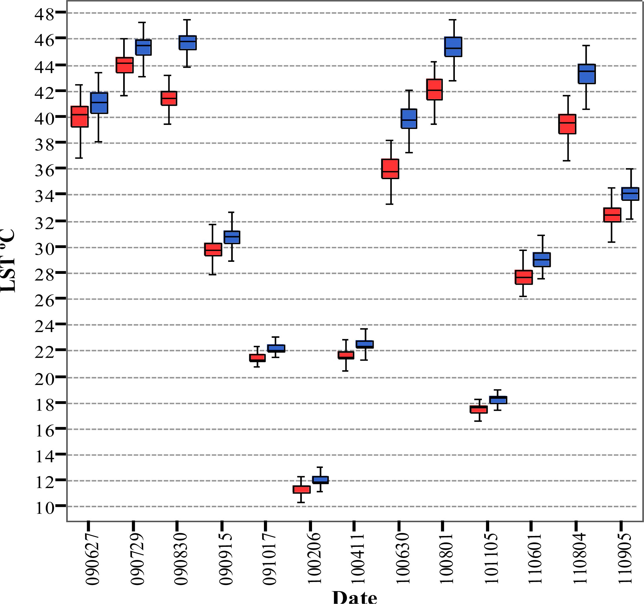
When SC results (the closest to the LST_ref) are compared to MODIS LST, a seasonal bias is observed: the greatest variances (above 6 °C) occur in summer (

Table 9. Differences between LST retrieved from Landsat using MW and SC methods and LST from MODIS MOD11_L2 product.

Date	LSTMODIS (°C)	LSTLandsat–LSTMODIS (°C)
		MW	SC	RTE−ACPC
27/06/2009	39.87	2.05	3.92	5.04
29/07/2009	39.21	4.74	6.11	6.15
30/08/2009	38.87	2.24	6.57	3.28
15/09/2009	28.03	1.75	2.72	3.22
17/10/2009	22.23	−0.38	0.36	−0.90
06/02/2010	11.99	−0.72	0.05	0.00
11/04/2010	22.35	−0.74	0.10	−0.18
30/06/2010	34.17	2.06	5.97	7.23
01/08/2010	39.51	1.98	5.25	3.45
05/11/2010	18.41	−0.92	−0.16	−0.63
01/06/2011	25.27	2.49	3.82	2.70
04/08/2011	38.55	1.84	5.72	6.30
05/09/2011	29.29	3.50	5.09	5.28
Bias		1.53	3.50	3.15
St. Dev		1.74	2.59	2.82

) and the lowest (0.00–0.38 °C) in winter and autumn. This fact was already mentioned in other studies [51]. Trigo et al. [65] observed that greater LST dispersion in summer can be related to the great thermal contrasts between landcover components (bareground, grass, tree canopy) taking place during this season. Because of higher spatial resolution and higher variability in emissivity, Landsat is more sensitive to this dispersion. Greater thermal range of around 8 °C on summer dates can be appreciated in Figure 4 showing Landsat LST variability within MODIS pixel. We should also consider that MODIS surface emissivity estimation is based on landcover types from the map updated annually [69], while NDVI Thresholds emissivity algorithm used in this study is based on NDVI (see Section 2.4).

Another explanation for the magnitude of LST_Landsat–LST_MODIS is the greater spatial and temporal variability of emissivity values estimated from Landsat-5 TM NDVI. This wider range is caused by the higher spatial resolution of the Landsat-5 TM, different algorithms used for emissivity estimation for two sensors and differences in viewing angles between Landsat and MODIS Terra (almost nadiral for Landsat vs. around 60° viewing angles for MODIS Terra) resulting in greater sensitivity of Landsat to an increase in the soil component and greater temperature contrasts between areas with and without vegetation, characteristic to summer as a consequence of grass senescence.

5. Conclusions

The study demonstrates that LST of dehesa ecosystem can be estimated from Landsat-5 TM thermal band using SC and RTE-ACPC procedures with RMSDs lower than 1 °C and the RMSD of 2.3 °C using MW algorithm, with expected uncertainties in energy fluxes modeling of around 10–30 W·m² for SC and RTE-ACPC [17]. The differences with the reference LSTs (LST_ref) are due to the fact that the tested methods are based on the different versions of the radiative transfer code: LOWTRAN 7 for MW and MODTRAN 4 for SC and RTE-ACPC. Moreover, there is a seasonal bias in the MW results, as evident from the correlations between MW-LST_ref and near-surface air temperature and atmospheric water vapor w (R = 0.8), explained by the worse fit of MW coefficients to real atmospheric conditions in the study area compared to other procedures. This dependence is not evident in the LSTs obtained by the SC and RTE-ACPC procedures.

On the other hand, the existing LST mismatch between Landsat and MODIS is due mainly to (1) the time differences in the satellites overpasses and (2) the differences in the viewing angles which make Landsat much more sensitive to changes in the proportion of different landcover components with high thermal contrasts (soil and vegetation) and decrease of emissivity, especially during hot summer months.

Considering the generally-accepted error at the level of 1–2 K [70,71], the three tested procedures (SC, RTE-ACPC, and MW) can be used for LST estimation from Landsat-5 TM thermal data. RMSDs obtained for SC and RTE-ACPC procedures are below 1 °C, with the best results for SC (RMSD = 0.5 °C). This algorithm, which does not require radiosounding data, is considered the most adequate for integration with LST from MODIS MOD11_L2 product. However, the between-sensors differences due to time mismatch and observation angles should be taken into account. It was not possible to estimate the precise magnitude of Landsat-MODIS LST differences due to the lack of information on the contribution of each of the landcover components to ensemble radiance from heterogeneous and non-isothermal pixel characteristic for dehesa ecosystem.

References

- Quattrochi, D.A.; Luvall, J.C. Thermal Remote Sensing in Land Surface Processing; CRC Press: Boca Raton, FL, USA, 2004. [Google Scholar]
- Kustas, W.; Anderson, M. Advances in thermal infrared remote sensing for land surface modeling. Agric. For. Meteorol 2009, 149, 2071–2081. [Google Scholar]
- Zhan, X.; Kustas, W.P.; Humes, K.S. An intercomparison study on models of sensible heat flux over partial canopy surfaces with remotely sensed surface temperature. Remote Sens. Environ 1996, 58, 242–256. [Google Scholar]
- Jia, L.; Menenti, M.; Su, Z.B.; Li, Z.-L.; Djepa, V.; Wang, J.M. Modeling Sensible Heat Flux Using Estimates of Soil and Vegetation Temperatures: The HEIFE and IMGRASS Experiments. In Remote Sensing and Climate Modeling: Synergies and Limitations; Beniston, M., Verstraete, M., Eds.; Kluwer Academic Publishers: Berlin, Germany, 2001; pp. 23–49. [Google Scholar]
- Kalma, J.; McVicar, T.; McCabe, M. Estimating land surface evaporation: A review of methods using remotely sensed surface temperature data. Surv. Geophys 2008, 29, 421–469. [Google Scholar]
- Moran, M.S.; Rahman, A.F.; Washburne, J.C.; Goodrich, D.C.; Weltz, M.A.; Kustas, W.P. Combining the Penman-Monteith equation with measurements of surface temperature and reflectance to estimate evaporation rates of semiarid grassland. Agric. For. Meteorol 1996, 80, 87–109. [Google Scholar]
- Gamon, J.A.; Huemmrich, K.F.; Peddle, D.R.; Chen, J.; Fuentes, D.; Hall, F.G.; Kimball, J.S.; Goetz, S.; Gu, J.; McDonald, K.C.; et al. Remote sensing in BOREAS: Lessons learned. Remote Sens. Environ 2004, 89, 139–162. [Google Scholar]
- Li, Z.-L.; Tang, B.-H.; Wu, H.; Ren, H.; Yan, G.; Wan, Z.; Trigo, I.F.; Sobrino, J.A. Satellite-derived land surface temperature: Current status and perspectives. Remote Sens. Environ 2013, 131, 14–37. [Google Scholar]
- Berk, A.; Anderson, G.P.; Acharya, P.K.; Shettle, E.P. Modtran 5.2.1 User’s Manual; Spectral Sciences, Inc. & Air Force Research Laboratory: Burlington, MA, USA, 2011. [Google Scholar]
- Barsi, J.A.; Barker, J.L.; Schott, J.R. An Atmospheric Correction Parameter Calculator for a Single Thermal Band Earth-Sensing Instrument. Processdings of the 2003 IEEE International Geoscience and Remote Sensing Symposium. IGARSS ’03, Melbourne, Australia, 21–25 July 2003; 5, pp. 3014–3016.
- Barsi, J.A.; Schott, J.R.; Palluconi, F.D.; Hook, S.J. Validation of a web-based atmospheric correction tool for single thermal band instruments. Proc. SPIE 2005. [Google Scholar] [CrossRef]
- Precipitable Water at the VLA—1990–1998. Available online: http://legacy.nrao.edu/alma/memos/html-memos/alma237/memo237.html (accessed on 5 May 2014).
- MODIS Website. Available online: http://modis.gsfc.nasa.gov (accessed on 5 May 2014).
- SEVIRI Sensor WDC-RSAT. Available online: http://wdc.dlr.de/sensors/seviri (accessed on 5 May 2014).
- Landsat Missions. Available online: http://landsat.usgs.gov (accessed on 5 May 2014).
- Landsat 8 (L8) Operational Land Imager (OLI) and Thermal Infrared Sensor (TIRS). Available online: http://landsat.usgs.gov/calibration_notices.php (accessed on 5 May 2014).
- Tang, H.; Li, Z.-L. Introduction. In Quantitative Remote Sensing in Thermal Infrared; Springer: Berlin/Heidelberg, Germany, 2014; pp. 1–4. [Google Scholar]
- Cristóbal, J.; Jiménez-Muñoz, J.C.; Sobrino, J.A.; Ninyerola, M.; Pons, X. Improvements in land surface temperature retrieval from the Landsat series thermal band using water vapor and air temperature. J. Geophys. Res 2009, 114. [Google Scholar] [CrossRef]
- Jimenez-Munoz, J.C.; Cristobal, J.; Sobrino, J.A.; Soria, G.; Ninyerola, M.; Pons, X. Revision of the single-channel algorithm for land surface temperature retrieval from Landsat thermal-infrared data. IEEE Trans. Geosci. Remote Sens 2009, 47, 339–349. [Google Scholar]
- Jiménez-Muñoz, J.C.; Sobrino, J.A. A generalized single-channel method for retrieving land surface temperature from remote sensing data. J. Geophys. Res 2004, 108, 46–88. [Google Scholar]
- Qin, Z.; Karnieli, A.; Berliner, P. A mono-window algorithm for retrieving land surface temperature from Landsat TM data and its application to the Israel-Egypt border region. Int. J. Remote Sens 2001, 22, 3719–3746. [Google Scholar]
- Li, Z.-L.; Wu, H.; Wang, N.; Qiu, S.; Sobrino, J.A.; Wan, Z.; Tang, B.-H.; Yan, G. Land surface emissivity retrieval from satellite data. Int. J. Remote Sens 2013, 34, 3084–3127. [Google Scholar]
- Olioso, A. Simulating the relationship between thermal emissivity and the normalized difference vegetation index. Int. J. Remote Sens 1995, 16, 3211–3216. [Google Scholar]
- Rubio, E.; Caselles, V.; Badenas, C. Emissivity measurements of several soils and vegetation types in the 8–14 μm wave band: Analysis of two field methods. Remote Sens. Environ 1997, 59, 490–521. [Google Scholar]
- Sobrino, J.A.; Raissouni, N. Toward remote sensing methods for land cover dynamic monitoring: Application to Morocco. Int. J. Remote Sens 2000, 21, 353–366. [Google Scholar]
- Valor, E.; Caselles, V. Mapping land surface emissivity from NDVI: Application to European, African, and South American areas. Remote Sens. Environ 1996, 57, 167–184. [Google Scholar]
- Van de Griend, A.A.; Owe, M. On the relationship between thermal emissivity and the normalized difference vegetation index for natural surfaces. Int. J. Remote Sens 1993, 14, 1119–1131. [Google Scholar]
- BIOSPEC. Available online: http://www.lineas.cchs.csic.es/biospec (accessed on 5 May 2014).
- FLUXPEC. Available online: http://www.lineas.cchs.csic.es/fluxpec (accessed on 5 May 2014).
- Agam, N.; Kustas, W.P.; Anderson, M.C.; Li, F.; Neale, C.M. A vegetation index based technique for spatial sharpening of thermal imagery. Remote Sens. Environ 2007, 107, 545–558. [Google Scholar]
- Walker, J.J.; De Beurs, K.M.; Wynne, R.H.; Gao, F. Evaluation of landsat and MODIS data fusion products for analysis of dryland forest phenology. Remote Sens. Environ 2012, 117, 381–393. [Google Scholar]
- Cleugh, H.A.; Leuning, R.; Mu, Q.; Running, S.W. Regional evaporation estimates from flux tower and modis satellite data. Remote Sens. Environ 2007, 106, 285–304. [Google Scholar]
- Copertino, V.A.; Di Pietro, M.; Scavone, G.; Telesca, V. Comparison of algorithms to retrieve land surface temperature from Landsat-7 ETM+ IR data in the Basilicata Ionian band. Tethys 2012, 9, 25–34. [Google Scholar]
- Sobrino, J.A.; Jiménez-Muñoz, J.C.; Paolini, L. Land surface temperature retrieval from Landsat TM 5. Remote Sens. Environ 2004, 90, 434–440. [Google Scholar]
- Baldocchi, D.; Falge, E.; Gu, L.; Olson, R.; Hollinger, D.; Running, S.; Anthony, P.; Bernhofer, C.; Davis, K.; Evans, R.; et al. FLUXNET: A new tool to study the temporal and spatial variability of ecosystem-scale carbon dioxide, water vapor and energy flux densities. Bull. Am. Meteorol. Soc 2001, 82, 2415–2434. [Google Scholar]
- Núñez Corchero, M.; Sosa Cardo, J.A. Climatología de Extremadura (1961–1990); Ministerio de Medio Ambiente: Madrid, Spain, 2001. [Google Scholar]
- USGS Global Visualization Viewer. Available online: http://glovis.usgs.gov (accessed on 5 May 2014).
- Wan, Z.; Dozier, J. A generalized split-window algorithm for retrieving land-surface temperature from space. IEEE Trans. Geosci. Remote Sens 1996, 34, 892–905. [Google Scholar]
- Li, H.; Liu, Q.; Zhong, B.; Du, Y.; Wang, H.; Wang, Q. A. Single-Channel Algorithm for Land Surface Temperature Retrieval from HJ-1B/IRS Data Based on a Parametric Model. Proceedings of the 2010 IEEE International Geoscience and Remote Sensing Symposium (IGARSS), Honolulu, HI, USA, 25–30 July 2010; pp. 2448–2451.
- Noyes, E.; Good, S.; Corlet, G.; Kong, X.; Remedios, J.; Llewellyn-Jones, D. AATSR LST Product Validation. Proceedings of the Second Working Meeting on MERIS and AATSR Calibration and Geophysical Validation (MAVT-2006), Frascati, Italy, 20–24 March 2006.
- Aerosol Robotic Network (AERONET). Available online: http://aeronet.gsfc.nasa.gov (accessed on 5 May 2014).
- Kistler, R.; Kalnay, E.; Collins, W.; Saha, S.; White, G.; Woollen, J.; Chelliah, M.; Ebisuzaki, W.; Kanamitsu, M.; Kousky, V.; et al. The NCEP-NCAR 50-Year Reanalysis: Monthly Means CD-ROM and Documentation; American Meteorological Society: Boston, MA, USA, 2001. [Google Scholar]
- NCEP/NCAR Reanalysis Monthly Means and Other Derived Variables. Available online: http://www.esrl.noaa.gov/psd/data/gridded/data.ncep.reanalysis.derived.surface.html (accessed on 5 May 2014).
- NASA Land Data Service and Products. Available online: https://lpdaac.usgs.gov/get_data/data_pool (accessed on 5 May 2014).
- ENVI Software. Available online: http://www.exelisvis.com/ProductsServices/ENVI/ENVI.aspx (accessed on 5 May 2014).
- Atmospheric Correction Parameter Calculator. Available online: http://atmcorr.gsfc.nasa.gov (accessed on 5 May 2014).
- Sobrino, J.A.; Coll, C.; Caselles, V. Atmospheric correction for land surface temperature using NOAA-11 AVHRR channels 4 and 5. Remote Sens. Environ 1991, 38, 19–34. [Google Scholar]
- Coll, C.; Valor, E.; Galve, J.M.; Mira, M.; Bisquert, M.; García-Santos, V.; Caselles, E.; Caselles, V. Long-term accuracy assessment of land surface temperatures derived from the Advanced Along-Track Scanning Radiometer. Remote Sens. Environ 2012, 116, 211–225. [Google Scholar]
- Wan, Z.; Li, Z.L. Radiance-based validation of the v5 MODIS land-surface temperature product. Int. J. Remote Sens 2008, 29, 5373–5395. [Google Scholar]
- Coll, C.; Caselles, V.; Valor, E.; Niclòs, R. Comparison between different sources of atmospheric profiles for land surface temperature retrieval from single channel thermal infrared data. Remote Sens. Environ 2012, 117, 199–210. [Google Scholar]
- Jiménez-Muñoz, J.C.; Sobrino, J.A.; Mattar, C.; Franch, B. Atmospheric correction of optical imagery from MODIS and Reanalysis atmospheric products. Remote Sens. Environ 2010, 114, 2195–2210. [Google Scholar]
- Gillespie, A.; Rokugawa, S.; Matsunaga, T.; Cothern, J.S.; Hook, S.; Kahle, A.B. A temperature and emissivity separation algorithm for advanced spaceborne thermal emission and reflection radiometer (ASTER) images. IEEE Trans. Geosci. Remote Sens 1998, 36, 1113–1126. [Google Scholar]
- Becker, F.; Li, Z.-L. Temperature-independent spectral indices in thermal infrared bands. Remote Sens. Environ 1990, 32, 17–33. [Google Scholar]
- Sobrino, J.A.; Raissouni, N.; Li, Z.-L. A comparative study of land surface emissivity retrieval from NOAA data. Remote Sens. Environ 2001, 75, 256–266. [Google Scholar]
- Sobrino, J.A.; Jiménez-Muñoz, J.C.; Soria, G.; Romaguera, M.; Guanter, L.; Moreno, J.; Plaza, A.; Martinez, P. Land surface emissivity retrieval from different VNIR and TIR sensors. IEEE Trans. Geosci. Remote Sens 2008, 46, 316–327. [Google Scholar]
- Choudhury, B.J.; Ahmed, N.U.; Idso, S.B.; Reginato, R.J.; Daughtry, C.S.T. Relations between evaporation coefficients and vegetation indices studied by model simulations. Remote Sens. Environ 1994, 50, 1–17. [Google Scholar]
- Gutman, G.; Ignatov, A. The derivation of the green vegetation fraction from NOAA/AVHRR data for use in numerical weather prediction models. Int. J. Remote Sens 1998, 19, 1533–1543. [Google Scholar]
- Kneizys, F.X.; Shettle, E.; Abreu, L.; Chetwynd, J.; Anderson, G. Users Guide to LOWTRAN 7; Air Force Geophysics Lab Hanscom AFB: Saugus, MA, USA, 1988. [Google Scholar]
- Berk, A.; Anderson, G.P.; Bernstein, L.S.; Acharya, P.K.; Dothe, H.; Matthew, M.W.; Adler-Golden, S.M.; Chetwynd, J.H., Jr.; Richtsmeier, S.C.; Pukall, B. Modtran4 Radiative Transfer Modeling for Atmospheric Correction. Proceedings of the International Society for Optics and Photonics SPIE’s International Symposium on Optical Science, Engineering, and Instrumentation, Denver, CO, USA, 18 July 1999; pp. 348–353.
- Zhao, L.; Tian, Q.; Wan, W.; Yu, T.; Gu, X.; Chen, H. Atmospheric Sensitivity on Land Surface Temperature Retrieval Using Single Channel Thermal Infrared Remote Sensing Data: Comparison among Models. Proceedings of the 2010 18th International Conference on Geoinformatics, Beijing, China, 18–20 June 2010; pp. 1–6.
- Schmugge, T.; Hook, S.J.; Coll, C. Recovering surface temperature and emissivity from thermal infrared multispectral data. Remote Sens. Environ 1998, 65, 121–131. [Google Scholar]
- Srivastava, P.K.; Majumdar, T.J.; Bhattacharya, A.K. Surface temperature estimation in Singhbhum Shear zone of India using Landsat-7 ETM+ thermal infrared data. Adv. Space Res 2009, 43, 1563–1574. [Google Scholar]
- Qian, Y.-G.; Li, Z.-L.; Nerry, F. Evaluation of land surface temperature and emissivities retrieved from MSG/SEVIRI data with MODIS land surface temperature and emissivity products. Int. J. Remote Sens 2012, 34, 3140–3152. [Google Scholar]
- Soria, G.; Sobrino, J.A.; Atitar, M.; Jiménez-Muñoz, J.C.; Hidalgo, V.; Julien, Y.; Ruescas, A.B.; Franch, B.; Mattar, C.; Oltra, R. AATSR Land Surface Temperature Product: Comparison with SEVIRI and MODIS in the Framework of CEFLES2 Campaigns. Proceedings of the 2nd MERIS/AATSR User Workshop, Frascati, Italy, 22–26 September 2008; 2008. [Google Scholar]
- Trigo, I.F.; Monteiro, I.T.; Olesen, F.; Kabsch, E. An assessment of remotely sensed land surface temperature. J. Geophys. Res. Atmos 2008, 113. [Google Scholar] [CrossRef]
- Li, F.; Jackson, T.J.; Kustas, W.P.; Schmugge, T.J.; French, A.N.; Cosh, M.H.; Bindlish, R. Deriving land surface temperature from Landsat 5 and 7 during SMEX02/SMACEX. Remote Sens. Environ 2004, 92, 521–534. [Google Scholar]
- Rasmussen, M.O.; Pinheiro, A.C.; Proud, S.R.; Sandholt, I. Modeling angular dependences in land surface temperatures from the seviri instrument onboard the geostationary Meteosat second generation satellites. IEEE Trans. Geosci. Remote Sens 2010, 48, 3123–3133. [Google Scholar]
- Hesslerová, P.; Pokorný, J.; Brom, J.; Rejšková-Procházková, A. Daily dynamics of radiation surface temperature of different land cover types in a temperate cultural landscape: Consequences for the local climate. Ecol. Eng 2013, 54, 145–154. [Google Scholar]
- Snyder, W.C.; Wan, Z.; Zhang, Y.; Feng, Y.Z. Classification-based emissivity for land surface temperature measurement from space. Int. J. Remote Sens 1998, 19, 2753–2774. [Google Scholar]
- French, A.N.; Norman, J.M.; Anderson, M.C. A simple and fast atmospheric correction for spaceborne remote sensing of surface temperature. Remote Sens. Environ 2003, 87, 326–333. [Google Scholar]
- Sobrino, J.A.; Frate, F.; Drusch, M.; Jiménez-Muñoz, J.C.; Manunta, P. Review of High Resolution Thermal Infrared Applications and Requirements: The FUEGOSAT Synthesis Study. In Thermal Infrared Remote Sensing; Kuenzer, C., Dech, S., Eds.; Springer: Dordrecht, The Netherlands, 2013; pp. 197–214. [Google Scholar]