The Improved NRL Tropical Cyclone Monitoring System with a Unified Microwave Brightness Temperature Calibration Scheme

Abstract
: The near real-time NRL global tropical cyclone (TC) monitoring system based on multiple satellite passive microwave (PMW) sensors is improved with a new inter-sensor calibration scheme to correct the biases caused by differences in these sensor’s high frequency channels. Since the PMW sensor 89 GHz channel is used in multiple current and near future operational and research satellites, a unified scheme to calibrate all satellite PMW sensor’s ice scattering channels to a common 89 GHz is created so that their brightness temperatures (TBs) will be consistent and permit more accurate manual and automated analyses. In order to develop a physically consistent calibration scheme, cloud resolving model simulations of a squall line system over the west Pacific coast and hurricane Bonnie in the Atlantic Ocean are applied to simulate the views from different PMW sensors. To clarify the complicated TB biases due to the competing nature of scattering and emission effects, a four-cloud based calibration scheme is developed (rain, non-rain, light rain, and cloudy). This new physically consistent inter-sensor calibration scheme is then evaluated with the synthetic TBs of hurricane Bonnie and a squall line as well as observed TCs. Results demonstrate the large TB biases up to 13 K for heavy rain situations before calibration between TMI and AMSR-E are reduced to less than 3 K after calibration. The comparison stats show that the overall bias and RMSE are reduced by 74% and 66% for hurricane Bonnie, and 98% and 85% for squall lines, respectively. For the observed hurricane Igor, the bias and RMSE decrease 41% and 25% respectively. This study demonstrates the importance of TB calibrations between PMW sensors in order to systematically monitor the global TC life cycles in terms of intensity, inner core structure and convective organization. A physics-based calibration scheme on TC’s TB corrections developed in this study is able to significantly reduce the biases between different PMW sensors.
1. Introduction
Severe weather phenomena such as tropic cyclones (TC), especially intense TCs, can bring dramatic damages to societies, properties and human lives. For example, hurricane Katrina in August 2005 killed 1883 people and caused an estimated property damage of 81 billion dollars, while Hurricane Sandy in October 2012 led to loss of 285 lives and property damage of 68 billion [1,2]. Although more accurate TC track and intensity forecasts via numerical weather prediction (NWP) models is key to helping governmental agencies and private organizations more effectively prepare for approaching TCs enhanced monitoring of the TC’s initial conditions is crucial to near real-time TC warning efforts. Since most TCs originate in tropical oceans and spend the majority of their life span over data sparse regions, space-based instruments are often the only available platform to monitor a TC’s life cycle when factoring in both the spatial and temporal scales required. Geostationary (GEO) satellites have excellent temporal and spatial resolution sampling attributes, however, GEO infrared (IR)/visible (VIS) channels are not able to provide consistently accurate location and intensity estimates due to their inability to see through upper-level clouds. The TC low-level circulation center is often shielded by a central dense overcast (CDO) frequently limiting the Dvorak technique’s method of analyzing cloud, rainband and eyewall organization, thus causing inherent inaccuracies. The passive microwave (PMW) imager channels onboard low earth orbiting (LEO) satellites observe radiances from both the Earth’s surface and cloud emissions as well as scattering by ice particles associated with intense convection (eyewall and rainbands). The large brightness temperature (TB) depressions caused by ice scattering at 85–91 GHz (40–60 K) provides excellent all-weather views of storm rainband organization and inner core structure that is highly correlated with storm intensity [3–5].
The high frequency (85–91 GHz) PMW sensor channels are a suitable choice for monitoring TC location, structure, and intensity because of their ability to penetrate clouds and mitigate VIS/IR deficiencies and their modest spatial resolution (5–13 km). Three to five channels of LEO PMW sensors are normally available at 10, 19, 23, 37, and 85 or 89/91 GHz and both vertical and horizontal polarizations are usually utilized. The low frequency channels are for measuring emission signals from the surface and atmosphere, while the high frequency channels measure the suppressed TB due to the scattering effects of ice particles [6–9]. In general, convective clouds associated with TCs have many frozen hydrometeors above the freezing level (∼4500 m) and they scatter the energy in the 85–91 GHz channels, thus depressing the signal received by the LEO PMW sensor above. The observed TB depression is a function of the number and size of the frozen hydrometeors; thus, intense convection that reaches higher altitudes (eyewall and intense rainband convection) is readily monitored by PMW sensors [3–5,10]. Since the PMW high frequency channel at horizontal polarization can depict better TC horizontal structures due to a high sensitivity of surface emissivity at H-polarization, the H-polarization high frequency channel is normally applied for monitoring TC life cycle [3–5].
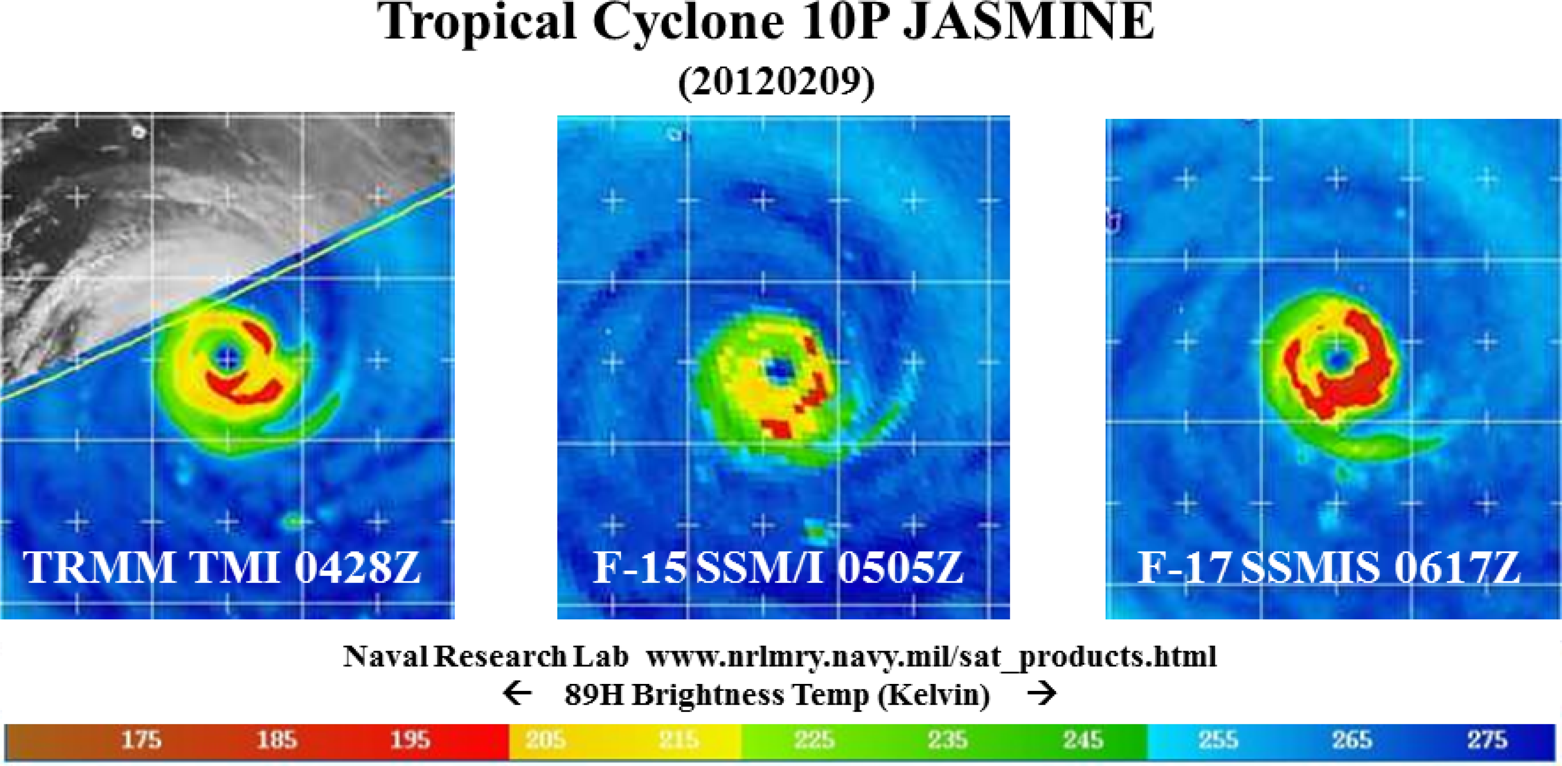
Due to the LEO polar orbits and modest swaths (1300–1700 km), there are only a maximum of two observations per day per satellite over a specific TC, typically less. Thus, a single PMW sensor has insufficient temporal sampling to monitor a TC’s life cycle. However, by using a combination of both operational and research satellite PMW sensors available in near real-time, we are able to globally track the life cycles of TCs in terms of location, intensity, structure, movement, and aspects of rapid intensification (Kieper and Jiang, 2012 [11]). The current PMW constellation consists of the Special Sensor Microwave/Imager (SSM/I) and Special Sensor Microwave Imager Sounder (SSMIS, currently on four spacecraft) on Defense Meteorological Satellite Program (DMSP) satellites, the Navy’s Coriolis WindSat polarimetric radiometer provides both imagery and ocean surface wind vectors, but does not include an ice scattering channel, NASA/JAXA Tropical Rainfall Measuring Mission (TRMM) microwave imager (TMI), JAXA Advanced Microwave Scanning Radiometer 2 (AMSR2) onboard the Global Change Observation Mission 1st-Water (GCOM-W1) satellite, Chinese Fengyun-3 (FY-3) Microwave Radiation Instrument (MWRI), as well as the NASA Global Precipitation Measurement (GPM) microwave imager (GMI). The NASA Advanced Microwave Scanning Radiometer for EOS (AMSR-E) provided high resolution imagery and derived products for nearly a decade before failing in 2011. By combining these sensors, we typically have an observation every 3–5 hours during a TC’s lifecycle [5]. However, there is a critical issue with this approach, i.e., the high frequency channel (i.e., 85–91 GHz) varies from one series of sensors to another, which leads to inconsistencies in TB fields. For example, SSMI and TMI high frequency channels are at 85 GHz, while SSMIS is at 91 GHz and AMSR-E, AMSR2, MWRI and GMI are at 89 GHz. The high frequency difference of these sensors will lead to different TB for the same TC being sampled. Thus, misleading intensities can occur to a satellite analyst who does not take these factors into account. Figure 1 shows the H-polarization high frequency TB images of TC Jasmine on 9 February 2012 observed by TMI, SSMI and SSMIS. Without a proper sensor calibration, it could be mistakenly considered to encounter weakening followed by intensification, while the truth is that Jasmine was steadily weakening during this time. Thus, it is important to have a proper inter-sensor calibration scheme for monitoring TC life cycle via multiple satellite sensors.
There are many different methods that can be used to calibrate different sensors for weather monitoring or climate studies. Yang et al. [12] applied the simultaneous scanning overpass (SCO) technique to calibrate all SSM/I sensors using F-13 as the baseline for creating the SSM/I climate data records and showed significant impacts of the calibration on climate trend of TB and TB-based total precipitating water path. Berg et al. [13] and Sapiano et al. [14] discussed their procedures of creating a fundamental climate data record (FCDR) using both SSM/I and SSMIS. For climate datasets, removing the intersensor bias is the key issue. However, for weather monitoring, calibration impacts of the frequency shift from different sensors due to different emission and scattering effects of atmosphere is the key target. In this study, we will demonstrate a physically-based unified microwave TB calibration scheme and its impacts on improving the NRL near real-time TC monitoring system.
2. Methodology and Datasets
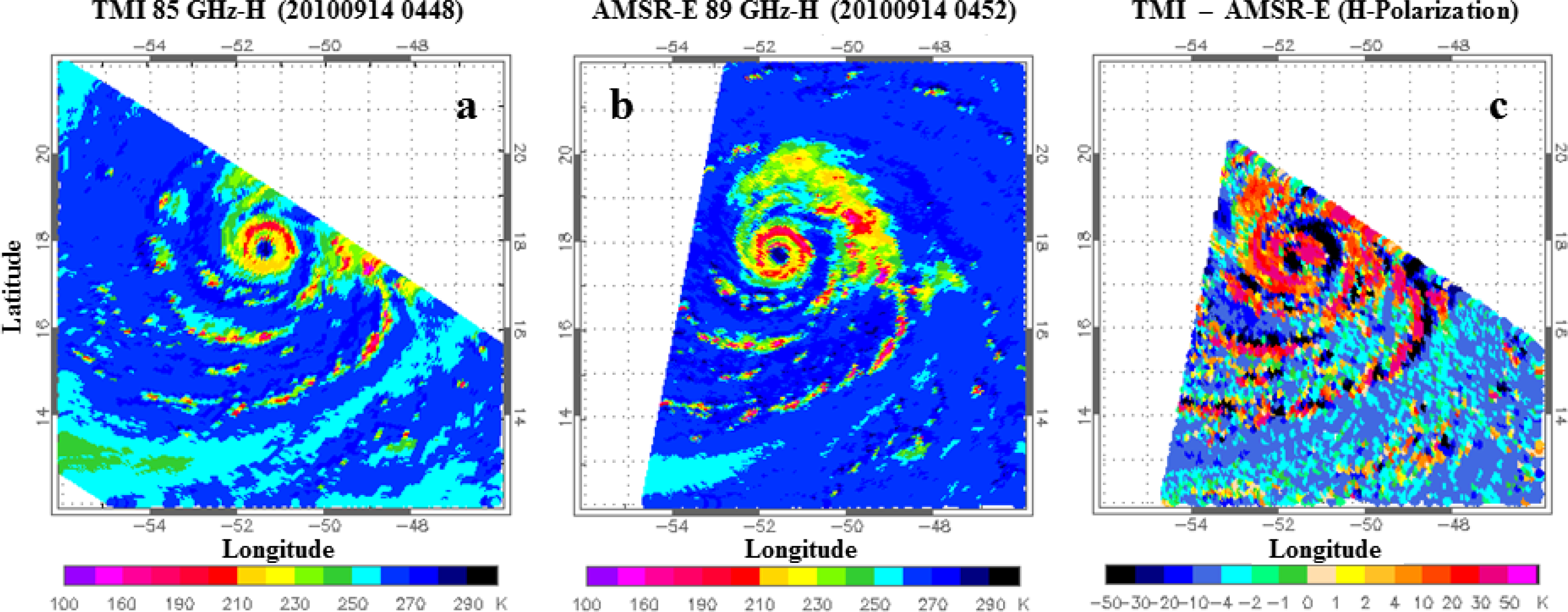
Since recent operational satellite microwave imagers have a high frequency channel at 89 GHz and the GMI also have an 89 GHz channel, a natural choice is to select 89 GHz as the high frequency channel to be used for the calibrated TBs in our global TC monitoring system. Thus, the TBs at 85 or 91 GHz will be recalibrated to 89 GHz. Figure 2 shows an example of the hurricane Igor TB images observed at almost the same time on 14 September 2010 with only a 4-minute difference between TMI at 85H GHz and AMSR-E at 89 GHz. The dramatic TB changes going from a partial red ring at 85 GHz to a complete red ring in 89 GHz in the eyewall would indicate the TC has intensified due to the expansion of intense convective organization in the eyewall, however, it is mainly due to the frequency shift from 85 to 89 GHz as shown in the following Section 3. The right panel is the TB differences for the observed overlapping area. The obvious large TB difference has a similar TC structure pattern, and is due to a combination of TC position movement during the 4 minutes and the 4 GHz frequency difference. Distributions of the maximum TB differences are always near the edge of the TC eyewall and convective spiral areas, indicating the TC movement is the major factor of this large TB difference. In addition, difference in view angle from different PMW sensors will lead to TB difference for a same surface scene. Therefore, the SCO technique is not a good method for intersensor calibration designed for TC monitoring because it is almost impossible to find these pairs of TBs by two different satellite sensors under identical conditions. Because of the strong intensity of TCs, any slight mismatch will lead to a large TB difference. In order to develop a scheme that is physically consistent with different sensors on various satellite platforms, analyses of the synthetic TBs simulated for different sensors under the same atmospheric conditions will lead to a reasonable calibration scheme.
Outputs of the hurricane Bonnie and tropical squall line simulations have thus been utilized to simulate the satellite views of these two weather phenomena. Bonnie was simulated with Mesoscale Modeling system (MM5) and the squall line occurring on 22 February 1993 was simulated with the Goddard Cumulus Ensemble (GCE). Both cases were well simulated and analyzed and also used for databases in TRMM and GPM rain algorithm developments [15,16]. The Community Radiative Transfer Model (CRTM) developed by the Joint Center for Satellite Data Assimilation (JCSDA) is applied to simulate the measurements of satellite sensors such as SSM/I, SSMIS, TMI, and AMSR-E. A total of 90,280 grid data points from hurricane Bonnie and tropical squall line cloud model outputs are simulated with CRTM for TC TB calibrations due to the frequency shift. This simulated dataset involves a large dynamic range of TBs and various cloud systems so that the calibration results based on this dataset should be reliable. With careful analyses of these simulated TBs, calibration coefficients are developed and evaluated with several observed TCs from TMI, AMSR-E and SSMIS.
3. Unified Intersensor Calibration Scheme
3.1. Forward Model Calculations of Cloud Model Simulations
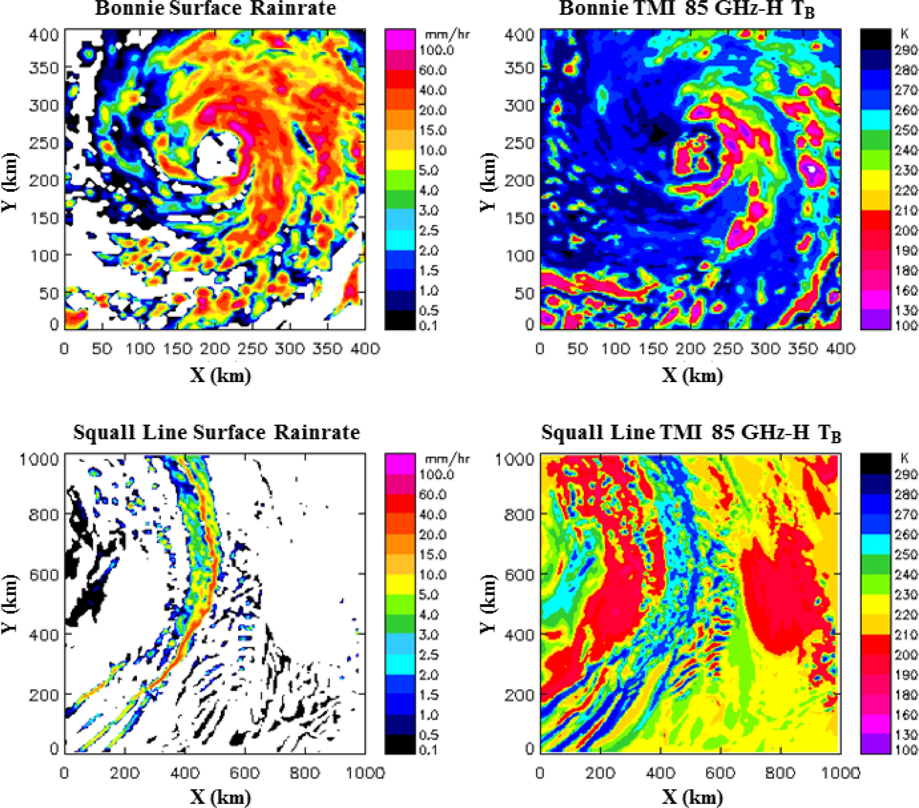
The cloud model outputs of two well-simulated weather systems are used as inputs to the CRTM forward simulations to simulate the satellite views of these storms by different PMW sensors. Thus, the simulated TBs for different sensors are physically consistent for intersensor calibrations. Figure 3 shows the simulated TB at TMI 85 GHz-H and surface rainrate distributions of hurricane Bonnie (top panels) and squall line (bottom panels). Hurricane Bonnie is a well-developed TC with a clear eyewall and spiral convective zones (rainbands). The heavy rain events are concentrated in the east section of this storm and the rainbands. The suppressed TB presents a similar TC pattern due to the scattering effect of ice particles at high frequency. The rainrate map depicts a clear squall line formation and the simulated high frequency TB has a correspondingly suppressed TB along the squall line because of the ice scattering effect associated with strong convection.
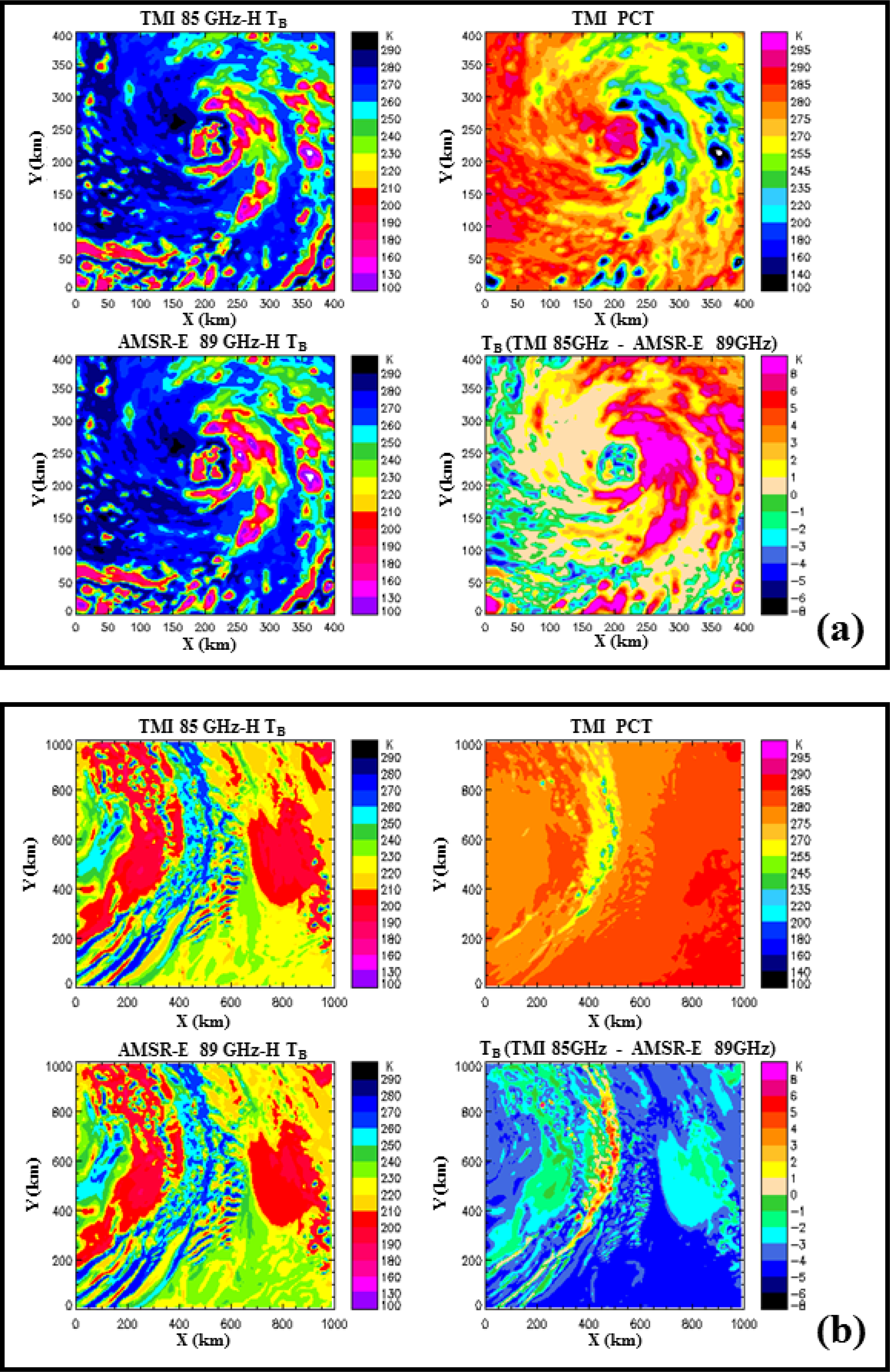
Sometimes it is hard to visually distinguish the TB differences between two sensors because there are not enough colors used in displaying TC images with a fine resolution in resolving those relatively small TBs differences. For example, the simulated TMI 85 GHz-H and AMSR-E 89 GHz-H TB fields for Hurricane Bonnie appear to be quite similar (Figure 4a, left panels). However, their TB differences are actually up to ±10K, shown in the right-bottom panel of Figure 4a. This TB magnitude differences are significant in judging whether a TC is in process of intensification or weakening. A similar spatial pattern of the TB difference and the TC’s rainfall provides a clue for how to calibrate the TB difference associated with the frequency shift. Previous studies already show that the PMW sensor polarization information can be applied to separate the highly polarized radiances of the ocean from essentially unpolarized radiances from precipitation scattering [17,18]. Spencer et al. [9] demonstrated that the polarization corrected temperature (PCT = 1.818TBv − 0.818TBh) can be applied to detect precipitation clouds. Their results indicate a PCT threshold of 255 K for precipitation and 270 K for non-precipitation clouds. The relevant PCT at TMI 85 GHz is shown on the upper-right panel of Figure 4a. It is evident that the PCT pattern is similar to the TC rain map and the correction magnitude is closely linked to the TC convection intensity.
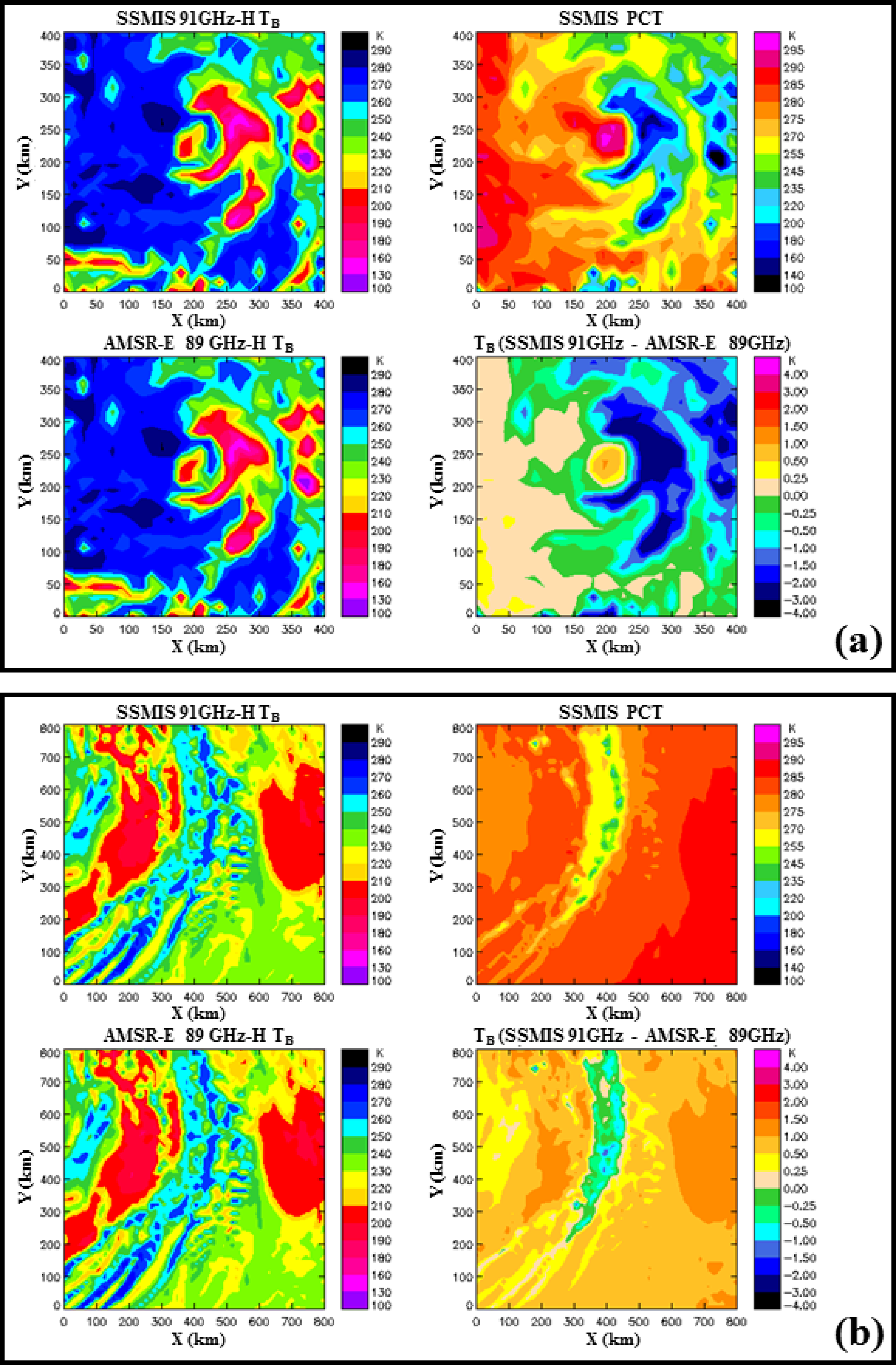
Similar results are found for the squall line case except with a small value of TB corrections because the convection intensity of the squall line is much weaker than hurricane Bonnie (Figure 4b). The positive corrections up to 6K are located at the squall line zone while the negative corrections up to −5K are over the non-rain areas. By the same token, a similar PCT formula, cloud type classification, and analysis are conducted between SSMIS 91 GHz and AMSR-E 89 GHz channels (Figure 5). As expected, similar results are found with smaller TB corrections of ±4K between SSMIS and AMSR-E due to their smaller frequency difference.
3.2. Development of the Intersensor Calibration Scheme
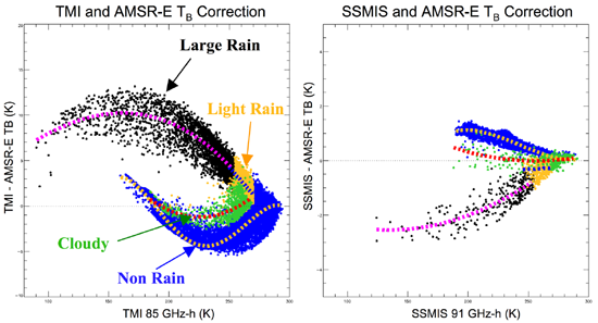
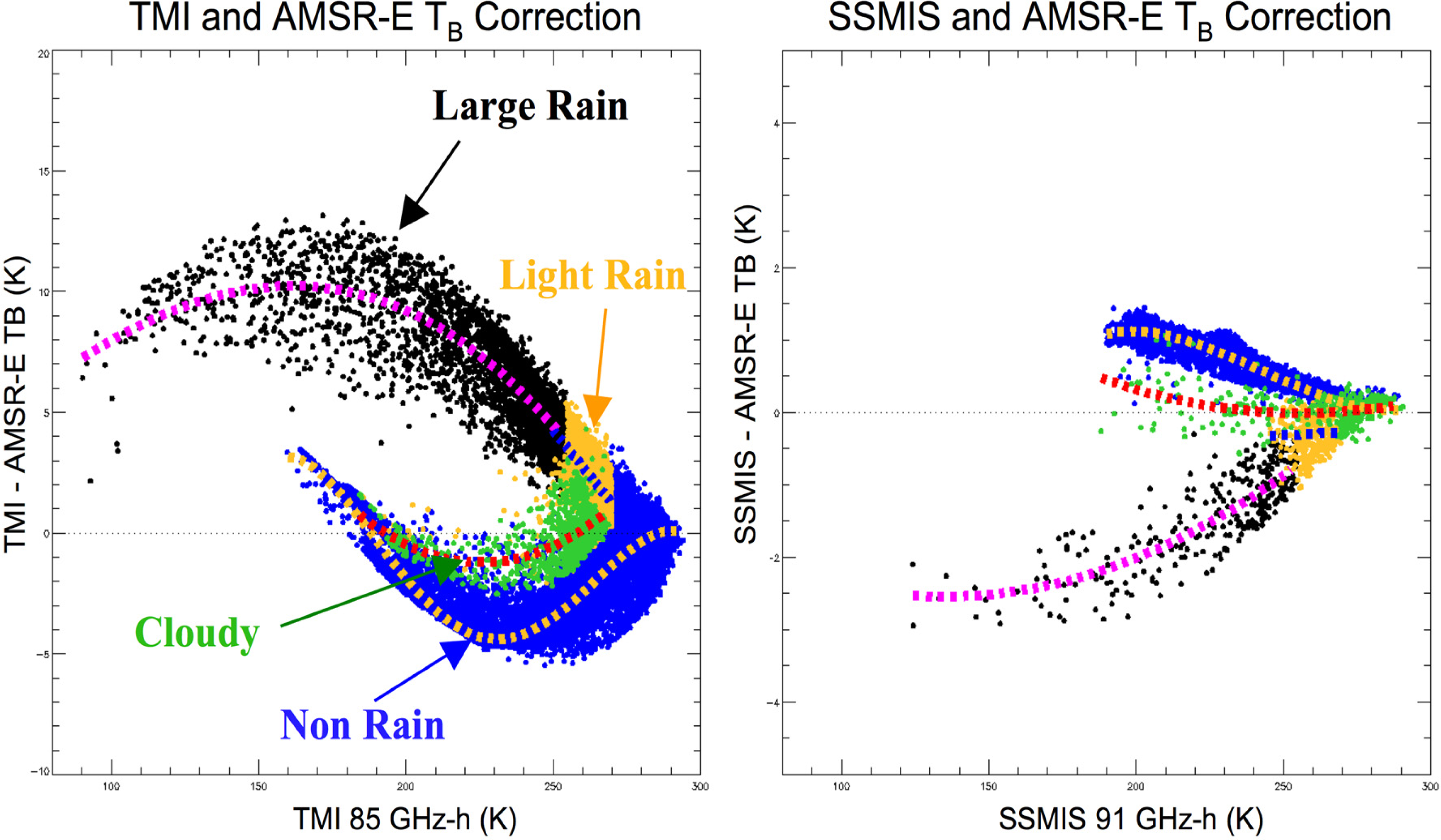
A combination of the simulated TBs from hurricane Bonnie and the squall line cloud model simulations increases the TB dynamic range of weather systems observed by satellite sensors, leading to a calibration scheme more suitable for operational TC monitoring systems. The TB differences of the matched pairs of TMI 85-H GHz and AMSR-E 89-H GHz from the combined datasets are plotted in the left panel of Figure 6. The first impression is that there is a very complicated pattern of the TB differences due to the frequency shift; however, this correction pattern makes sense when considering the physics associated with the combined atmospheric emission and scattering on TBs measured by PMW sensors.
Both emission and scattering effects increase to higher frequencies for PMW sensors. The emission signal will increase TB while the scattering signal will suppress TB. Thus, the final impact on TB will depend on the net effect of emission and scattering. As discussed earlier, the TB correction pattern is similar to the precipitation distribution, thus we have taken an approach of using cloud types to separate different correction patterns so that the physics associated with these corrections are consistent from scene to scene. The four cloud types are classified as non-rain, cloudy, light rain, and large rain. A scene is defined as non-rain when PCTTMI > 270 K. The increased surface emissivity due to the frequency shift from 85 to 89 GHz generally leads to a negative TB correction (blue dots), except a positive correction when TMI 85-H GHz TB is less than 200 K, where non-raining clouds could exist. The magnitude of its TB correction is within ±5. The polynomial fitting is the dashed thick yellow line. The raining scene is when PCTTMI ≤ 255 K (black dots). The mean rainrate of these black dots is 4.85 mm·hr−1. It is obvious the scattering effect of raining particles is greater than the increased emission effect so that the net effect is the suppressed TBs at 89 GHz which leads to a positive TB correction for raining conditions (polynomial fitting is the dashed pink line). The maximum TB corrections could reach 13 K from this scattering plot; however, the final maximum TB correction is only about 10 K from the fitting line.
When 255 K < PCTTMI ≤ 270 K, the scene represents a weak emission and scattering situation so that the correction is relatively small (yellow and green dots). The TB bias correction pattern is still too complex. In order to further separate these data points for a clear TB correction, we apply a scattering index (SI) defined in Yang and Smith [19]. These yellow dots are associated with SI > −25 K, while the green dots are with SI ≤ −25 K. When the suppressed TB effect due to scattering is more than the emission TB contribution, we would expect a positive TB bias for the frequency shift. The majority of these yellow dots with positive TB biases (Figure 6, left panel) provide the evidence that our criterion is reasonable, although there are still a few outliers. The mean rainrate of these yellow dots is 0.28 mm·hr−1. Thus, this scenario is defined as a light rain situation. The green dots are defined as cloudy situations while the dashed red line is a polynomial fitting of the cloudy conditions. In order to properly fit the yellow dots, an additional criterion of TB TMI ≥ 250 K is introduced so that the dashed blue line is their linear fit. By the same token, a similar analysis is conducted for intersensor corrections between SSMIS 91 and AMSR-E 89 GHz. Because of the smaller frequency difference with respect to TMI/AMSR-E, a smaller TB bias is expected. Also, the sign of TB correction patterns would be opposite to that shown in TMI/AMSR-E due to correction from 91 to 89 GHz. The collected pairs of the matched SSMIS 91-H and AMSR-E 89-H GHz dataset are shown in the right panel of Figure 6. It is obvious the sign of correction patterns is opposite as shown in left panel of Figure 6. A similar four cloud classification scheme is applied, i.e., non-rain, large rain, light rain, and cloudy. The non-rain category is defined as PCTssmis > 270 K and a rain index RI19 > 7 K (blue dots). The rain index RI19 defined in Yang and Smith [19] is adapted here. The rain category is defined as PCTssmis ≤ 255 K (black dots). The light rain category is defined as 255 K < PCTSSMIS ≤ 270 K and TBssmis > 245 K (yellow dots), while green dots are for cloudy category when either 255 K < PCTSSMIS ≤ 270 K and TBssmis ≤ 245 K or PCTssmis > 270 K and RI19 ≤ 7 K. Their associated fitting curves are dashed yellow, pink, blue and red lines.
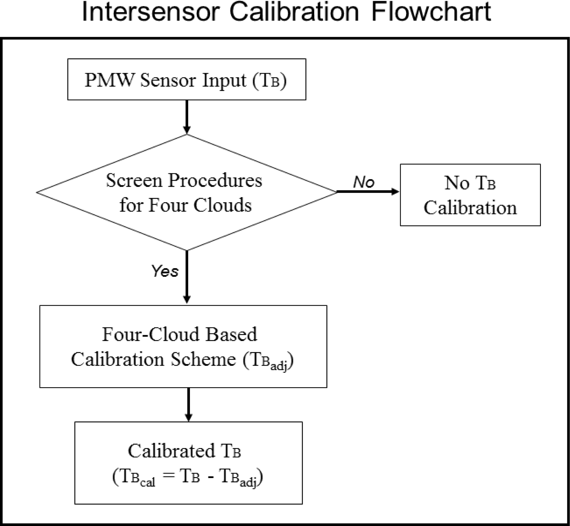
The TMI and SSMIS associated TB calibration coefficients due to their frequency shift to 89-H GHz are listed in Table 1. The flowchart of this unified intersensor calibration scheme is given in Figure 7, highlighting the key processes as the procedures to identify the four cloud categories. Similar processes have been conducted for vertical polarization channels. A similar TB correction curve at V-polarization channels is obvious for rainy clouds, while small differences exist for non-rain clouds due to their small TB dynamic range. The same processes have also been conducted for SSM/I and similar results are omitted in this paper.
4. Calibration Impact on TC Monitoring
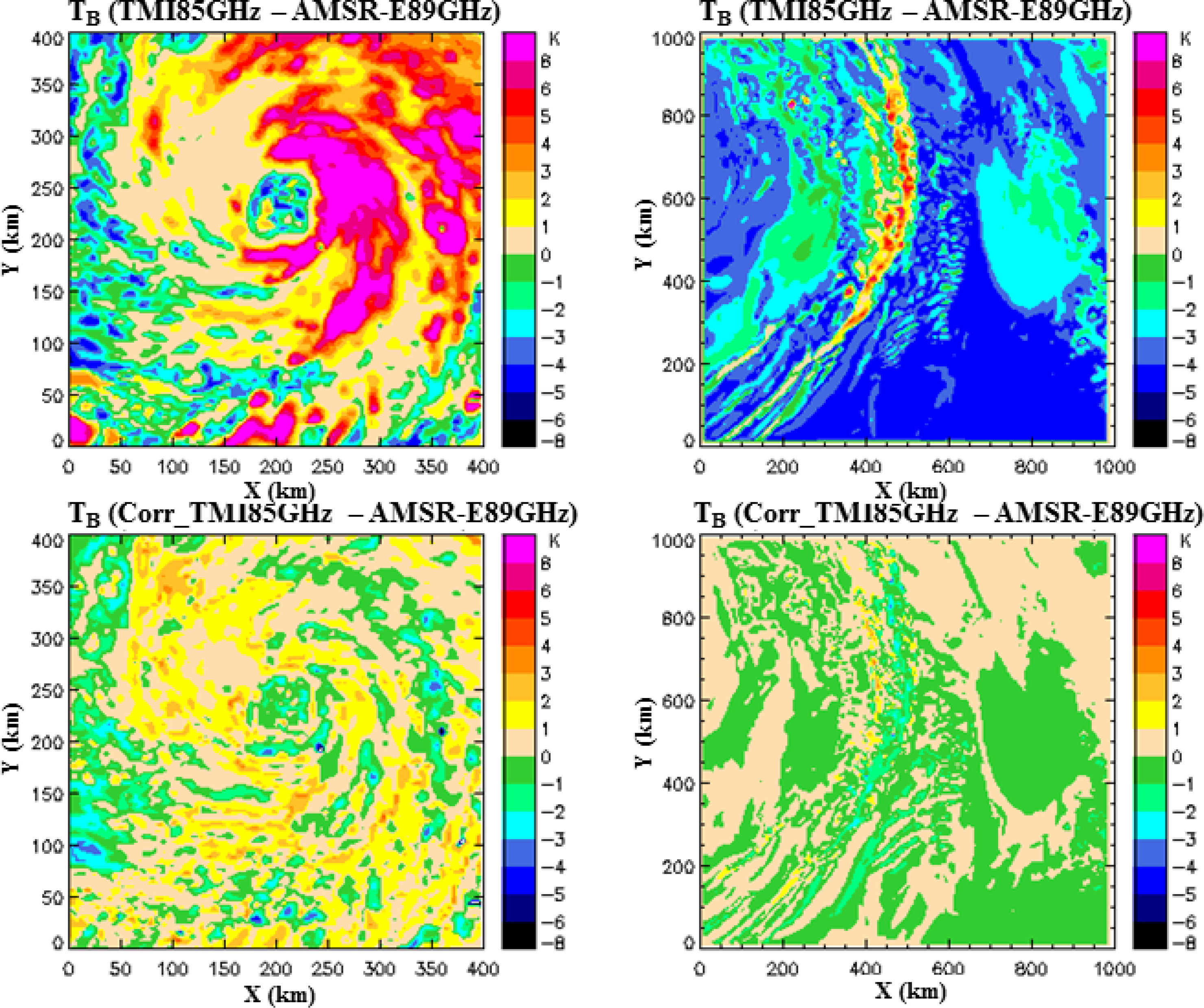
The developed scheme is now evaluated with the synthetic TBs from the two cloud model simulations and observed TCs. Figure 8 (left panels) shows comparisons of the TB differences between TMI 85-H and AMSR-E 89-H GHz for the simulated hurricane Bonnie before and after calibration. The large TB differences due to the mismatched frequency are up to 10K over the TC deep convection areas (upper-left panel). The TB bias pattern is similar to the TC rainfall distribution. With the intersensor calibration, these TB differences are dramatically reduced to within 2K (bottom-left panel). Besides, the bias pattern is no longer mimicking the TC rainfall pattern. Similar results are found with the squall line case (Figure 8, right panels). The decrease of the TB biases over the squall line with the new scheme is significant, although it seems that there is a slight overcorrection. However, the overall reduction of TB differences for the squall line case is prominent with this newly developed intersensor calibration scheme.
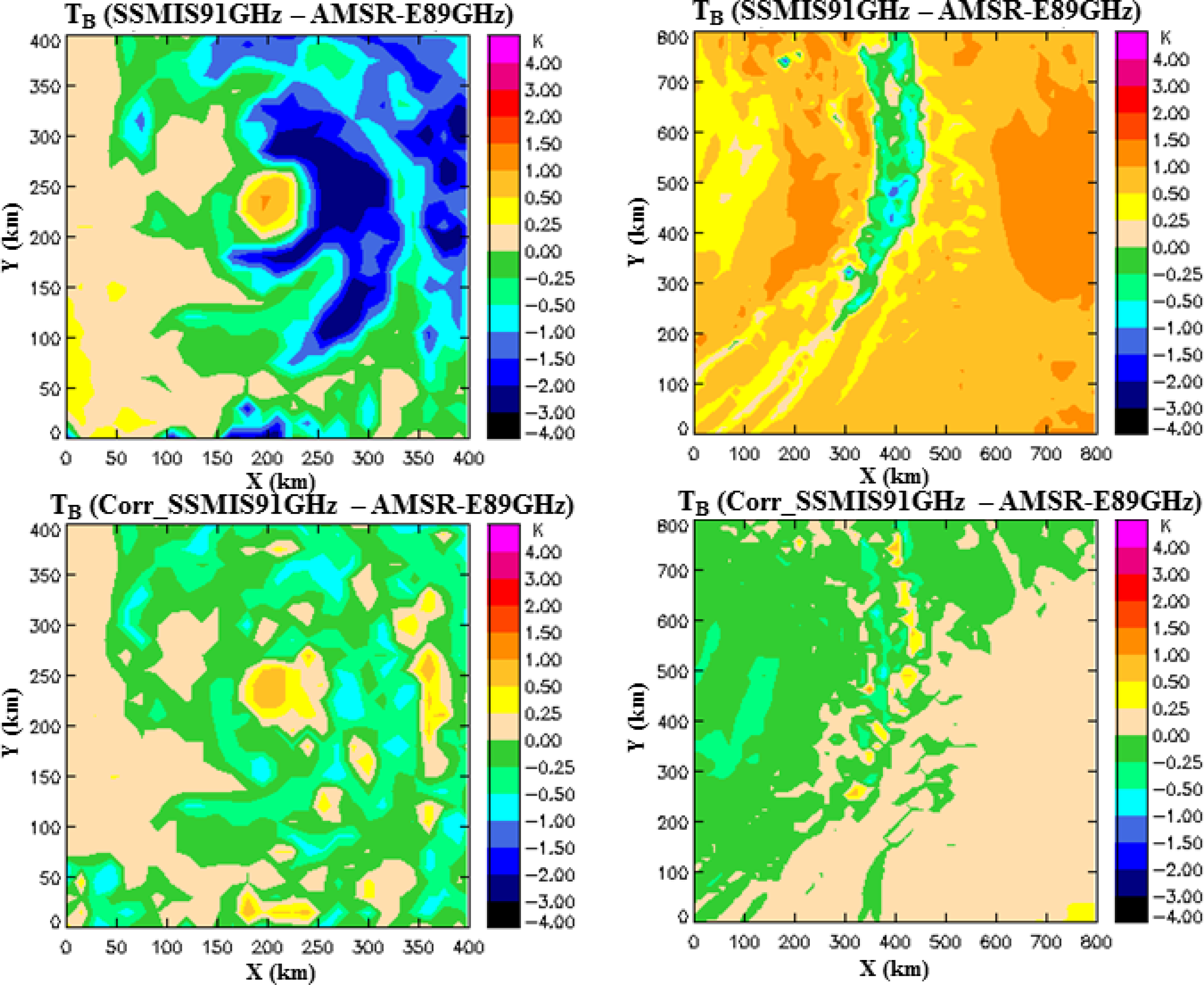
Similar comparisons between SSMIS 91 and AMSR-E 89 GHz-H are presented in Figure 9. It is obvious that their TB differences reduce significantly after application of this new calibration scheme. Table 2 summarizes a few key statistics of comparison between TMI 85 GHz and AMSR-E 89 GHz before and after application of this new calibration scheme. For simulated hurricane Bonnie, the horizontal polarization TB bias before and after calibration is 1.787 K and 0.463 K, respectively, resulting in a bias deduction of 74.1%. The relevant correlation coefficient changes from 0.996 to 0.999, increasing 0.3%. The root mean square error (RMSE) varies from 4.002 K to 1.360 K, decreasing 66%. For the simulated squall line, the TB bias goes from −2.964 K to −0.059 K, a decrease of 98%, while correlation coefficient from 0.997 to 1.000, an increase of 0.3%. RMSE changes from 3.364 K to 0.507 K, a deduction of 84.9%. These results demonstrate the effectiveness of this new scheme in calibrating TB differences between TMI and AMSR-E due to their frequency shift.
The cloud type classification is an important process in the TB calibration scheme; especially the identification of rainy clouds because they are associated with large TB corrections. Fortunately, rainy cloud detection with a PCT index is well established [9]. The scattering index for light rain and cloudy situations could have errors in cloud identifications. However, the impact of misclassifications should be relatively small because of their associated small TB calibrations due to frequency shift. In addition, there are differences of calibration accuracy among various PMW sensors. SSMIS NEdT at 91 GHz is 0.69 K, SSM/I at 85 GHz is 0.69 K (V-pol) and 0.73 K (H-pol). NEdT of TMI at 85 GHz is 0.52 K (V-pol) and 0.97 K (H-pol), while AMSR-E at 91 GHz is less than 1K. Thus, the sensor calibration accuracy difference is generally less than 0.5 K, which is much smaller that the TB difference corrections up to 10K due to frequency shift from 85 to 89 GHz. Therefore, the PMW sensor calibration accuracy difference will not significantly impact the accuracy of TB corrections from frequency shift.
In order to implement this scheme in our near-real time TC monitoring system, we need to evaluate it using observed TCs. Figure 10 shows an example of hurricane Igor on 14 September 2010 between TMI and AMSR-E before and after calibration. The left panels are TBs from TMI 85-H GHz and AMSR-E 89-H GHz before calibration. This is an excellent case because the observing times by TMI and AMSR-E are so close (<4 min) that the intensity change due to TC intensification or decay is insignificant. Thus, their TB differences can be mainly attributed to the sensor’s frequency difference. The right top corner is Igor’s TB correction pattern. The large positive biases are over the precipitating areas while relatively small negative bias is over non-rain and cloudy areas. The TB distribution after calibration of TMI 85 to 89-H GHz is presented on the right bottom panel. It can be seen that the complete red ring near hurricane eye after calibration on TMI for the frequency shift shows a much better matched image against that seen by AMSR-E. The related comparison stats are listed on Table 2. Their bias is reduced from −2.808 K to −1.665 K from before to after calibration, a deduction of 40.7%. Correlation coefficient changes from 0.953 to 0.965, an increase of 1.3%. RMSE changes from 5.061 K to 3.823 K, a decrease of 24.5%. Thus, this new calibration scheme is able to eliminate the false impression of Igor’s intensification observed by AMSR-E.
The new calibration scheme is designed to significantly improve the NRL TC monitoring system. The lower end of the TC TB range at high frequency channel is the focused area because it is used frequently to gauge TC inner core structure changes. Thus, a histogram plot is an ideal tool to show how this new scheme performs. Figure 11 shows hurricane Igor TB histograms of TMI 85-H GHz, AMSR-E 89-H GHz and the adjusted TMI 85-H GHz. It is apparent that TMI 85-H GHz has significantly less pixels at the lower TB range compared with AMSR-E 89-H GHz. Without a proper intersensor calibration, it would be considered that hurricane Igor went through an intensity change within the time period observed by TMI and AMSR-E. As demonstrated in Figures 10 and 11, these TB differences are due to their frequency shift. It is evident that the histograms of AMSR-E and the adjusted TMI TBs for hurricane Igor are very similar (Figure 11). Therefore, this newly developed unified calibration scheme indeed can improve the current NRL TC monitoring system.
Several other available TC cases have also been applied for evaluation of this new scheme. Because of large difference of the observing times by two different sensors, the actual change of TC intensity dominates the TB differences caused by frequency shift.
5. Discussion and Conclusions
The high frequency channel of satellite PMW sensors is capable of detecting the TC’s inner core and rainband structure and intensity. The NRL TC monitoring system utilizes multiple satellite PMW sensors to track life cycles of TCs in terms of location, structure, movement, and rapid intensification. A unified intersensor calibration scheme is developed in this paper to calibrate all PMW sensor high frequency into 89 GHz so that TBs from all sensors used in the system will be consistent.
Since TCs are an intense weather phenomenon, any slight mismatch in TC locations between two sensor observations will lead to large TB differences. In order to develop a physically consistent calibration scheme for a TC monitoring system, we decided to develop an intersensor calibration scheme to correct the TB bias caused by PMW sensor frequency shift by analyzing the CRTM simulated TB biases from any pair of sensors for the cloud resolving model simulations of hurricane Bonnie and a tropical squall line. Doing so will minimize errors involving differences from different sensors in terms of TC positions, observing times, and satellite view angles, etc. This unified intersensor calibration scheme involves four cloud categories: rain, non-rain, light rain, and cloudy. The TB bias is significant for calibrating TMI 85 to 89 GHz with a scale of 13 K for rain and 5 K for non-rain situations. For SSMIS 91 to 89 GHz TB calibrations the maximum bias is up to 3 K for rain and 1.5 K for non-rain conditions. For rain situation, scattering effect on PMW high frequency TB suppression dominates emission effect on TB increase, while their roles reverse in the non-rain condition. For light rain, there is a small magnitude of TB bias corrections in which scattering effect is more than the emission effect. The emission effect is in general more than scattering effect for cloudy situations, leading to a small scale of TB bias corrections.
This new calibration scheme is then evaluated by applying it to the synthetic TBs of hurricane Bonnie and squall line as well as the observed TCs. The large biases of the CRTM simulated TBs for hurricane Bonnie between TMI 85 GHz and AMSR-E 89 GHz are dramatically reduced from 13K to less than 3K with this new calibration scheme. The comparison stats indicate that the TMI/AMSR-E bias and RMSE reduce 74.1% and 66% for hurricane Bonnie, and 98% and 84.9% for squall line, respectively, while correlation coefficient slightly increases 0.3%. For the observed hurricane Igor, the calibrated TMI 85 GHz TBs are well matched to the AMSR-E TBs against before calibration, eliminating a misjudgment of Igor’s intensification by satellite analysts. The overall TB bias and RMSE between TMI and AMSR-E after the intersensor calibration decreases 40.7% and 24.5% respectively against before calibration, while correlation coefficient increases only 1.3%. A histogram study also shows that this new calibration scheme is indeed good at calibrating the TB biases due to the frequency shift.
Although only TMI and SSMIS are applied in this paper, SSM/I can similarly be calibrated. A similar calibration scheme could be developed for other PMW sensors not having an 89 GHz channel. Results demonstrate that this new intersensor calibration scheme is physically consistent in corrections of TB biases caused by frequency differences among different PMW sensors. Therefore, the NRL global TC monitoring system based on multiple PMW sensors could be improved for consistency in observing TC’s intensity and life cycle by minimizing a potential misidentification of TC’s intensification or weakening due to differences in sensor’s high frequencies. This new scheme is now applied at NRL to reprocess the available historical TC TB images to create a consistent TC calibrated TB image database, and to produce the TC calibrated PMW TB image suite in NRL near real-time.
We assumed both CRTM and cloud model simulations are perfect in this study. However, there are uncertainties associated with them. Thus, potential errors are possible in this new scheme. Errors associated with the four cloud type classifications are also possible, especially for the cloud and light rain situations. Any misclassification of cloud types could create a potential error in the TB corrections. However, this potential error is relatively small and its impact is not significant to the overall improvement of this new scheme because the largest TB corrections are over the convective areas which are easily identifiable with the PCT method. A refinement of this scheme is possible in the future when improvements in CRTM and cloud resolving models are available and more model simulations are utilized. In addition, a different view angle of a cloud system from different sensors would be another major source for their TB differences. This requires major efforts for future investigations and TB calibrations among various PMW sensors.
Acknowledgments
The authors would like to thank Scott Braun and William Olson at NASA/GSFC for providing the cloud resolving model simulations of hurricane Bonnie and squall line. We acknowledge the support of the Oceanographer of the Navy via the program office at the PEO C4I/PMW-120 under Program Element PE-0603207N. We would also like to thank the members of the NRL TC web team who helped make the intercomparisons possible (Tom Lee, Joe Turk, Buck Sampson, Mindy Surratt, and John Kent).
Author Contributions
Song Yang designed and performed research. Jeffrey Hawkins initiated this project. Kim Richardson analyzed data. Song Yang and Jeffrey Hawkins wrote the paper.
Conflicts of Interest
The authors declare no conflict of interest.
References
- Newman, A. Hurricane Sandy vs. Hurricane Katrina. Available online: http://cityroom.blogs.nytimes.com/2012/11/27/hurricane-sandy-vs-hurricane-katrina/ (accessed on 14 May 2014).
- Blake, E.S.; Kimberlain, T.B.; Berg, R.J.; Cangialosi, J.P.; Beven, J.L. Tropical Cyclone Report: Hurricane Sandy. Available online: http://www.nhc.noaa.gov/data/tcr/AL182012_Sandy.pdf (accessed on 14 May 2014).
- Hawkins, J.D.; Lee, T.F.; Turk, J.; Sampson, C.; Kent, J.; Richardson, K. Real-time Internet distribution of satellite products for tropical cyclone reconnaissance. Bull. Amer. Meteorol. Soc 2001, 82, 567–578. [Google Scholar]
- Hawkins, J.D.; Turk, F.J.; Lee, T.F.; Richardson, K. Observations of tropical cyclones with the SSMIS. IEEE Trans. Geosci. Remote Sens 2008, 46, 901–912. [Google Scholar]
- Hawkins, J.D.; Velden, C. Supporting meteorological field experiment missions and postmission analysis with satellite digital data and products. Bull. Amer. Meteor. Soc 2011, 92, 1009–1022. [Google Scholar]
- Mugnai, A.; Smith, E.A. Radiative transfer to space through a precipitating cloud at multiple microwave frequencies. Part I: Model description. J. Appl. Meteor 1988, 27, 1055–1073. [Google Scholar]
- Mugnai, A.; Cooper, H.J.; Smith, E.A.; Tripoli, G.J. Simulation of microwave brightness temperature of an evolving hailstorm at SSM/I frequencies. Bull. Amer. Meteor. Soc 1990, 71, 2–13. [Google Scholar]
- Weinman, J.A.; Davies, R. Thermal microwave radiances from horizontally finite clouds of hydrometeors. J. Geophys. Res 1978, 83, 3099–3107. [Google Scholar]
- Spencer, R.W.; Goodman, H.M.; Hood, R.E. Precipitation retrieval over land and ocean with the SSM/I: Identification and characteristics of the scattering signal. J. Atmos. Oceanic Technol 1989, 6, 254–273. [Google Scholar]
- Gray, W.M. Hurricanes: Their Formation, Structure and Likely Role in the Tropical Circulation. In Meteorology over the Tropical Oceans; Shaw, D.B., Ed.; Royal Meteorological Society: Berkshire, Berks, UK, 1979; pp. 155–218. [Google Scholar]
- Kieper, M.; Jiang, H. Predicting tropical cyclone rapid intensification using the 37 GHz ring pattern identified from passive microwave measurements. Geophys. Res. Lett 2012. [Google Scholar] [CrossRef]
- Yang, S.; Weng, F.; Yan, B.; Sun, N.; Goldberg, M. Special Sensor Microwave Imager (SSM/I) intersensor calibration using a simultaneous conical overpass technique. J. Appl. Meteor. Climatol 2011, 50, 77–95. [Google Scholar]
- Berg, W.; Sapiano, M.R.P.; Horsman, J.; Kummerow, C. Improved geolocation and earth incidence angle information for a fundamental climate data record of the SSM/I sensors. IEEE Trans. Geosci. Remote Sens 2013, 51, 1504–1513. [Google Scholar]
- Sapiano, M.; Berg, W.K.; McKague, D.S.; Kemmmerow, C.D. Toward an intercalibration fundamental climate data record of the SSM/I sensors. IEEE Trans. Geosci. Remote Sens 2013, 51, 1492–1503. [Google Scholar]
- Braun, S.A.; Montgomery, M.T.; Pu, Z. High-resolution simulation of Hurricane Bonnie (1998). Part I: The organization of eyewall vertical motion. J. Atmos. Sci 2006, 63, 19–42. [Google Scholar]
- Olson, W.S.; Kummerow, C.D.; Hong, Y.; Tao, W.-K. Atmospheric latent heating distributions in the Tropics derived from passive microwave radiometer measurements. J. Appl. Meteor 1999, 38, 633–664. [Google Scholar]
- Weinman, J.A.; Guetter, P.J. Determination of rainfall distributions from microwave radiation measured by the Nimbus-6 ESMR. J. Appl. Meteor 1977, 16, 437–442. [Google Scholar]
- Spenser, R.W. A satellite passive 37 GHz scattering based method for measuring oceanic rain rates. J. Clim. Appl. Meteor 1986, 25, 754–766. [Google Scholar]
- Yang, S.; Smith, E.A. Moisture budget analysis of TOGA-COARE area using SSM/I retrieved latent heating and large scale Q2 estimates. J. Atmos. Oceanic Technol 1999, 16, 633–655. [Google Scholar]


| Cloud Category | TMI | SSMIS |
|---|---|---|
| Rain | a0 = −2.4922 a1 = 0.130396 a2 = −0.000154491 a3 = −1.02411e−06 | a0 = −0.105796 a1 = −0.0366111 a2 = 0.000141118 a3 = −2.79462e−08 |
| Non-Rain | a0 = −714.166 a1 = 13.844 a2 = −0.0972335 a3 = 0.000293866 a4 =−3.23813e−07 | a0 = −38.6751 a1 = 0.520703 a2 = −0.00221637 a3 = 3.03809e−06 |
| Light Rain | a0 = 42.4020 a1 = −0.152556 | a0 = −0.797922 a1 = 0.00191753 |
| Cloudy | a0 = 57.9707 a1 = −0.524925 a2 = 0.00116373 | a0 = 6.99543 a1 = −0.0547768 a2 = 0.000107028 |
| Channel | Stats | sim. Hurricane Bonnie | sim. Squall Line | obs. Hurricane Igor | ||||||
|---|---|---|---|---|---|---|---|---|---|---|
| TMI vs AMSRE (K) | TMIadj vs AMSRE (K) | Chg (%) | TMI vs AMSRE (K) | TMIadj vs AMSRE (K) | Chg (%) | TMI vs AMSRE (K) | TMIadj vs AMSRE (K) | Chg (%) | ||
| H-pol | Bias | 1.787 | 0.463 | −74.1 | −2.964 | −0.059 | −98.0 | −2.808 | −1.665 | −40.7 |
| Corr | 0.996 | 0.999 | 0.3 | 0.997 | 1.000 | 0.3 | 0.953 | 0.965 | 1.3 | |
| RMSE | 4.002 | 1.360 | −66.0 | 3.364 | 0.507 | −84.9 | 5.061 | 3.823 | −24.5 | |
© 2014 by the authors; licensee MDPI, Basel, Switzerland This article is an open access article distributed under the terms and conditions of the Creative Commons Attribution license (http://creativecommons.org/licenses/by/3.0/).
Share and Cite
Yang, S.; Hawkins, J.; Richardson, K. The Improved NRL Tropical Cyclone Monitoring System with a Unified Microwave Brightness Temperature Calibration Scheme. Remote Sens. 2014, 6, 4563-4581. https://doi.org/10.3390/rs6054563
Yang S, Hawkins J, Richardson K. The Improved NRL Tropical Cyclone Monitoring System with a Unified Microwave Brightness Temperature Calibration Scheme. Remote Sensing. 2014; 6(5):4563-4581. https://doi.org/10.3390/rs6054563
Chicago/Turabian StyleYang, Song, Jeffrey Hawkins, and Kim Richardson. 2014. "The Improved NRL Tropical Cyclone Monitoring System with a Unified Microwave Brightness Temperature Calibration Scheme" Remote Sensing 6, no. 5: 4563-4581. https://doi.org/10.3390/rs6054563