Improving Classification of Airborne Laser Scanning Echoes in the Forest-Tundra Ecotone Using Geostatistical and Statistical Measures


Abstract
: The vegetation in the forest-tundra ecotone zone is expected to be highly affected by climate change and requires effective monitoring techniques. Airborne laser scanning (ALS) has been proposed as a tool for the detection of small pioneer trees for such vast areas using laser height and intensity data. The main objective of the present study was to assess a possible improvement in the performance of classifying tree and nontree laser echoes from high-density ALS data. The data were collected along a 1000 km long transect stretching from southern to northern Norway. Different geostatistical and statistical measures derived from laser height and intensity values were used to extent and potentially improve more simple models ignoring the spatial context. Generalised linear models (GLM) and support vector machines (SVM) were employed as classification methods. Total accuracies and Cohen’s kappa coefficients were calculated and compared to those of simpler models from a previous study. For both classification methods, all models revealed total accuracies similar to the results of the simpler models. Concerning classification performance, however, the comparison of the kappa coefficients indicated a significant improvement for some models both using GLM and SVM, with classification accuracies >94%.1. Introduction
Particularly in the boreal regions, forest ecosystems are expected to be highly affected by increasing temperatures caused by climatic changes [1]. As “the transition zone between forest and tundra at high elevation or latitude” [2], the forest-tundra ecotone entails a high sensitivity to these climatic changes, and alpine and arctic tree lines are expected to advance both to higher altitudinal and latitudinal areas because of changes in temperature, precipitation, and snow coverage [3]. Furthermore, anthropogenic factors in terms of herbivore activity and pastoral economy affect the tree limit beside the natural causes [4,5]. To monitor these abiotic and biotic changes, the development of suitable methods is essential [4].
A large proportion of the total land area in Norway is constituted by the forest-tundra ecotone. For such vast areas, cost-efficient motoring will most likely have to involve remote sensing techniques. However, the small size and sparse distribution of the objects of interest limit the monitoring capabilities of most available spaceborne optical remote sensing instruments because of their limited spatial resolutions. Trees located in the forest-tundra ecotone have an assumed height growth of 1 to 10 cm per year depending on locality and the prevailing microclimate, and a remote sensing technique with the capability to detect subtle changes in growth and colonization patterns in the forest-tundra ecotone is therefore needed. In this context, airborne laser scanning (ALS) may be a well-suited tool for monitoring changes regarding tree migration both further north and to higher altitudes. Several studies on the prediction of biophysical parameters have documented the suitability of ALS on a single-tree level at different scales [6–9]. Furthermore, Næsset and Nelson [9], Rees [10], and Thieme et al. [11] verified the capability of ALS to discriminate small pioneer trees in the forest-tundra ecotone using different laser point densities. Rees [10] demonstrated the utility of low-density laser data over hundreds of square kilometers with a point density of ∼0.25 m−2 for the discrimination of individual trees with a minimum tree height of 2 m. Based on positive laser height values as a criterion for successful tree detection inside field-measured tree crown polygons, Næsset and Nelson [9] and Thieme et al. [11] verified the suitability of high-density laser data (6.8–8.5 m−2) for the detection of small pioneer trees irrespective of tree height. Detection success rates of over 90% for coniferous and at least 84% for mountain birch trees were reported for trees with tree heights ≥1 m [9,11], implying an adequate reliability of successful tree detection for tree heights exceeding 1 m. However, severe commission errors may occur using laser height values as the sole criterion for tree detection [9,12], which is reflected in the significantly lower detection success rates for trees lower than 1 m [9,11]. Nontree objects such as rocks, hummocks, and other terrain structures account for a large number of laser echoes above the ground surface, but the magnitude of nontree echoes with positive laser height values also depends on the properties of the terrain model, the sensor, and flight settings [12]. For a dataset with a terrain model that was derived with commonly adopted smoothing criteria, Næsset and Nelson [9] reported a commission error of 490%. Thus, the reliability of tree detection analysis using laser height values is highly dependent on these commission errors. However, in a multi-temporal context, terrain and terrain objects will remain stable while trees may increase in height and number over a sufficient time span. Thus, for monitoring the high rates of commission errors may not necessarily undermine the potentials of the technology.
With regard to forest inventory utilizing ALS data, it is more common to merely employ the height information of the laser echoes instead of using the full suite of available information. Spectral data, i.e., the intensity values of the laser echoes, are often neglected, however, this additional information may be useful to discriminate between tree and nontree echoes. Furthermore, the spatial structure and distribution of the individual laser echoes may be conducive to distinguish between different types of objects located on the terrain surface. Rossi et al. [13] stated that a variety of biological phenomena demonstrate spatial correlation or dependency, often emerging in patches [14]. Hence, the spatial variation of laser echoes classified as vegetation may differ around tree and nontree objects. For example, Thieme et al. [15] were able to recognize field-measured trees and nontree objects identified using aerial imagery by investigating the spatial pattern of laser height and intensity values for small-sized Voronoi polygons and their neighborhood in an empirical study. Also a geostatistical analysis employing experimental variograms and cross-variograms revealed differences in the pattern for tree and nontree objects in that study [15]. In optical remote sensing, geostatistics are a common image analysis technique. For instance, standard statistical measures such as mean and standard deviation, and the variogram-derived mean semivariance are calculated for each pixel based on a moving window and further used for image classification purposes [16,17]. Thus, we hypothesize that standard statistical measures as well as a geostatistical component may have the potential to improve the classification of tree and nontree laser echoes in the forest-tundra ecotone.
The main objective of this study was to assess the capability of geostatistical and standard statistical measures derived directly from high-density ALS data to improve the classification of tree and nontree echoes. For this purpose, the following variables were derived from laser height and intensity values using a moving window and tested as discriminators in different classification models: (1) a geostatistical measure represented by the variogram-derived mean semivariance; and (2) standard statistical measures represented by the arithmetic mean, the standard deviation and the coefficient of variation. Based on two different classification methods, the accuracy and performance of the diverse models were assessed and finally compared to simpler models from a previous study [18].
2. Materials and Methods
2.1. Study Area
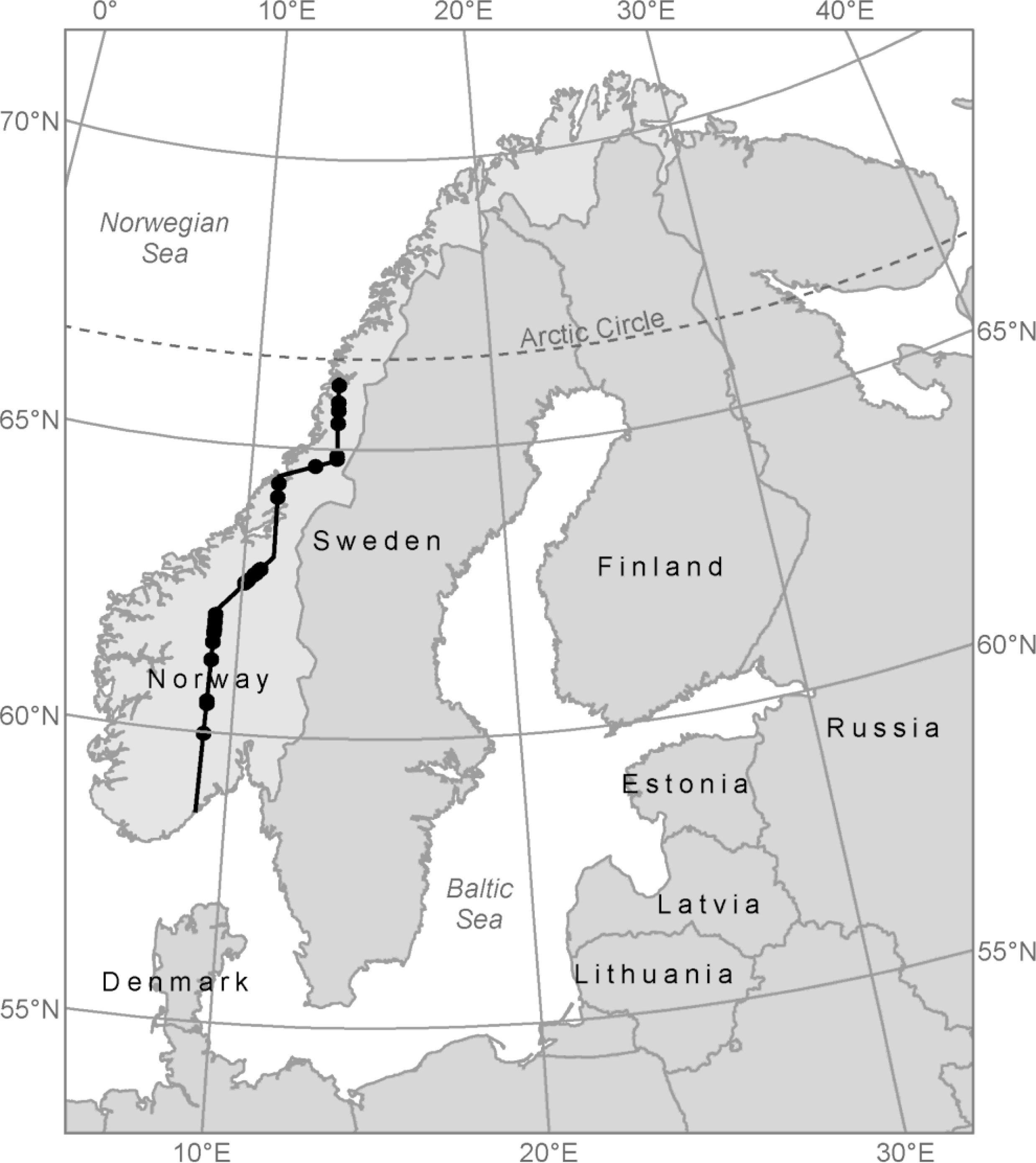
The study area covered a 1000 km long and approximately 180 m wide longitudinal transect encompassing hundreds of mountain forest and alpine elevation gradients. The transect stretches from Mo i Rana in northern Norway (66°19′N 14°9′E) to Tvedestrand in the southern part of the country (58°3′N 9°0′E) (Figure 1). Sample plots were established in the forest-tundra ecotone, which is the transition between the mountain forest and the alpine zone. In most of the localities along the transect, the terrain was characterized by rounded forms with occurrences of hummocks, rocks and boulders, but also some steep slopes. The prevalent tree species were Norway spruce (Picea abies (L.) Karst.), Scots pine (Pinus sylvestris L.), and mountain birch (Betula pubescens ssp czerepanovii).
2.2. Field Data
The field work in the transect was carried out at 25 different field sites allocated along the transect during summer 2008 in order to provide in situ tree data for analysis.
Each field site consists of two to four sample plots to cover the width of the forest-tundra ecotone. Because the width of the forest-tundra ecotone varies between different locations, the number of sample plots in each site was determined in field based on both visual and practical judgment of the altitudinal range of the ecotone in each case. Furthermore, sample plots within field sites were laid out with 50 m interdistance to avoid overlap. These procedures resulted in a total number of 77 sample plots. Two Topcon Legacy E+ 20-channel dual-frequency receivers observing pseudo range and carrier phase of both Global Positioning System and Global Navigation Satellite System satellites were used as base and rover receivers for real-time kinematic differential Global Navigation Satellite Systems (dGNSS) navigation and positioning. For each field site, the closest suitable reference point of the Norwegian Mapping Authority was selected to establish the base station. For the selection of the sample trees in the field, a modified version of the point-centerd quarter sampling method (PCQ) [19,20] was used with a maximum search distance of 25 m. This sampling method involves the division of a sample plot into four quadrants defined by the cardinal directions from the center of the sample plot. In each quadrant, the tree that was closest to the plot center in a specific tree height class was sampled independent of tree species. The tree height classes were defined as: (1) less than 1 m; (2) between 1 m and 2 m; and (3) taller than 2 m. Thus, a maximum of 12 trees could potentially be sampled in each plot. The cardinal directions were defined by using a Suunto compass, and both the closest tree and the maximum search limit were determined by using a surveyor’s tape measure in cases of doubt.
For each sample tree, several tree metrics were recorded individually. Tree species was determined and tree height was measured using a steel tape measure for smaller trees and a Vertex III hypsometer for tall trees. Stem diameter was callipered at root collar and crown diameters were measured in the cardinal directions with a steel tape measure. Finally, the precise position for each tree was determined using the dGNSS-based procedure described above.
In this study, a total of 524 trees were used, i.e., 404 mountain birch, 67 Norway spruce and 53 Scots pine. Tree heights ranged from 0.04 m to 7.80 m, and crown areas, computed as the ellipse defined by the crown diameters as the major and minor axes, from 0.001 m2 to 19.54 m2. A summary of the tree metrics is given in Table 1.
2.3. Laser Data
Airborne laser scanner data were acquired on 23 and 24 July 2006 with an Optech ALTM 3100C laser scanning system.
A Piper PA-31 Navajo aircraft carried the laser scanning system at an average flying altitude of 800 m above ground level. The flight speed was approximately 75 ms−1. The scan frequency was 70 Hz, the maximum half angle was 7°, and the average footprint diameter was estimated to 20 cm. Furthermore, the pulse repetition frequency was 100 kHz and resulted in a mean pulse density of 6.8 m−2. The 1000 km long transect was split into 98 individual flight lines to keep the flying altitude across the mountains and hence the pulse density as constant as possible.
Pre-processing of the laser scanning data was conducted by the contractor (Blom Geomatics, Norway). For all laser points, planimetric coordinates (x and y) and ellipsoidal height values were computed.
For the derivation of the terrain model, laser echoes labelled as “last-of-many” and “single” (LAST) were used. Ground echoes were classified from the planimetric coordinates and the corresponding height values of the LAST echoes, and based on an iteration distance of 1.0 m and an iteration angle of 9°, a triangulated irregular network (TIN) was derived using the TerraScan software [21]. Moreover, a digital elevation model (DEM) was computed [22] using the LAST echoes classified as ground returns to compute the terrain-related variable slope [23]. Because of the small-sized objects in question, the DEM was derived with a cell size of 0.25 m.
Laser echoes labelled as “first-of-many” and “single” (FIRST) were used for the analyses. For this purpose, FIRST echoes were projected onto the TIN surface to interpolate the corresponding terrain height values on these locations. Furthermore, the differences between the FIRST echo height values and the corresponding interpolated terrain heights were computed and stored. In this study, merely the FIRST echoes, hereafter referred to as laser echoes, with height values greater than zero were included because this criterion represents the sole indicator for the presence of objects on the terrain surface.
The ALTM 3100C instrument may record up to four echoes per laser pulse with a minimum vertical distance of 2.1 m between two subsequent echoes of an individual pulse. However, this instrument property in combination with low vegetation in the present study resulted in very few pulses with more than a single echo. Hence, the LAST and FIRST datasets were almost identical for most of the sample plots.
2.4. Computations
For assessing the capability of discriminators represented by geostatistical and standard statistical measures derived from the laser echoes to improve the classification of tree and nontree echoes, a sequence of computations had to be conducted prior to the analysis.
First, the field-measured crown diameters were used to compute elliptical tree crown polygons to select the tree echoes. Trees with a crown diameter value less than 1.0 m in at least one cardinal direction were assigned a tree crown polygon with a constant radius of 0.5 m. This was done to take into account the precision of the laser echoes (see Section 5).
Furthermore, areas within the sample plots where it was ensured that there were no trees because of the basic properties of the PCQ sampling method were identified in order to find and select nontree laser echoes. These areas were those sectors of the four quadrants that were closer to the plot center than the closest recorded tree irrespective of tree size class. In this process, the crown polygon of the closest tree was erased from the nontree sector to ensure that only laser echoes emerging from nontree objects were included.
The laser height and intensity values from the laser echoes were used for the computation of discriminators for the classification analyses. Concerning the laser height, the numerical height values were used directly. For laser intensity, the raw intensity values (IRaw) had to be normalised for the range R according to the following formula suggested by Korpela et al. [24]:
For the computation of the geostatistical and statistical measures, each of the 77 sample plots was overlaid with equally spaced grid points with an interdistance of 1 m. A moving window consisting of a circular buffer with a radius of 3 m was employed to select laser echoes for the estimation of the different geostatistical and statistical measures at each grid point both based on the laser height and intensity values. A radius of 3 m was chosen so that the moving window would be larger than the largest tree crown in the data material. Thereafter, each laser echo was assigned the computed measures of its closest grid point (Figure 2).
Semivariograms were employed as the geostatistical discriminator and were used in the analysis as a mean to characterize differences in the behavior of spatial correlation of laser height and intensity values for those tree and nontree echoes with positive height values.
A measure for the spatial correlation of a variable is derived from the calculation of the semivariances of multiple pairs of observations as a function of their separation distance [25] and is referred to as an experimental variogram. The separation distances used for estimation are represented by various distance classes which are referred to as lags. The semivariances of a dataset are computed as
The semivariances and hence the spatial variability of a variable can be illustrated by a semivariogram, which is usually referred to as a variogram. In case of spatial dependence, a univariate experimental variogram is characterized by an increase in semivariance with distance h which may level off at the so called sill or increase ad infinitum. In this study, the mean value of the semivariances of an experimental variogram was used in the analyses. This mean value was denoted SV (Table 2).
For computation of the experimental variograms specifically, variograms were calculated individually for each grid point of the 77 sample plots using the gstat spatial package [26] in the statistical computing software R [27]. The distance classes used for computation were defined to reflect the fact that lags closer to zero are expected to provide more information than lags further away. These lags were used: 0 m, 0.25 m, 0.5 m, 0.75 m, 1 m, 1.5 m, 2 m, 2.5 m, and 3 m. Furthermore, second-order stationarity was assumed which implies a constant mean, variance and covariances depending on separation only [28]. Isotropy was assumed for the spatial distributions of the laser height and intensity.
In addition to the geostatistical discriminator, statistical summary measures were employed. The arithmetic mean (AM) as the sum of values of a set of observations divided by the number of observations, the standard deviation (SD) as the square root of the averaged squares of the observations’ deviations from their mean, and the coefficient of variation (CV) as the ratio between the arithmetic mean and the standard deviation were derived both from laser height and intensity values respectively (Table 2).
2.5. Analysis
Generalised linear models (GLM) and support vector machines (SVM) were employed as classification methods in the analyses. Simple models (Table 3) from a study conducted by Stumberg et al. [18] were extended with the geostatistical and statistical measures to evaluate their potential for an improved classification performance. The two simple models included the laser height and intensity values for the GLM and the additional terrain variable slope for the SVM. A summary of the different discriminating geostatistical and statistical variables is given in Table 4.
Geostatistical and statistical measures that revealed a significant improvement of the model compared to the simple model when used individually were subsequently combined in extended models using all possible combinations (Table 3) to assess a potential contribution of these combinations for the discrimination between tree and nontree echoes.
2.5.1. GLM
GLM are commonly used in regression analysis, however, GLM also represent a suitable tool for binary classification problems predicting probabilities on a transformed scale [29]. GLM are defined by three elements consisting of the random component identifying the response variable y and its probability distribution, the link function connecting the random component to the systematic component that is again specifying the independent variables x [29,30]. In the present study, a logit link function was employed to relate the different combinations of the independent variables x to the binary response variable y (tree/nontree). Thus, the following model was fitted:
In the statistical computing software R, the different GLM models (Table 3) were fitted using the glm function of the stats package [27]. In the next step, the probabilities of the laser echoes for being a nontree echo were predicted from the fitted models. Finally, different thresholds (from p = 0.05 to p = 0.95 in 0.05 steps) for these probabilities were employed to classify the laser echoes into tree and nontree echoes for each model. For each threshold used during classification, the Cohen’s kappa coefficient [31] was estimated to identify the classification with the highest kappa coefficient.
2.5.2. SVM
SVM, which were developed by Cortes and Vapnik [32], are a suitable tool for classification, regression, and novelty detection [33,34]. By solving a quadratic optimization problem using a training set, SVM determine the hyperplane with the maximal margin of separation between two classes. In the process, the relevant information used during classification is comprised by the support vectors representing points located on the margin boundaries. Points located on the opposite side of the margin indicate overlapping classes and are reduced in influence by weighting. The error term is controlled by a so called cost or penalty parameter C and a kernel function allowing for a nonlinear separator defines the hyperplane. In the present study, the C-support vector classification was used with the radial basis function as the kernel, where γ represents a parameter regulating the radial basis function.
The different models (Table 3) were fitted with the svm function of the e1071 package [35] and a prediction of the laser echoes being a tree or nontree echo was performed for each. Using the tune.svm function of the e1071 package [33,35], the best hyperparameters C and γ were determined prior to classification and outside the leave-one-out cross-validation procedure.
2.6. Accuracy Assessment and Classification Performance
A leave-one-out cross-validation was used to assess the classification performance of the modeling with GLM and SVM. In the validation, each entire field site (i.e., several individual plots) was treated as either being part of the training dataset or the validation dataset. Thus, in each sequence of the cross-validation, models were fit with data from all sites apart from one of the sites, and the fitted models were used for classification on the single site that was excluded from the model fitting.
For each model fitted for prediction irrespective of the classification method, the total percentage of correct prediction and the Cohen’s kappa coefficient [31] were estimated to assess the classification performances. In the comparison between the simple models, i.e., HI for the GLM and HIS for the SVM (Table 3), and the respective extended models, the difference between two independent kappa coefficients was estimated using a statistics suggested by Cohen [31] that evaluates the normal curve deviate to assess the significance of such a difference:
3. Results
Classifications of the laser echoes into tree and nontree echoes using GLM and SVM models including geostatistical and statistical measures revealed total accuracies of at least 93.6% (Table 5) and 94.7% (Table 6), respectively.
Furthermore, kappa coefficients were improved by at least 0.032 (Table 5) and 0.034 (Table 4) using GLM and SVM, respectively, compared to the results of the precedent classification study conducted by Stumberg et al. [18].
3.1. GLM
The classifications of the laser echoes using GLM revealed total accuracies between 93.6% and 94.9% (Table 5). The corresponding kappa coefficients ranged from 0.526 to 0.606 indicating moderate fits for all the estimated models (Table 5).
The total accuracies differed with 1.3 percentage points between models (Table 5). Models including geostatistical or statistical measures derived from the laser intensity values (HI_ISV, HI_IAM, HI_ISD, and HI_ICV) had slightly higher accuracies, of which the models including the standard deviation or the coefficient of variation (HI_ISD and HI_ICV) had the highest accuracies of 94.9%.
Assessing the corresponding kappa coefficients, higher kappa coefficients were found for models including the geostatistical measure and/or the statistical measures represented by the arithmetic mean and the standard deviation derived from the laser height values (HI_HSV, HI_HAM, HI_HSD, and HI_HSV_HAM). The two models including the arithmetic mean, (HI_HAM) and the mean semivariance and the arithmetic mean (HI_HSV_HAM), respectively, revealed the highest kappa coefficient of 0.606 (Table 5).
Comparing the kappa coefficients of the nine estimated models to the simple model (HI) that revealed the best classification performance using GLM in the study conducted by Stumberg et al. [18], no significant contribution was found for the geostatistical and statistical measures derived from the laser intensity values (Table 5). All kappa coefficients indicated equivalent classification performances for these models, however, neither suggesting significantly worse performances.
Using the geostatistical and statistical measures derived from the laser height values, a significant contribution could be found for the mean semivariance and the arithmetic mean (Table 5). All three models including these two discriminators individually or in combination (HI_HSV, HI_HAM, and HI_HSV_HAM) revealed significantly improved classification performances compared to the simple model HI. Furthermore, the inclusion of the standard deviation or the coefficient of variation, respectively, showed a similar or significantly worse classification performance than the simple model HI (Table 5).
3.2. SVM
For the SVM classification method, the twelve different models revealed total accuracies ranging from 94.7% to 95.7% (Table 6). Furthermore, the kappa coefficients ranged between 0.576 and 0.666, indicating moderate fits for four models and substantial fits for eight models, respectively (Table 6).
The twelve models had a maximum difference in total accuracy of 1.0 percentage points (Table 6), where most models consisting of geostatistical or statistical measures derived from the laser height values (HIS_HSV, HIS_HAM, HIS_HSD, HIS_HSV_HAM, HIS_HSV_HSD, and HIS_HAM_HSD) revealed slightly higher accuracies. The highest accuracy of 95.7% was found for models including the mean semivariance and/or the standard deviation (HIS_HSV, HIS_HSD, and HIS_HSV_HSD).
Furthermore, the corresponding kappa coefficients were higher for models including the mean semivariance, the arithmetic mean, and the standard deviation derived from the laser height values, both individually and in combination with one another (HIS_HSV, HIS_HAM, HIS_HSD, HIS_HSV_HAM, HIS_HSV_HSD, and HIS_HAM_HSD). The highest kappa coefficient of 0.666 was found for the model only including the mean semivariance, indicating a substantial fit (Table 6).
The comparison between the kappa coefficients of the simple model HIS revealing the best classification performance in the study carried out by Stumberg et al. [18] and the twelve different models was used to assess the capability of the different geostatistical and statistical measures to improve previous classification.
No significant contribution could be found for any of the models consisting of the geostatistical and statistical measures derived from the laser intensity values (Table 6). The kappa coefficients for the models consisting of the mean semivariance, the standard deviation or the coefficient of variation (HIS_ISV, HIS_ISD, and HIS_ICV) indicated equivalent classification performances for the models. However, the kappa coefficient of the model including the arithmetic mean (HIS_IAM) suggested a significantly worse performance compared to the simple model HIS.
For the laser height derived geostatistical and statistical measure, a significant contribution was found for six models including the mean semivariance, the arithmetic mean, and the standard deviation individually or in combination with one another (Table 6). All these models (HIS_HSV, HIS_HAM, HIS_HSD, HIS_HSV_HAM, HIS_HSV_HSD, and HIS_HAM_HSD) had kappa coefficients of at least 0.634 improving the simple model HIS by at least 0.034 and ameliorating the moderate fit into a substantial fit. Merely the two models including the coefficient of variation or the combination of the mean semivariance, the arithmetic mean, and the standard deviation revealed no significant contribution to the basic model HIS, however, neither indicating a significantly worse classification performance. Furthermore, the mean semivariance represented the discriminator with the highest significant contribution to the basic model HIS.
4. Discussion
The classification into tree and nontree echoes including geostatistical and statistical measures revealed total accuracies that are equivalent to the results obtained by Stumberg et al. [18] for both GLM and SVM. Furthermore, the accuracies of the GLM and SVM classifications are in accordance with other studies on the discrimination of small individual trees in an environment as the forest-tundra ecotone. On an individual tree basis, these studies reported success rates of at least 90% for trees exceeding a height of 1 m [9,11,12]. These rates are comparable to the results of the present study even though individual laser echoes were used in this case.
Kappa coefficients indicated a significant improvement when including geostatistical and statistical measures for some models in comparison to the classification performances reported by Stumberg et al. [18] both using GLM and SVM. However, geostatistical and statistical measures derived from laser intensity values revealed no significant contribution to any GLM or SVM model and actually a significantly worse performance for the SVM model including the arithmetic mean was obtained. By investigating the respective distributions of values of the different measures for tree and nontree echoes (Table 4), these results seem reasonable. Particularly the summary values of the arithmetic mean and the coefficient of variation based on laser intensity values do not differ considerably, suggesting a relatively similar behavior for both tree and nontree echoes or even indicating an unprofitable effect of this discriminator on the classification performance. Also, for the laser height derived standard deviation and coefficient of variation, similar distributions of values of the different measures were found for tree and nontree echoes, thus suggesting almost no discriminating effect for the coefficient of variation in particular (Table 4). These findings are reflected in the similar or significantly worse classification performances of both GLM and SVM models including these discriminators. However, regarding the standard deviation in context with SVM, this measure reveals a significant contribution individually or in combination with the mean semivariance or the arithmetic mean indicating a positive effect of a nonlinear classification method on this specific measure. The values distributions for the arithmetic mean and the mean semivariance (Table 4) show obvious differences for tree and nontree echoes. This behavior supports the significant improvement of the simple models extended with these discriminators individually or in combination with each other for both classification methods. Furthermore, the superior performance of the geostatistical measure represented by the mean semivariance for both the GLM and SVM classification methods is in line with results obtained by Thieme et al. [15]. They found experimental variograms helpful to characterize and distinguish between tree and nontree object in a forest-tundra ecotone environment. Also Jakomulska and Clarke [17] reported a beneficial contribution of variogram-based measures for the classification of vegetation classes including grassland, rocks and woodland, however, based on optical airborne imagery. Other geostatistical features or features related to variation and structure of the laser echoes could further improve the classification. This was however not considered in the present study, but could be subject to further investigations.
In the present study the time difference between the acquisition of the ALS data and the field registrations will most likely have caused small differences between the two datasets. This would be due to tree growth and mortality or other external factors affecting the trees. We do however expect the errors introduced by this to be small.
5. Uncertainties, Errors and Accuracies
The ALTM 3100C instrument used to acquire the ALS data in the present study has an expected precision of around 0.1 m vertically and 0.2–0.3 m horizontally [37]. The expected accuracy of the geo-referenced center points at the field plots was 3–4 cm. This is derived from the expected accuracy of the reference points of 3 cm and the expected horizontal accuracy of the field recordings relative to the base station of about 2 cm. Errors and accuracies of the field measurements were not assessed in the present study, but we expect them to be small. The way the tree and nontree echoes were selected in the present study could cause some uncertainties related to the significant contribution of the mean semivariance (i.e., the height variation among the neighboring echoes). The observed effect could partly be attributed to the fact that the nontree echoes—due to the sampling procedure—could only be reliably selected from areas with presumably less echo height variation than in the areas from which the tree echoes where selected. This could have affected the analysis, but the impact of this is unknown.
6. Conclusions
To conclude, the classification of tree and nontree echoes based on previous models from the study conducted by Stumberg et al. [18] that were extended with geostatistical and statistical measures using both GLM and SVM revealed a significant contribution of the majority of the laser height-derived measures, with detection accuracies of >94% for the GLM models, and >95% for the SVM models.
Adding a geostatistical measure represented by the mean semivariance derived from the laser height values significantly improved the results compared to the basic model of both the GLM and the SVM classification methods, respectively. For this discriminator, total accuracies of at least 94% could be obtained irrespective of the classification method or being used individually or in combination with other statistical measures. The mean semivariance estimated from the laser intensity values, however, did not reveal a significant contribution to the classification performances.
With regard to the statistical measures, the arithmetic mean derived from the laser height had a significantly positive effect on the classification performances for both classification methods when being used individually and in most combinations with other measures. The laser intensity-derived arithmetic mean, however, revealed an equivalent performance for GLM and a worse performance using SVM. Concerning the standard deviation, no significant contribution could be found using GLM for neither the laser height nor intensity-derived values. Employing SVM, a significant improvement was merely obtained for the discriminator derived from the laser height. The coefficient of variation revealed no significant contribution to neither of the basic models HI and HIS. With regard to the laser height-derived coefficient of variation used in GLM, the classification performance was worse than the basic model HI.
In general, the highest improvement of a basic model was found for the HIS model using SVM extended by the mean semivariance. This result in combination with the supporting outcome of the GLM classification suggests a high potential of the mean semivariance as a geostatistical discriminator for tree and nontree echoes. However, further investigation into the characteristics of the geostatistical measure as well as its capability is needed for being able to fully understand and utilize the power of this discriminator.
Acknowledgments
This research has been funded by the Research Council of Norway (project #184636/S30). We wish to thank Blom Geomatics AS, Norway, for collection and processing of the airborne laser scanner data. Thanks also appertain to Vegard Lien at the Norwegian University of Life Sciences, who was responsible for the fieldwork. Furthermore, Nadja Stumberg would like to thank Hans Ole Ørka and Liviu Ene at the Norwegian University of Life Sciences for valuable remarks during the analysis process. Finally, we would like to thank the three anonymous reviewers for valuable and constructive comments and suggestions.
Author Contributions
Nadja Stumberg has been the main author of the manuscript, carried out calculations and analysis in the study, and conducted parts of the field work. Marius Hauglin has co-authored and revised the manuscript. Ole Martin Bollandsås has planned and prepared the field data and revised parts of the manuscript. Terje Gobakken has prepared the remote sensing data, supervised parts of the study and has revised parts of the manuscript. Erik Næsset has planned and prepared the remote sensing data, detailed the field sampling design, supervised the study and revised parts of the manuscript.
Conflicts of Interest
The authors declare no conflict of interest.
References
- Kirschbaum, M.; Fischlin, A. Climate Change Impacts on Forests. In Climate Change 1995: Impacts, Adaptations and Mitigation of Climate Change: Scientific-Technical Analysis. Contribution of Working Group II to the Second Assessment Report of the Intergovernmental Panel on Climate Change; Watson, R., Zinyowerea, M.C., Moss, R.H., Eds.; Cambridge University Press: Cambridge, UK, 1996; pp. 99–129. [Google Scholar]
- Harper, K.A.; Danby, R.K.; de Fields, D.L.; Lewis, K.P.; Trant, A.J.; Starzomski, B.M.; Savidge, R.; Hermanutz, L. Tree spatial pattern within the forest–tundra ecotone: A comparison of sites across Canada. Can. J. For. Res 2011, 41, 479–489. [Google Scholar]
- Arctic Climate Impact Assessment (ACIA). Impacts of a Warming Arctic: Arctic Climate Impact Assessment; Cambridge University Press: Cambridge, UK, 2004. [Google Scholar]
- Callaghan, T.V.; Werkman, B.R.; Crawford, R.M.M. The tundra-taiga interface and its dynamics: Concepts and applications. Ambio 2002, 12, 6–14. [Google Scholar]
- Holtmeier, F.-K.; Broll, G. Sensitivity and response of northern hemisphere altitudinal and polar treelines to environmental change at landscape and local scales. Glob. Ecol 2005, 14, 395–410. [Google Scholar]
- Hyyppa, J.; Kelle, O.; Lehikoinen, M.; Inkinen, M. A segmentation-based method to retrieve stem volume estimates from 3-D tree height models produced by laser scanners. IEEE Trans. Geosci. Remote Sens 2001, 39, 969–975. [Google Scholar]
- Persson, A.; Holmgren, J.; Soderman, U. Detecting and measuring individual trees using an airborne laser scanner. Photogramm. Eng. Remote Sens 2002, 68, 925–932. [Google Scholar]
- Solberg, S.; Nasset, E.; Bollandsas, O.M. Single tree segmentation using airborne laser scanner data in a structurally heterogeneous spruce forest. Photogramm. Eng. Remote Sens 2006, 72, 1369–1378. [Google Scholar]
- Nasset, E.; Nelson, R. Using airborne laser scanning to monitor tree migration in the boreal–alpine transition zone. Remote Sens. Environ 2007, 110, 357–369. [Google Scholar]
- Rees, W.G. Characterisation of Arctic treelines by LiDAR and multispectral imagery. Polar Rec 2007, 43, 345–352. [Google Scholar]
- Thieme, N.; Martin Bollandsas, O.; Gobakken, T.; Nasset, E. Detection of small single trees in the forest–tundra ecotone using height values from airborne laser scanning. Can. J. Remote Sens 2011, 37, 264–274. [Google Scholar]
- Nasset, E. Influence of terrain model smoothing and flight and sensor configurations on detection of small pioneer trees in the boreal–alpine transition zone utilizing height metrics derived from airborne scanning lasers. Remote Sens. Environ 2009, 113, 2210–2223. [Google Scholar]
- Rossi, R.E.; Mulla, D.J.; Journel, A.G.; Franz, E.H. Geostatistical tools for modeling and interpreting ecological spatial dependence. Ecol. Monogr 1992, 62, 277–314. [Google Scholar]
- Fry, D.L.; Stephens, S.L. Stand-level spatial dependence in an old-growth Jeffrey pine–mixed conifer forest, Sierra San Pedro Martir, Mexico. Can. J. For. Res 2010, 40, 1803–1814. [Google Scholar]
- Thieme, N.; Bollandsas, O.M.; Gobakken, T.; Nasset, E. Assessing Spatial Variation for Tree and Non-Tree Objects in a Forest-Tundra Ecotone in Airborne Laser Scanning Data. Proceedings of the SilviLaser 2011: 11th International Conference on LiDAR Applications for Assessing Forest Ecosystems, Hobart, Australia, 16–20 October 2011; pp. 325–332. Available online: http://www.iufro.org (accessed on 1 February 2012).
- Wulder, M.A.; LeDrew, E.F.; Franklin, S.E.; Lavigne, M.B. Aerial image texture information in the estimation of northern deciduous and mixed wood forest Leaf Area Index (LAI). Remote Sens. Environ 1998, 64, 64–76. [Google Scholar]
- Jakomulska, A.; Clarke, K.C. Variogram-Derived Measured of Textural Image Classification: Application to Large-Scale Vegetation Mapping. In In geoENV III—Geostatistics for Environmental Applications; Monestiez, P., Allard, D., Froidevaux, R., Eds.; Kluwer Academic Publishers: Dordrecht, The Netherlands, 2001; pp. 345–355. [Google Scholar]
- Stumberg, N.; Orka, H.O.; Bollandsas, O.M.; Gobakken, T.; Nasset, E. Classifying tree and nontree echoes from airborne laser scanning in the forest–tundra ecotone. Can. J. Remote Sens 2012, 38, 655–666. [Google Scholar]
- Cottam, G.; Curtis, J.T. The use of distance measures in phytosociological sampling. Ecology 1956, 37, 451–460. [Google Scholar]
- Warde, W.; Petranka, J.W. A correction factor table for missing point-center quarter data. Ecology 1981, 62, 491–494. [Google Scholar]
- Terrasolid. TerraScan User’s Guide. Available online: http://www.terrasolid.fi (accessed on 26 September 2011).
- QCoherent Software. Getting Started with LP360. Available online: http://www.qcoherent.com (accessed on 8 February 2012).
- Burrough, P.A.; McDonnell, R.; Burrough, P.A. Principles of Geographical Information Systems; Oxford University Press: Oxford, UK/New York, NY, USA, 1998. [Google Scholar]
- Korpela, I.; Orka, H.O.; Maltamo, M.; Tokola, T.; Hyyppa, J. Tree species classification using airborne LiDAR—Effects of stand and tree parameters, downsizing of training set, intensity normalization, and sensor type. Silva Fenn 2010, 44, 319–339. [Google Scholar]
- Isaaks, E.H.; Srivastava, R.M. An Introduction to Applied Geostatistics; Oxford University Press: Oxford, UK, 1989. [Google Scholar]
- Pebesma, E.J. Multivariable geostatistics in S: The gstat package. Comput. Geosci 2004, 30, 683–691. [Google Scholar]
- The R Development Core Team. R: A Language and Environment for Statistical Computing; The R Development Core Team: Vienna, Austria, 2011; Available online: http://www.lsw.uni-heidelberg.de/users/christlieb/teaching/UKStaSS10/R-refman.pdf (accessed on 31 May 2010). [Google Scholar]
- Webster, R.; Oliver, M.A. Geostatistics for Environmental Scientists; Wiley: Chichester, UK, 2001. [Google Scholar]
- Dalgaard, P. Introductory Statistics with R; Springer: New York, NY, USA, 2008. [Google Scholar]
- Agresti, A. An Introduction to Categorical Data Analysis; Wiley: Hoboken, NJ, USA, 2007. [Google Scholar]
- Cohen, J. A coefficient of agreement for nominal scales. Educ. Psychol. Meas 1960, 20, 37–46. [Google Scholar]
- Cortes, C.; Vapnik, V. Support-vector networks. Mach. Learn 1995, 20, 273–297. [Google Scholar]
- Karatzoglou, A.; Meyer, D.; Hornik, K. Support Vector Machines in R. J. Stat. Softw 2006, 15, 1–28. [Google Scholar]
- Meyer, D. Support Vector Machines: The Interface to Libsvm in Package e1071. Available online: http://cran.r-project.org/web/packages/e1071/ (accessed on 26 September 2011).
- Dimitriadou, E.; Hornik, K.; Leisch, F.; Meyer, D.; Weingessel, A. e1071: Misc Functions of the Department of Statistics (e1071). Available online: http://cran.r-project.org/web/packages/e1071/ (accessed on 26 September 2011).
- Landis, J.R.; Koch, G.G. The measurement of observer agreement for categorical data. Biometrics 1977, 33, 159–174. [Google Scholar]
- Lane, T. An Assessment of Vertical Accuracy of Optech’s ALTM 3100 Airborne Laser Scanning System. Proceedings of the ISPRS WGI/2 Workshop, Banff, AB, Canada, 7–10 June 2005.


| Tree Species | Characteristics | n | Mean | Min. | Max. |
|---|---|---|---|---|---|
| Mountain birch | Height (m) | 404 | 1.41 | 0.04 | 7.80 |
| Diameter (cm) | 404 | 4.24 | 0.10 | 34.00 | |
| Crown area (m2) | 404 | 1.13 | 0.001 | 19.54 | |
| Norway spruce | Height (m) | 67 | 1.67 | 0.07 | 7.00 |
| Diameter (cm) | 65 a | 6.54 | 0.20 | 19.10 | |
| Crown area (m2) | 67 | 1.45 | 0.006 | 5.69 | |
| Scots pine | Height (m) | 53 | 1.33 | 0.10 | 5.10 |
| Diameter (cm) | 53 | 5.00 | 0.30 | 18.90 | |
| Crown area (m2) | 53 | 0.81 | 0.002 | 7.28 | |
Note:aMissing values due to tree properties.
| Based on | Discriminator | Abbreviation |
|---|---|---|
| Laser Height | Mean Semivariance | HSV |
| Arithmetic Mean | HAM | |
| Standard Deviation | HSD | |
| Coefficient of Variation | HCV | |
| Laser Intensity | Mean Semivariance | ISV |
| Arithmetic Mean | IAM | |
| Standard Deviation | ISD | |
| Coefficient of Variation | ICV | |
| Classification | Models a |
|---|---|
| Basic models GLM | HI_HSV, HI_HAM, HI_HSD, HI_HCV, HI_ISV, HI_IAM, HI_ISD, HI_ICV |
| Additional models GLM | HI_HSV_HAM |
| Basic models SVM | HIS_HSV, HIS_HAM, HIS_HSD, HIS_HCV, HIS_ISV, HIS_IAM, HIS_ISD, HIS_ICV |
| Additional models SVM | HIS_HSV_HAM, HIS_HSV_HSD, HIS_HAM_HSD, HIS_HSV_HAM_HSD |
Note:aHI and HIS indicate the simple models for GLM and SVM, respectively. For further abbreviations see Table 2.
| Class | Variable | Mean | Min. | Max. |
|---|---|---|---|---|
| Tree | Height (m) | 1.59 | 0.04 | 6.49 |
| Mean semivariance | 0.95 | 0.00 | 6.28 | |
| Mean | 1.25 | 0.08 | 4.24 | |
| Standard deviation | 0.91 | 0.00 | 2.58 | |
| Coefficient of variation | 0.80 | 0.00 | 2.24 | |
| Intensity | 51.62 | 4.24 | 90.95 | |
| Mean semivariance | 114.36 | 0.00 | 603.08 | |
| Mean | 53.80 | 34.21 | 76.58 | |
| Standard deviation | 10.86 | 0.00 | 22.80 | |
| Coefficient of variation | 0.21 | 0.00 | 0.48 | |
| Slope (°) | 16.49 | 1.05 | 49.89 | |
| Non-tree | Height (m) | 0.17 | 0.01 | 4.72 |
| Mean semivariance | 0.04 | 0.00 | 4.02 | |
| Mean | 0.19 | 0.04 | 4.17 | |
| Standard deviation | 0.12 | 0.00 | 2.46 | |
| Coefficient of variation | 0.51 | 0.00 | 2.64 | |
| Intensity | 56.22 | 0.51 | 110.82 | |
| Mean semivariance | 60.14 | 0.00 | 1462.73 | |
| Mean | 56.10 | 10.65 | 94.01 | |
| Standard deviation | 7.56 | 0.00 | 38.26 | |
| Coefficient of variation | 0.14 | 0.00 | 1.04 | |
| Slope (°) | 16.54 | 0.005 | 79.68 | |
| Model a | p | Accuracy | Kappa | Z b | |
|---|---|---|---|---|---|
| HI_HSV | 0.85 | 0.947 | 0.605 | 2.333 | * |
| HI_HAM | 0.85 | 0.946 | 0.606 | 2.482 | * |
| HI_HSD | 0.80 | 0.943 | 0.590 | 1.255 | |
| HI_HCV | 0.75 | 0.936 | 0.526 | 3.469 | ** |
| HI_ISV | 0.75 | 0.948 | 0.570 | 0.285 | |
| HI_IAM | 0.70 | 0.948 | 0.565 | 0.626 | |
| HI_ISD | 0.65 | 0.949 | 0.573 | 0.029 | |
| HI_ICV | 0.70 | 0.949 | 0.565 | 0.577 | |
| HI_HSV_HAM | 0.85 | 0.946 | 0.606 | 2.480 | * |
| HI | 0.75 | 0.949 | 0.573 |
Notes: Level of significance:*<0.05.**<0.005.aHI indicates the simple model. For further abbreviations see Table 2.bAs received by the comparison between two independent kappa coefficients, i.e., the simple model HI and the respective extended model.
| Model a | C b | γ c | Accuracy | Kappa | Z d | |
|---|---|---|---|---|---|---|
| HIS_HSV | 100 | 0.1 | 0.957 | 0.666 | 4.995 | ** |
| HIS_HAM | 1000 | 0.1 | 0.956 | 0.655 | 4.183 | ** |
| HIS_HSD | 100 | 0.1 | 0.957 | 0.660 | 4.539 | ** |
| HIS_HCV | 100 | 0.1 | 0.951 | 0.605 | 0.352 | |
| HIS_ISV | 1000 | 0.1 | 0.953 | 0.613 | 0.901 | |
| HIS_IAM | 1000 | 0.1 | 0.947 | 0.576 | 1.772 | ′ |
| HIS_ISD | 100 | 0.1 | 0.953 | 0.608 | 0.570 | |
| HIS_ICV | 1000 | 0.1 | 0.950 | 0.605 | 0.353 | |
| HIS_HSV_HAM | 100 | 0.1 | 0.955 | 0.643 | 3.186 | ** |
| HIS_HSV_HSD | 100 | 0.1 | 0.957 | 0.664 | 4.875 | ** |
| HIS_HAM_HSD | 100 | 0.1 | 0.954 | 0.634 | 2.556 | * |
| HIS_HSV_HAM_HSD | 1000 | 0.1 | 0.952 | 0.621 | 1.552 | |
| HIS | 1000 | 0.1 | 0.953 | 0.600 |
Notes: Level of significance: ′ <0.1.*<0.05.**<0.005.aHIS indicates the simple model. For further abbreviations see Table 2.bCost or penalty parameter.cParameter regulating the radial basis function.dAs received by the comparison between two independent kappa coefficients, i.e., the simple model HIS and the respective extended model.
© 2014 by the authors; licensee MDPI, Basel, Switzerland This article is an open access article distributed under the terms and conditions of the Creative Commons Attribution license (http://creativecommons.org/licenses/by/3.0/).
Share and Cite
Stumberg, N.; Hauglin, M.; Bollandsås, O.M.; Gobakken, T.; Næsset, E. Improving Classification of Airborne Laser Scanning Echoes in the Forest-Tundra Ecotone Using Geostatistical and Statistical Measures. Remote Sens. 2014, 6, 4582-4599. https://doi.org/10.3390/rs6054582
Stumberg N, Hauglin M, Bollandsås OM, Gobakken T, Næsset E. Improving Classification of Airborne Laser Scanning Echoes in the Forest-Tundra Ecotone Using Geostatistical and Statistical Measures. Remote Sensing. 2014; 6(5):4582-4599. https://doi.org/10.3390/rs6054582
Chicago/Turabian StyleStumberg, Nadja, Marius Hauglin, Ole Martin Bollandsås, Terje Gobakken, and Erik Næsset. 2014. "Improving Classification of Airborne Laser Scanning Echoes in the Forest-Tundra Ecotone Using Geostatistical and Statistical Measures" Remote Sensing 6, no. 5: 4582-4599. https://doi.org/10.3390/rs6054582