Improving the Geolocation Algorithm for Sensors Onboard the ISS: Effect of Drift Angle

Abstract

The drift angle caused by the Earth’s self-rotation may introduce rotational displacement artifact on the geolocation results of imagery acquired by an Earth observing sensor onboard the International Space Station (ISS). If uncorrected, it would cause a gradual degradation of positional accuracy from the center towards the edges of an image. One correction method to account for the drift angle effect was developed. The drift angle was calculated from the ISS state vectors and positional information of the ground nadir point of the imagery. Tests with images acquired by the International Space Station Agriculture Camera (ISSAC) using Google Earth^™ as a reference indicated that applying the drift angle correction can reduce the residual geolocation error for the corner points of the ISSAC images from over 1000 to less than 500 m. The improved geolocation accuracy is well within the inherent geolocation uncertainty of up to 800 m, mainly due to imprecise knowledge of the ISS attitude and state parameters required to perform the geolocation algorithm.

1. Introduction

As the largest manmade object in the outer space, the International Space Station (ISS) not only provides a laboratory for scientific experiments in a wide range of disciplines, but also offers a unique platform for Earth observation. Compared with a traditional satellite, the ISS orbits the Earth at a lower altitude (350~420 km above the sea level), a higher inclination angle (~51.6°) and a shorter period (90 min), allowing Earth observing sensors onboard it covering nearly 75% of the inhabited land surface with potentially high spatial resolution and short revisit time of approximately 3 days [1]. In addition, unlike satellite-borne sensors, payload systems onboard the ISS can be serviced or upgraded, if necessary.

With the above-mentioned merits of the ISS as an Earth observation platform, many Earth observing payload systems have been developed, such as the International Space Station Agricultural Camera (ISSAC) for precision farming [2], FOCUS for monitoring high temperature events [3], the Station High-sensitivity Ocean Research Experiment (SHORE) for mapping coral reefs, atolls, tidal areas and shore/ocean interfaces [4] and the Hyperspectral Imager for the Coastal Ocean (HICO) for monitoring coastal zone environment, the maritime atmosphere, and distribution of fires and active volcanoes [5]. The advantages of the ISS as an Earth observing platform also pose challenges in applying the observations to study the Earth. Among them, the most challenging is to precisely determine geographic locations of imagery on the Earth surface [6]. Because of its low orbit, the ISS experiences large variations in its attitude and altitude [7], making geolocation of imagery acquired by the ISS sensors much more complicated than that by satellite sensors.

To precisely geo-reference the Earth observing imagery acquired by the payload systems onboard the ISS, Dou et al. developed a quaternion-based geolocation algorithm [8]. Applying the algorithm to the images acquired by the ISSAC [2,9] and comparing the results with Google Earth^™, they estimated that the algorithm has a geolocation accuracy of 190 ± 140 m with maximum errors less than 500 m in nadir points if the orientation of the sensor in the ISS body-fixed coordinate system was accounted for. This accuracy is well within the inherent geolocation uncertainty of up to ~800 m, mainly due to imprecise knowledge of the ISS state and attitude parameters required to perform the geolocation algorithm. However, among the residual geolocation errors, a peculiar pattern emerged (shown as squares in Figure 1): the geolocated images show a small, yet statistically significant, latitude- and orbit-dependent rotational displacement. We defined the rotational displacement as the angle that an image has to rotate to arrive at the proper orientation; it is positive if the rotation is clockwise and negative for counter-clockwise rotation. Although this rotational displacement does not affect the geolocation accuracy for nadir points, it does cause a gradual degradation of geolocation accuracy towards edges of an image. To correct for this rotational displacement, Dou et al. proposed a temporary correction in the geolocation algorithm of using two mean values of squares in Figure 1, one for ascending and another for descending orbits. Specifically, the geolocated images were further rotated by −1.217° for descending orbits and by 1.787° for ascending orbits. Since this rotational displacement error is not random, and depends on the latitude and orbit directions, it is apparent that the temporary correction is not ideal, even though it does provide a certain level of correction.

The objective of this paper is to investigate the cause of this rotational error and to provide a correction to further improve the Dou et al. geolocation algorithm [8].

2. Method and Data

2.1. Geolocation Algorithm

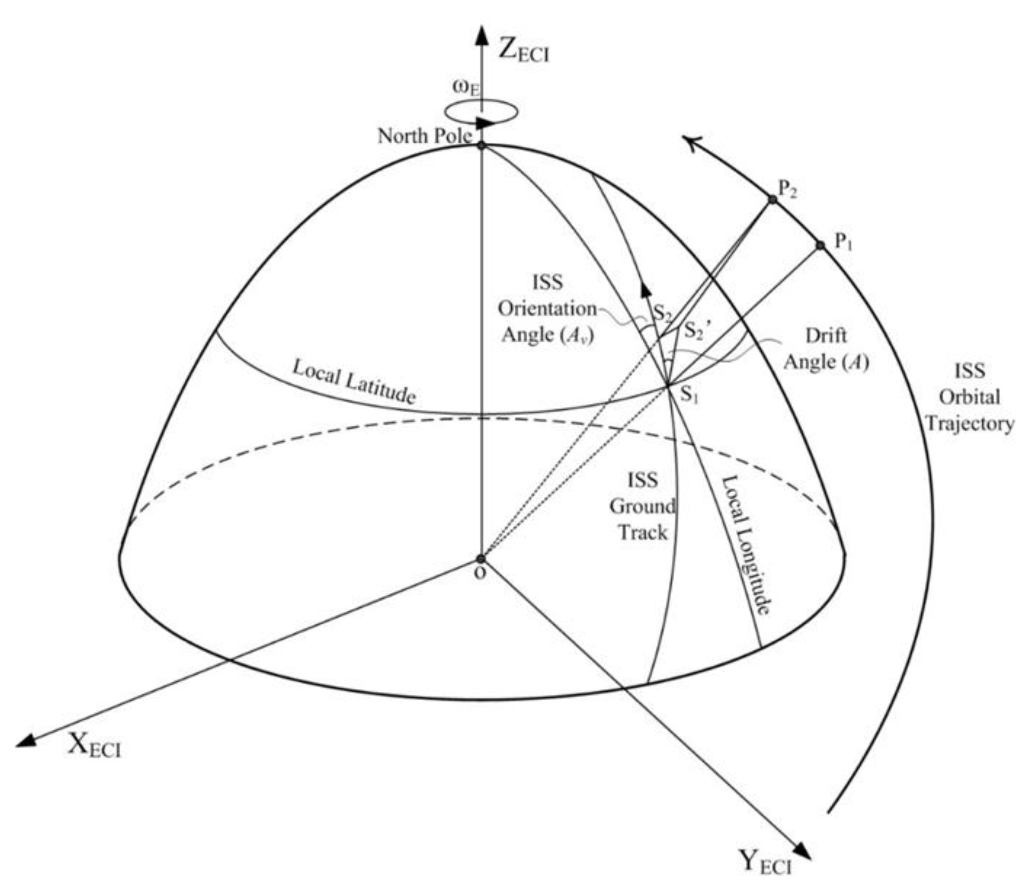
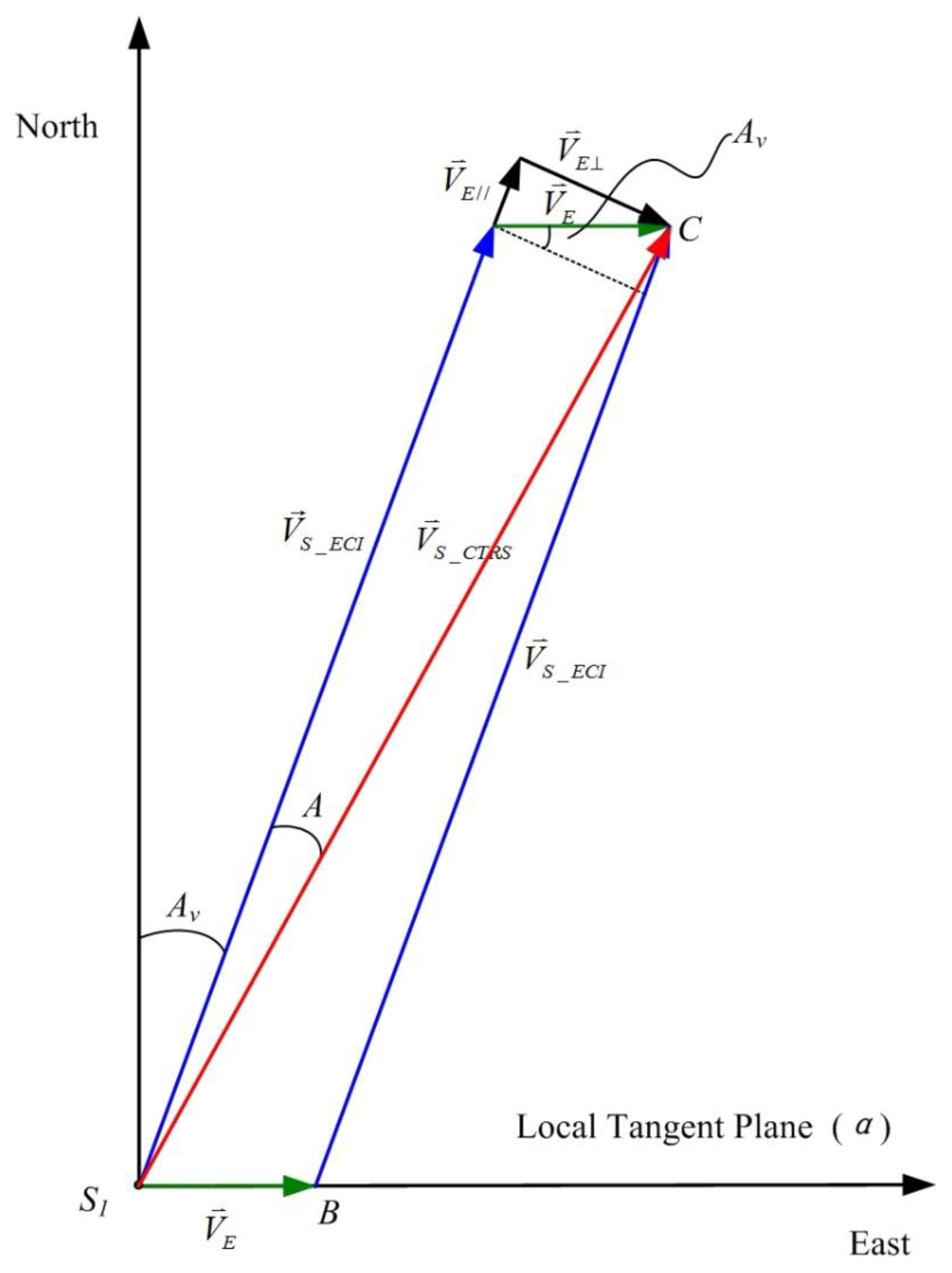
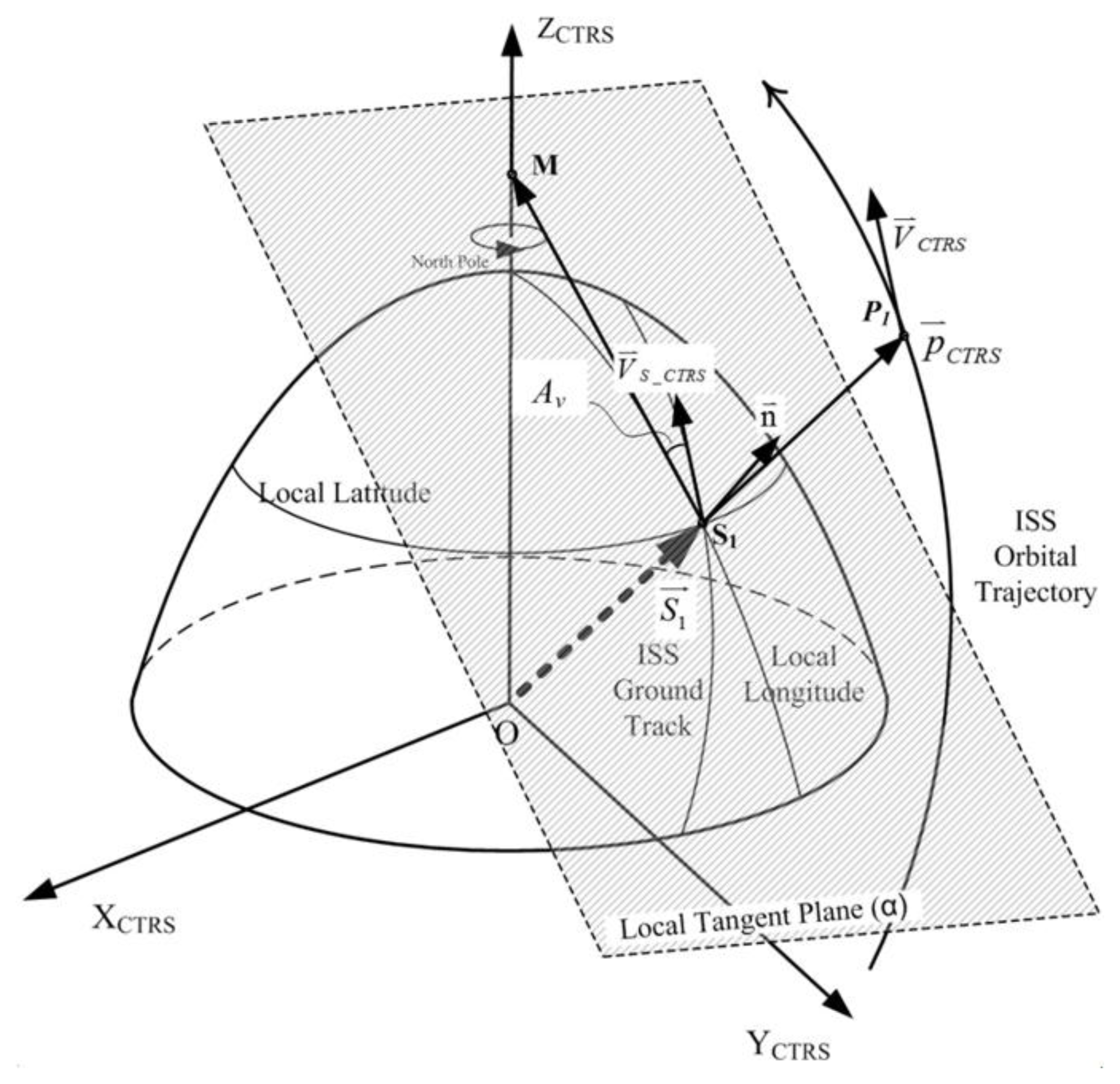
Dou et al. [8] developed a forward quaternion-based geolocation algorithm to geo-reference images acquired by the Earth observing sensors onboard the ISS. The algorithm also accounts for the tilting capability that some sensors possess; for example, the ISSAC can tilt up to 30° in both port and starboard directions of the ISS to actively seek targets [10], and HICO can tilt up to 45° [5]. Figure 2 summarizes the general procedures of the algorithm. Conceptually, geolocation starts by defining a look vector associated with a target pixel on the ground in the Sensor coordinate system, with its origin coinciding with the focus of the lens. Through a series of coordinate system transformations, the look vector is finally defined in the Conventional Terrestrial Reference System (CTRS). The CTRS is an Earth Centered Rotating (ECR) reference frame with its origin at the mass center of the Earth, its Z-axes aligning with the International Reference Pole (IRP) and X-axes with International Reference Meridian (IRM). In the CTRS reference frame, the geographic location of the pixel is sought as the intersection of the transformed look vector and the Earth surface, which is defined as an ideal Earth ellipsoid overlaid by a digital elevation model [8].

2.2. Drift Angle

Figure 3 illustrates geometric relationship of a sensor onboard the ISS and its imaging objects on the ground in an Earth Centered Inertial (ECI) coordinate system (CS), which is fixed in space and does not rotate with the Earth. At times t₁ and t₂, the ISS passes positions P₁ and P₂ in an orbit. At t₁, the sensor takes an image with its nadir pixel at point S₁ on the ground, and at t₂, the sensor takes another image. If the Earth is stationary, then the nadir pixel of the 2nd image would be at S₂ on the ground; but in reality, because of the Earth self-rotation, the nadir pixel is actually $S_2^{\prime }$. The vector $\overrightarrow{S_1{S}_2}$ defines the ground track of the ISS orbit between t₁ and t₂ and the vector $\overrightarrow{S_1{S}_2^{\prime }}$ defines the nadir target movement during the time period. The angle formed by the two vectors of $\overrightarrow{S_1{S}_2}$ and $\overrightarrow{S_1{S}_2^{\prime }}$ is the drift angle, which is positive if the imaging target drifts to the right side of the ISS flying direction (clockwise) and negative to the left side (counter-clockwise). The drift angle, if uncorrected, would cause a rotational artifact in imagery taken from the space [11]. For the ascending case shown in Figure 3, the target drifts to the right (clockwise) of the ISS ground moving direction ( $\overrightarrow{S_1{S}_2}$). Therefore, imagery has to be rotated counter-clockwise to correct this artifact. The target would move to the left for descending orbits, requiring a clockwise rotational correction. When the ISS is at its orbital apexes, the two vectors align with each other, and hence the drift angle is null. Because the linear rotational speed of the Earth decreases from the Equator to the Poles, the drift angle has its highest absolute value when the ISS crosses the Equator, decreases gradually toward zero as the ISS approaches its orbital apex points and increases again as the ISS passes the orbital apexes and moves toward the Equator. If the drift angle was not accounted for in the geolocation process, or there was not a yaw steering mechanism on the spacecraft to adjust the yaw orientation angles accordingly [12–14], a systematic rotational displacement pattern, as shown in Figure 1, would appear in the results [15]. The drift angle can be calculated from the spacecraft orbital elements, i.e., the eccentricity, semi-major axis, inclination, longitude of the ascending node, argument of periapsis and mean anomaly at epoch [11,13,15]. However, to be consistent with the Dou et al. [8] algorithm, which does not use these orbital element data, we propose a method to compute, by using the unit quaternion, the drift angle from the ISS state vectors and the positional information of the ground nadir point of the imagery. The drift angle effect also degrades the imaging quality due to the relative movement between the sensor and the target [16,17], which, however, is out of the scope of this study.

2.3. Drift Angle Calculation

The drift angle can be determined from trigonometry in the local tangent plane at point S₁ (Figure 4). Due to the Earth self-rotation, S₁ experiences a linear velocity, V⃗_E (green arrow):

$$\left|{\overrightarrow{V}}_E\right|=R^{\prime }{\omega }_E=R{\omega }_E\hspace{0.17em}\text{cos\hspace{0.17em}}\delta$$

(1)

where δ is the local latitude at S₁, R and R′ are the radii of the Earth and the local latitude circle, respectively, and ω_E is the Earth self-rotation rate. V⃗_{S_ECI} (blue arrow) would be the ISS’s projected velocity at S₁ on the ground if the Earth was not rotating. V⃗_{S_CTRS} (red arrow) is the projected velocity at S₁ on the ground accounting for the Earth rotation. Apparently, V⃗_{S_CTRS} = V⃗_{S_ECI} + V⃗_E. We further partition V⃗_E into V⃗_E// parallel to and V⃗_E⊥ perpendicular to V⃗_{S_ECI}:

$$\begin{array}{l}\left|{\overrightarrow{V}}_{E//}\right|\hspace{0.17em}=R{\omega }_E\hspace{0.17em}\text{cos\hspace{0.17em}}\delta \hspace{0.17em}\text{sin\hspace{0.17em}}{A}_v\\ \left|{\overrightarrow{V}}_{E\perp }\right|\hspace{0.17em}=R{\omega }_E\hspace{0.17em}\text{cos\hspace{0.17em}}\delta \hspace{0.17em}\text{sin\hspace{0.17em}}{A}_v\end{array}$$

(2)

Here, A_v is the spacecraft orientation angle. The drift angle, A, is:

$$A=\text{arcsin}(\frac{\left|{\overrightarrow{V}}_{E\perp }\right|}{\left|{\overrightarrow{V}}_{S\_CTRS}\right|})=\text{arcsin}(\frac{R{\omega }_E\hspace{0.17em}\text{cos}\hspace{0.17em}\delta \hspace{0.17em}\text{cos}\hspace{0.17em}{A}_v}{\left|{\overrightarrow{V}}_{S\_CTRS}\right|})$$

(3)

Figure 5 illustrates geometric details in estimating the ISS orientation angle (A_v), which is defined in the CTRS coordinate system (an ECR reference frame). The coordinates of $S_1\hspace{0.17em}(R=\left|\overrightarrow{S_1}\right|)$ as well as its geographic latitude (δ) and longitude can be estimated from Dou et al. [8] geolocation algorithm (Figure 2). The projected velocity of the ISS on the ground in the local tangent plane, V⃗_{S_CTRS}, is:

$${\stackrel{\rightharpoonup }{V}}_{S\_CTRS}=\frac{R}{r}{\overrightarrow{V}}_{CTRS}$$

(4)

where r and V⃗_CTRS are, respectively, the geocentric range distance and the velocity of the ISS, both of which can be obtained from the ISS Broadcast Ancillary Data (BAD) packages. The ISS orientation angle A_v is the angle formed by V⃗_{S_CTRS} and $\overrightarrow{S_{1}M}$, where M is the intersection point of Z_CTRS and the tangent plane (α), i.e., $A_v=\text{arcos}({\overrightarrow{V}}_{S\_CTRS}\times \overrightarrow{S_{1}M})$. If the local tangent plane is parallel with Z-axis, then $A_v=\text{arcos}([0,0,1]\times \overrightarrow{SM})$, where [0,0,1] represents Z-axis [8].

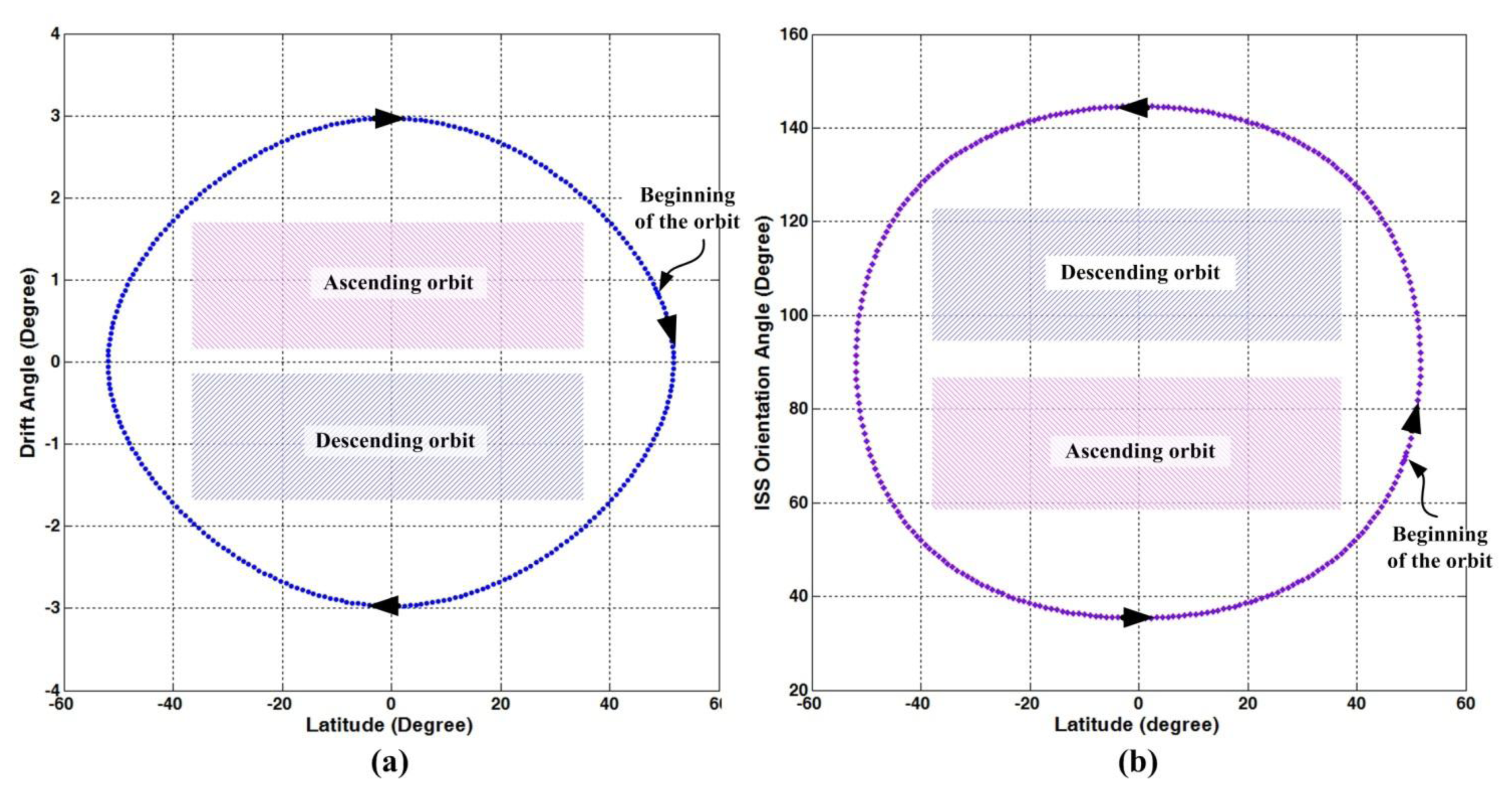
3. Results and Discussion

Figure 6a shows the changes of the drift angle determined by a sensor onboard the ISS in an ideal setting, i.e., the Sensor coordinate system aligns perfectly with the ISS body-fixed coordinate system. To estimate the drift angle, the input parameters, including position and velocity vectors and attitude quaternion of ISS, were extracted from the ISS BAD packages for a time period from 2008:320:00:00:00 (yyyy:ddd:hh:mm:ss) to 2008:320:01:31:40 (about one orbit cycle of the ISS) at an interval of 20 s. As shown, the drift angle decreases from the Equator to the orbital apexes, the sign of the angle switches after passing the apex. The drift angle reaches the maximum and minimum value of ±2.972 at the Equator in the ascending and descending orbit directions, respectively, and has 0 at the apexes, which for the ISS are at latitudes of ±51.675°. As a comparison, Figure 6b shows the variations of the orientation angles of the ISS (A_v) over the same orbit as in Figure 6a.

To assess the drift angle effect on applications, we used thirteen images (10 in ascending and 3 in descending orbits) acquired by the ISSAC over the continental US with latitude ranging from about 25°N to 50°N. The Dou et al. [8] geolocation algorithm was applied to the images and the geolocated images were compared with Google Earth^™. Two examples are shown in Figure 7, where the geolocated images clearly have a counter-clockwise (Figure 7a) and clockwise (Figure 7b) residual rotational displacement with respect to Google Earth^™ for descending and ascending orbit, respectively. The residual rotational displacement estimated for all the 13 images are plotted in Figure 1 (squares) as a function of the latitudes of the images’ centers. We then computed the actual drift angle corresponding to the center of each image; the computed drift angles are also plotted in Figure 1 (diamonds). Clearly, the residual rotational displacements and the drift angles have a very similar pattern of variations with the center latitudes of the images. We estimated that over 99% of variability in the residual rotational displacement can be explained by the drift angle. However, the two are not exactly the same; there was a systematic bias (pluses in Figure 1) that seems to be independent of the center latitudes. The biases varied between a tight range of 0.214° to 0.583° with an average of 0.339 ± 0.095.

To geolocate images acquired by a sensor, the relative position and orientation (or alignment) of the Sensor coordinate system with respect to the ISS body-fixed coordinate system need to be known (Figure 2). For ad hoc sensor payloads onboard the ISS, this piece of information can be estimated via calibration/validation procedure [18,19] using acquired images. Dou et al. [8] estimated that the ISSAC sensor coordinate system has a roll misalignment angle of about −0.45° with respect to the ISS body-fixed coordinate system, but they were unable to determine the yaw misalignment angle because the drift angle effect was not considered in the geolocation algorithm. The bias shown in Figure 1 (pluses) may reflect the yaw angle misalignment. Therefore, we hypothesized that the observed residual rotational displacement in geolocated ISSAC images (squares in Figure 1) comprises two parts: a systematic misalignment for yaw angle between the ISSAC Sensor and the ISS body-fixed coordinate system, and a latitude- and orbit-dependent drift angle effect.

To test the hypothesis, we modified the Dou et al. [8] geolocation algorithm by assuming a yaw angle misalignment of 0.339°, the mean value of “+” data in Figure 1. We then ran the geolocation algorithm to the ISSAC images, followed by rotating each of the resultant images by the drift angle determined for the corresponding center latitude of the images. Finally, we compared the rotational displacement and geographic positions of the four corners of each image. As shown in Figure 8a, before the rotational displacement correction, the rotational residual showed a latitude- and orbit-dependent pattern with the maximum of 2.6° and −1.85° for ascending and descending orbits, respectively, and after the correction, it varied around zero with a standard deviation of 0.098. Figure 8b summarizes the geolocation errors before and after applying the drift angle correction. Before the correction, the average errors of the corner points of the images was 1077 m and the maximum error of 1280 m, after the correction, the average errors was 416 m and the maximum error was 490 m, well within the maximum inherent uncertainty of up to 800 m due to precision in determining the ISS’ attitude quaternion and state vectors [8].

One of the novelties of Dou et al. [8] geolocation algorithm is transforming the payload viewing vector from the ISS orbital to ECR coordinate system directly, bypassing the intermediate steps of orbital to ECI and ECI to ECR transformations. The complex transformation from ECI to ECR would account for Earth rotation, but requires information that describes the orientation of the rotating Earth such as polar motion, sidereal time, astronomic nutation, and precession, which are not readily available in the ISS BAD packages. However, the cost associated with the direct transformation from the ISS orbital to ECR is that it introduces a rotational residual in the geolocation results. The drift angle correction method that we presented is to explicitly compensate the Earth self-rotation effect on geolocation using information that is readily available from the ISS BAD packages.

The combination of the Dou et al. [8] geolocation and the drift angle correction algorithms provides an alternative method to perform the geolocation for Earth observing imagery obtained in an Low Earth Orbit (LEO) spacecraft, such as the ISS or China Tiangong-1, which directly reports the spacecraft’s state data (position and velocity vectors) in ECR coordinate system.

4. Conclusions

The drift angle caused by the Earth self-rotation introduces a latitude- and orbit-dependent rotational artifact on the geolocation results of imagery acquired by a payload system onboard the ISS. Since the effect of drift angle does not affect the center pixel of an image, we developed a correction method using Dou et al. [8] geolocation algorithm. In summary, the correction starts by applying the Dou et al. [8] algorithm to an Earth observing image. The geographic location of the image’s center pixel, along with the ISS orbital state vectors, are used to compute the drift angle, by which the entire image is then rotated to correct for drift angle effect. To evaluate the proposed method, thirteen images (10 in ascending and 3 in descending orbits) acquired by the ISSAC onboard the ISS over the continental US were processed. We estimated that over 99% of variability in the residual rotational displacement can be explained by the drift angle. However, the two are not exactly the same; and the difference between the two, about 0.3°, is due to the yaw angle misalignment of the Sensor coordinate system with respect to the ISS body-fixed coordinate system. Applying corrections for the drift angle and the yaw angle misalignment reduced geolocation errors for the corner points of the images from an average of ~1000 to ~400 m and maximum error from 1280 to 490 m. The improvement delivers an overall geolocation accuracy of less than 500 m of maximum errors for all pixels of an imagery acquired by ISSAC onboard the ISS, greatly enhancing the application potential of the Earth observing sensors onboard the ISS.

References

1. Gebelein, J.; Eppler, D. How earth remote sensing from the international space station complements current satellite-based sensors. Int. J. Remote Sens 2006, 27, 2613–2629. [Google Scholar]
2. Olsen, D.R.; Kim, H.J.; Ranganathan, J.; Laguette, S. Development of a low-cost student-built multi-spectral sensor for the international space station. Proc. SPIE 2011. [Google Scholar] [CrossRef]
3. Tank, V.; Oertel, D.; Zhukov, B.; Shreier, F.; Beier, K.; Haschberger, P.; Lorenz, E.; Skrbek, W.; Jahn, H. Focus on Iss-Sensor and Data Fusion for Earth Observation from Space. Proceedings of the 2011 International Conference on Multisensor Fusion and Integration for Intelligent Systems, Baden-Baden, Germany, 20–22 August 2001.
4. Jacobson, C.A. International Space Station Remote Sensing Pointing Analysis. Proceedings of the 2007 IEEE Aerospace Conference, Big Sky, MT, USA, 3–10 March 2007.
5. Lucke, R.L.; Corson, M.; McGlothlin, N.R.; Butcher, S.D.; Wood, D.L.; Korwan, D.R.; Li, R.R.; Snyder, W.A.; Davis, C.O.; Chen, D.T. Hyperspectral imager for the coastal ocean: Instrument description and first images. Appl. Opt 2011, 50, 1501–1516. [Google Scholar]
6. Robinson, J.A.; Amsbury, D.L.; Liddle, D.A.; Evans, C.A. Astronaut-acquired orbital photographs as digital data for remote sensing: Spatial resolution. Int. J. Remote Sens 2002, 23, 4403–4438. [Google Scholar]
7. Montenbruck, O.; Gomez, S.F.; Nasca, R.; Cacciapuoti, L. Orbit determination and prediction of the international space station. J. Spacecr. Rocket 2011, 48, 1055–1067. [Google Scholar]
8. Dou, C.; Zhang, X.; Kim, H.; Ranganathan, J.; Olsen, D.; Guo, H. Geolocation algorithm for earth observation sensors onboard international space station. Photogramm. Eng. Remote Sens 2013, 79, 625–637. [Google Scholar]
9. Ranganathan, J.; Olsen, D.; Semke, W. Passive Vibration Isolation and Absorber System for Earth Imaging from the International Space Station (ISS). In Topics in Modal Analysis II; Springer: New York, NY, USA, 2012; pp. 87–94. [Google Scholar]
10. Olsen, D.; Dou, C.; Zhang, X.; Hu, L.; Kim, H.; Hildum, E. Radiometric calibration for Agcam. Remote Sens 2010, 2, 464–477. [Google Scholar]
11. Li, Y. Study of the drift angle control in a space camera. Opt. Precis. Eng 2002, 10, 402–406. (In Chinese) [Google Scholar]
12. Attema, E.P. The active microwave instrument on-board the ERS-1 satellite. Proc. IEEE 1991, 79, 791–799. [Google Scholar]
13. Nagarajan, N.; Jayashree, M.S. Computation of yaw program to compensate the effect of Earth rotation. J. Spacecr. Technol 1995, 5, 42–46. [Google Scholar]
14. Seshadri, K.S.V.; Rao, M.; Jayaraman, V.; Thyagarajan, K.; Murthic, K.R.S. Resourcesat-1: Aglobal multi-observation mission for resources monitoring. Acta Astronaut 2005, 57, 534–539. [Google Scholar]
15. Wang, Z.; Yuan, J.; Chen, S.; Li, Y. The drift angle of high resolution satellite remote sensing imagery and its compensation. J. Astronuat 2002, 23, 39–42. (In Chinese) [Google Scholar]
16. Ghosh, S.K. Image motion compensation through augmented collinearity equations. Opt. Eng 1985, 24. [Google Scholar] [CrossRef]
17. Wang, J.; Yu, P.; Yan, C.; Ren, J.; He, B. Space optical remote sensor image motion velocity vector computational modeling. Acta Opt. Sinica 2004, 24, 1585–1589. (In Chinese) [Google Scholar]
18. Wolfe, R.E.; Nishama, M.; Fleig, A.J.; Kuyper, J.A.; Roy, D.P.; Storey, J.C.; Patt, F.S. Achieving sub-pixel geolocation accuracy in support of MODIS land science. Remote Sens. Environ 2002, 83, 31–49. [Google Scholar]
19. Lichti, D.D.; Kim, C. A comparison of three geometric self-calibration methods for range cameras. Remote Sens 2011, 3, 1014–1028. [Google Scholar]
Figure 1. Effect of the drift angle on geolocation as a function of latitudes of images’ NADIR locations. The squares are the rotational displacement angles estimated for 13 ISSAC images; the diamonds are the actual drift angles determined for these images; and pluses are the difference between the two angles.
Remotesensing 06 04647f1
Figure 2. Diagram showing the general concept of the Dou et al. [8] geolocation algorithm.
Remotesensing 06 04647f2
Figure 3. Illustration of the drift angle in an Earth Centered Inertial (ECI) coordinate system. The angle formed by S 1 S 2 and S 1 S 2 is the drift angle, and that formed by S 1 S 2 and the local longitude is the ISS orientation angle (Av). The ECI reference frame has its origin at the mass center of the Earth, its Z-axes aligns with the Earth’s spin axis toward the North Pole, The X-axis is permanently fixed in a direction relative to the celestial sphere, and Y-axes is defined by right hand rule.
Remotesensing 06 04647f3
Figure 4. Trigonometry relationship of drift angle A in a local tangent plane at S1. Av is the ISS orientation angle, V⃗S_ECI the projected ISS velocity on the ground at S1 if the Earth was not rotating, V⃗E the linear velocity due to the Earth self-rotation, and V⃗E// and V⃗E⊥ are the projected V⃗E along and cross the ISS flying direction, respectively. V⃗S_CTRS is the projected ISS velocity on the ground accounting for the Earth rotation.
Remotesensing 06 04647f4
Figure 5. Illustration of the ISS orientation angle in local tangent plane in the Conventional Terrestrial Reference System (CTRS) coordinate system. V⃗S_CTRS is the projected ground speed of the ISS velocity (V⃗CTRS). is the normal of the local tangent plane (α) at point S1. M is the intersection of Z-axes (ZCTRS) and the local tangent plane. The angle formed by V⃗S_CTRS and S 1 M is the ISS orientation angle (Av).
Remotesensing 06 04647f5
Figure 6. The changes of the (a) ISS drift angle and (b) orientation angle in one complete orbit. The ISS orbital data used in estimating these two angles were extracted from the ISS Broadcast Ancillary Data (BAD) packages from a time period from 2008:320:00:00:00 (yyyy:ddd:hh:mm:ss) to 2008:320:01:31:40 (a little more than one orbit cycle of the ISS) at an interval of 20 s.
Remotesensing 06 04647f6
Figure 7. Two images acquired (a) over Kennedy Space Center, Florida at 13:06:28:52 (hh:mm:ss:ms) on 5 August 2011 (local time) with a sensor tilting angle of −24.729° and (b) over Stanton, North Dakota at 18:06:20:57 on 9 September 2011 with a tilting angle of 21.163° are overlaid onto the Google Earth. In each panel, the rectangle in dashed lines denotes the outline of the geolocated image after applying Dou et al. [8] geolocation algorithm; the rectangle in solid lines denotes the outline of the image that would match the Google Earth exactly. The angle formed by the diagonals of the two rectangles (measured from the dashed line to solid line) is the rotational displacement, which is counter-clockwise for descending orbit in (a) and clockwise for ascending orbit in (b). Since the Kennedy Space Center (28°23′47.53″N, 80°41′17.81″W) is closer to the Equator than Stanton (47°15′18.63″N, 101°9′8.09″W), the rotational displacement angle (=−2.426) for (a) is bigger (in absolute value) than that (=0.903) for (b).
Remotesensing 06 04647f7
Figure 8. (a) Rotational residual and (b) geolocation residual of corner points of the images acquired by ISSAC onboard the ISS before and after the correction of drift angle effect. The images are sequenced by the latitude of its ground nadir locations.
Remotesensing 06 04647f8