Empirical Regression Models for Estimating Multiyear Leaf Area Index of Rice from Several Vegetation Indices at the Field Scale

Abstract

Leaf area index (LAI) is among the most important variables for monitoring crop growth and estimating grain yield. Previous reports have shown that LAI derived from remote sensing data can be effectively applied in crop growth simulation models for improving the accuracy of grain yield estimation. Therefore, precise estimation of LAI from remote sensing data is expected to be useful for global monitoring of crop growth. In this study, as a preliminary step toward application at the regional and global scale, the suitability of several vegetation indices for estimating multi-year LAI were validated against field survey data. In particular, the performance of a vegetation index known as time-series index of plant structure (TIPS), which was developed by the authors, was evaluated by comparison with other well-known vegetation indices. The estimated equation derived from the relationship between TIPS and LAI was more accurate at estimating LAI than were equations derived from other vegetation indices. Although further research is required to demonstrate the effectiveness of TIPS, this study indicates that TIPS has the potential to provide accurate estimates for multi-year LAI at the field scale.

1. Introduction

Leaf area index (LAI) is among the most important biophysical variables for monitoring crop growth and estimating grain yield. The application of LAI derived from remote sensing data in crop growth simulation models has been effective at improving the accuracy of grain yield estimates [1–4]. Therefore, accurately estimating LAI from remote sensing data should be useful for precisely forecasting grain yield at the global scale. There are two methods of using remote sensing to estimate crop LAI. One method uses a regression expression obtained from the relationship between the spectral reflectance at the crop canopy level and LAI measured by field experiments [5–8]. The other method uses an inverse radiative transfer model with spectral reflectance at the crop canopy level [9,10]. Although it had been reported that retrieval of LAI is possible by the inversion method [11,12], it may be difficult for those who are not researchers in remote sensing to apply this method. Therefore, a simpler method is recommended for use by laypersons such as farmers. For the reason described, a regression expression obtained from the relationship between spectral reflectance and LAI has been widely used to estimate crop LAI at both regional and global scales. There are two methods to obtain this type of regression expression. One method uses a vegetation index, and the other uses full-spectrum information. A representative full-spectrum method is the method of partial least squares regression, which has been successfully applied [7,8]. However, success with this method has been achieved by using hyperspectral data. It may be difficult for those who are not researchers in remote sensing to obtain and use hyperspectral data, and, additionally, that data is expensive. In contrast, a vegetation index can be calculated from free or inexpensive broad-band multispectral imagery. Such imagery can be acquired through the Internet. In this study, a regression expression based on the vegetation index was selected because simple and inexpensive methods are preferable when regional and global monitoring is conducted by people other than researchers in remote sensing.

The most widely adopted vegetation indices used for monitoring crop LAI are the simple ratio (SR), the normalized difference vegetation index (NDVI), the soil adjusted vegetation index (SAVI) [13], optimization of soil adjusted vegetation index (OSAVI) [14], modified triangular vegetation index (MTVI2) [15], and the enhanced vegetation index (EVI) [16]. Recently, wide dynamic range vegetation index (WDRVI) was devised and used for LAI estimation of maize and soybean [17]. Although these indices are closely related to LAI, regression equations derived from the relationship between LAI and a given vegetation index in an given year cannot necessarily be applied to other years because the vegetation index value includes not only information about LAI, but also information about vegetation structure, vegetation coverage by the target crop, and other parameters [18,19]. In other words, even if the same crops are cultivated at the same sites in different years, the regression equation describing the relationship between LAI and a particular vegetation index changes if cultivation conditions are different.

Ideally, the regression equation developed for an arbitrary year could be used to estimate LAI for subsequent years since data sampling for regression equations is expensive and time-consuming. These problems become more severe with expansion of the target area. Although Liu et al. [19] assessed the abilities of several vegetation indices to estimate regional crop LAI from Landsat data over multiple growing seasons, that research evaluated the regression equations derived for each vegetation index (VI) with data from multiple growing seasons and did not assess the performance of the regression equations derived from the indices of a few years in estimating the LAI value of other years. Recently, the time-series index of plant structure (TIPS) was developed as a new vegetation index for monitoring crop LAI [20]. Hashimoto et al. [20] demonstrated that, compared with the aforementioned vegetation indices, TIPS can more accurately reflect changes in wheat LAI over time. This is accomplished by using field measurement data and a radiative transfer model. To calculate TIPS, the pure spectral reflectance of target crops is required (see Section 2). In general, pure spectral reflectance can be obtained during the heading period because both LAI and the vegetation coverage of the target crop reach a maximum during that period. Therefore, when only annual reflectance data are used to calculate TIPS, it is difficult to estimate LAI in real time before the heading period because spectral information from the heading period is required, and this cannot be measured before the period ends. However, if pure spectral reflectance obtained from previous experiments is applied, it appears that TIPS can better estimate LAI than other vegetation indices can.

Therefore, as a preliminary step toward application at the regional and global scales, empirical regression models for estimating multi-year LAI from the abovementioned vegetation indices were compared at the field scale. In particular, the suitability of TIPS derived from multi-year spectral reflectance data for estimating LAI during the growth period in a given year was evaluated by comparison with the results obtained in an analogous way from other vegetation indices. Rice was selected as the target crop in this study because it is one of the most commonly grown food crops in the world.

2. Methodology

2.1. Field Experiment Data

Spectral reflectance data used for calculating the indices in Section 2.2 were obtained in 2008, 2009, 2010, and 2011 at the Kyoto University Experimental Farm (Kyoto, Japan). Spectral measurements were conducted around 10 a.m. under clear sky with a FieldSpec 3 spectroradiometer (ASD Inc., Boulder, CO, USA). The field of view (FOV) of this instrument is approximately 25°. On the same dates, LAI was also measured with an LAI-2000 plant canopy analyzer (Li-Cor, Inc., Lincoln, NE, USA), which can calculate LAI from radiation measurements made with a fish-eye optical sensor. The FOV of this instrument is approximately circular and 148°. LAI measurements were conducted early in the morning so as to satisfy the light scattering condition required by the LAI-2000. Observation dates are shown in

Table 1. Observation dates.

Year	Days After Transplanting (DAT)
2008	−3, 11, 19, 33, 40, 48, 53, 64, 69, 76, 84
2009	26, 33, 43, 53, 61, 68
2010	9, 15, 48, 79
2011	23, 35, 65, 73

. Measurements were conducted at each of five locations from the transplantation date to the heading date. Spectral measurements were conducted at 1.5 m above the canopy top at each location. LAI measurement were conducted at the points where spectral measurements were conducted.

Mean values of the obtained measurements were used for analysis. The cultivars used for the experiment were Hinohikari (Oryza sativa L. cv. Hinohikari) for 2008 and Nipponbare (Oryza sativa L. cv. Nipponbare) for the other years. Although the cultivar for 2008 was different from that for the other years, the growth characteristics are quite similar between the two cultivars. Therefore, it was considered that any differences between the cultivars can be ignored for the purpose of measuring spectral reflectance.

2.2. Vegetation Indices Used in This Study

Several vegetation indices have been developed for monitoring crop growth. The following eight vegetation indices were selected for use in this study because they are representative of the various indices used for LAI estimation.

The first index is NDVI, which is calculated from the following equation:

$$\text{NDVI}=\frac{{\mathrm{\rho }}_{NIR}-{\mathrm{\rho }}_R}{{\mathrm{\rho }}_{NIR}+{\mathrm{\rho }}_R}$$

(1)

Here, ρ_NIR and ρ_R are the reflectances in the near-infrared and red bands, respectively; ρ_NIR is related to the inner structure of the leaf; and ρ_R is related to the chlorophyll concentration in the leaf. Although NDVI has been widely used for estimating crop LAI, it has been reported that NDVI saturates if plants at the observed site grow closely together or if the plant canopy structure is complex and consists of multiple layers [21,22].

The second index is EVI, which was developed to solve the saturation problem of NDVI [16]. This index can be applied in situations where plants at the observed site have high density or a complicated structure. This index compensates for the effects of environmental factors, such as atmospheric conditions and soil background [23,24]. EVI is calculated from the following equation.

$$\text{EVI}=G\times \frac{{\mathrm{\rho }}_{NIR}-{\mathrm{\rho }}_R}{{\rho }_{NIR}+(C_1\times {\mathrm{\rho }}_R-C_2\times {\mathrm{\rho }}_B)+L_{EVI}}$$

(2)

Here, L_EVI is a soil adjustment factor, C₁ and C₂ are coefficients used for correcting aerosol scattering in the reflectance data in the red band by using the reflectance in the blue band, ρ_NIR and ρ_R are the same as the parameters in Equation (1), and ρ_B is the reflectance in the blue band. Typically, G = 2.5, C₁ = 6.0, C₂ = 7.5, and L_EVI = 1 [23,24].

The third index is SAVI, which is also an improved version of NDVI and explicitly considers the effects of soil background on NDVI [13]. SAVI is defined as follows:

$$\text{SAVI}=(1+L_{SAVI})\times \frac{{\mathrm{\rho }}_{NIR}-{\mathrm{\rho }}_R}{{\mathrm{\rho }}_{NIR}-{\mathrm{\rho }}_R+L_{SAVI}}$$

(3)

Here, L_SAVI is a soil adjustment factor, and ρ_NIR and ρ_R are the same as the parameters in Equation (1). Typically, L_SAVI is set to 0.5 for the calculation of SAVI.

The fourth index is OSAVI, which is also an improved version of NDVI and an optimized version of SAVI [14]. This index was developed for agricultural monitoring [25].

$$\text{OSAVI}=\frac{{\mathrm{\rho }}_{NIR}-{\mathrm{\rho }}_R}{{\mathrm{\rho }}_{NIR}+{\mathrm{\rho }}_R+0.16}$$

(4)

Here, ρ_NIR and ρ_R are the same as the parameters in Equation (1).

The fifth index is MTVI2, which was developed to use hyperspectral data and is relatively insensitive to leaf chlorophyll content and soil effects, and is sensitive to high LAI [15].

$$\text{MTVI}2=\frac{1.5\times [1.2\times ({\mathrm{\rho }}_{NIR}-{\mathrm{\rho }}_G)-2.5\times ({\mathrm{\rho }}_R-{\mathrm{\rho }}_G)]}{\sqrt{{(2\times {\mathrm{\rho }}_{NIR}+1)}^2-(6\times {\mathrm{\rho }}_{NIR}-5\times \sqrt{{\mathrm{\rho }}_R})-0.5}}$$

(5)

Here, ρ_NIR and ρ_R are the same as the parameters in Equation (1) and ρ_G is the reflectance in the green band.

The sixth index is WDRVI, which is also an improved version of NDVI. This index was developed to linearize the relationship between LAI and NDVI by using weighted coefficients [17,26]. WDRVI is defined as follows:

$$\text{WDRVI}=\frac{\alpha \times {\mathrm{\rho }}_{NIR}-{\mathrm{\rho }}_R}{\alpha \times {\mathrm{\rho }}_{NIR}+{\mathrm{\rho }}_R}$$

(6)

Here, α is a weight, and ρ_NIR and ρ_R are the same as the parameters in Equation (1). α is less than 1.0, and values between 0.1 and 0.2 have been found to be effective for proximal sensing of LAI [17].

The seventh index is SR, which is the simplest vegetation index. This index does not saturate as easily as NDVI and is calculated from the following equation:

$$\text{SR}=\frac{{\mathrm{\rho }}_{NIR}}{{\mathrm{\rho }}_R}$$

(7)

Here, ρ_NIR and ρ_R are the same as the parameters in Equation (1). Compared with NDVI, SR is not as sensitive when the LAI value is small; however, its sensitivity increases as the LAI value increases.

In general, regression between the vegetation indices derived from the spectral reflectance at the crop canopy level and LAI measured at ground level has been widely used for estimating LAI. However, the obtained regression expressions are not based on the radiative transfer of reflectance associated with crop growth. That is, these regression expressions may change by year and location. Here, the vegetation index for monitoring plant LAI developed in Hashimoto et al. [20] was selected as the eighth vegetation index. This index was developed for monitoring wheat growth and is based on the radiative transfer of reflectance associated with crop growth.

TIPS is based on the results reported in Oki et al. [27]. That study described the accuracy of mixel decomposition when spectral reflectances in the visible region or in the visible and near-infrared regions were used. In general, the reflectance value from a mixel is expressed as a linear combination of the reflectance values of the target (pure reflectance) and other objects (noise). In this study, the target and noise are respectively rice canopy and objects other than rice, such as mud and water. The reflectance from a mixel is given by the following equation:

$$p=\mathrm{\alpha }m+(1-\alpha )n$$

(8)

Here, p, m, and n are the vectors of measured spectral reflectance, pure reflectance of target object, and noise, respectively, and α is the fraction of the area corresponding to the target object.

An improved matched filter method was developed by Oki et al. [27] for the purpose of estimating the fraction of the area corresponding to the target object (i.e., for estimating α). This method estimates the fraction of the target object area by calculating the degree of similarity in wave profiles of measured spectral reflectance to pure spectral reflectance for the target object. In this method, before calculating the similarity, the following calculation is performed. Equation (9) is used for reducing the effects of noise.

$${\mathit{p}}^{\prime }=\left(\begin{array}{c}\frac{p_1}{\text{max}(p_1)}\\ ⋮\\ \frac{p_N}{\text{max}(p_N)}\end{array}\right),{\mathit{m}}^{\prime }=\left(\begin{array}{c}\frac{m_1}{\text{max}(p_1)}\\ ⋮\\ \frac{m_N}{\text{max}(p_N)}\end{array}\right),{\mathit{n}}^{\prime }=\left(\begin{array}{c}\frac{n_1}{\text{max}(p_1)}\\ ⋮\\ \frac{n_N}{\text{max}(p_N)}\end{array}\right)$$

(9)

Here, p′, m′, and n′ are the normalized vectors of measured spectral reflectance, pure reflectance of the target object, and noise, respectively; max(p_k) is the maximum value of the measured spectral reflectance at wavelength k; and N is the number of bands. By this normalization, the fraction of the area corresponding to the target object is calculated from the following equation.

$${\mathit{p}}^{\prime }=\mathrm{\alpha }{\mathit{m}}^{\prime }+(1-\mathrm{\alpha }){\mathit{n}}^{\prime }$$

(10)

When the spectral characteristics of m′ and n′ are different, namely, when m′ and n′ are uncorrelated, the inner product of m′ and n′ can be ignored. In such cases, the fraction of the area corresponding to the target object is expressed as follows.

$${\mathrm{\alpha }}^{\prime }=\frac{{\mathit{p}}^{\prime }·{\mathit{m}}^{\prime }}{{\mathit{m}}^{\prime }·{\mathit{m}}^{\prime }}=\frac{\left|{\mathit{p}}^{\prime }\right|}{\left|{\mathit{m}}^{\prime }\right|}\text{cos}\hspace{0.17em}\theta$$

(11)

Here, θ is the angle between p′ and m′. This indicates that the fraction of the area corresponding to the target object corresponds to the degree of similarity between the wave profiles of the measured spectral reflectance and the pure spectral reflectance of the target object.

According to Oki et al. [27], using spectral reflectance in only the visible region is more suitable for precise detection of the fraction of the area corresponding to the target object (α′) than using spectral reflectances in both the visible and the near-infrared regions. Reflectance in the visible region is insensitive to multi-scattering in the canopy because the reflectance and transmittance of leaves in this band are low. Therefore, α′ calculated from reflectance in only the visible region reflects information about the crop canopy surface. Namely, the similarity α′ calculated from reflectance in only the visible region is the fraction of the area corresponding to crops. In contrast, reflectance and transmittance of leaves in the near-infrared region are greater than those in the visible region. Therefore, estimating α′ from reflectances in both the visible and the near-infrared regions is less accurate because the influence of multi-scattering in the canopy is included in α′ when the reflectance in the near-infrared region is used in calculating α′. It is considered that the influence of multi-scattering is large for large values of crop LAI because multi-scattering depends mainly on LAI value. Therefore, it is assumed that the difference between similarity derived from reflectance in the visible region and that derived from reflectances in both the visible and the near-infrared regions indicates the influence of the LAI value.

$$\begin{array}{l}{L}_{dif}=|{\alpha }_{vis}-{\alpha }_{vis+nir}|\\ =\text{influence\hspace{0.17em}of\hspace{0.17em}multi}-\text{scattering\hspace{0.17em}at\hspace{0.17em}NIR\hspace{0.17em}wavelengths}\\ \approx \text{influence\hspace{0.17em}of\hspace{0.17em}LAI}\end{array}$$

(12)

Here, α_vis is the fraction of the area corresponding to the target object and α_vis+nir represents both the fraction of the area corresponding to the target object and the influence of multi-scattering in the near-infrared band. L_dif reaches a minimum when the phenological stage of the target is during the heading period because that is when the values of p′ and m′ become the same, and both α_vis and α_vis+nir become 1. L_dif reaches a maximum when the phenological stage of the target is before transplanting because there are no leaves of the target object in the field. TIPS is a normalized index of L_dif, calculated by the following equation.

$$\text{TIPS}=1-\frac{L_{dif}}{\text{max}(L_{dif})}$$

(13)

Here, max (L_dif) is the maximum value of L_dif across the growing cycle. The range of TIPS is between 0 and 1.

To calculate TIPS, the spectral reflectance during the heading period is used as the pure spectral reflectance (p) because LAI and vegetation coverage of the target crop reach a maximum during that period. Therefore, pure spectral reflectance is defined as the spectral reflectance when both LAI and vegetation coverage reach a maximum during the heading period.

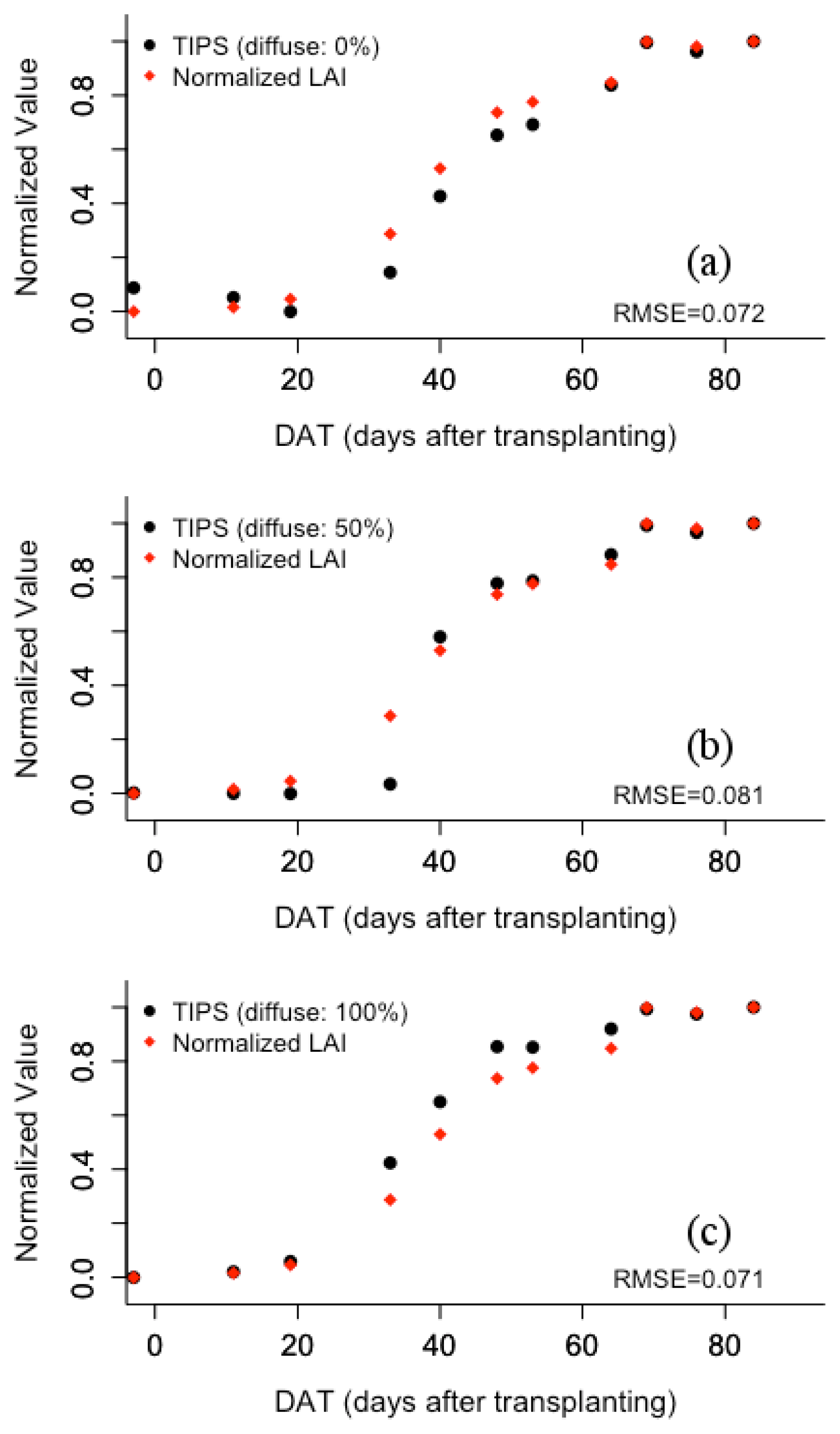
2.3. Validation of the Performance of TIPS under Several Light Conditions

Oki et al. [18] reported that L_dif in Equation (12), the pre-normalized index of TIPS, was the best vegetation index for estimating changes over time in the value of rice LAI under several LAI–vegetation-coverage relationships. This conclusion was reached by comparison with other representative vegetation indices. The canopy reflectances used for calculating vegetation indices in [18] were simulated by the Forest Light Environment Simulator (FLiES) [28]. This simulator can compute reflectance at the top of a heterogeneous plant canopy. Although this is not the result of TIPS, it is considered that the same result will be obtained when TIPS is used instead of L_dif because L_dif is the pre-normalized index of TIPS. That study indicates that TIPS has the potential to provide an accurate estimate of rice LAI without the influence of vegetation coverage. However, this result was obtained under the clear sky condition only. Therefore, before analysis with the field measurement data in this study, the performance of TIPS was verified by FLiES under several light conditions. To verify the performance of TIPS, the parameter values in

Table 2. Parameters used for Forest Light Environment Simulator (FLiES).

Parameter	Value
Fraction of diffuse radiation	0%, 50%, 100%
Solar zenith angle	Calculated from location and observation date
Reflectances of leaf	Blue: 0.049, Green: 0.152, Red: 0.059, NIR: 0.469
Transmittances of leaf	Blue: 0.171, Green: 0.192, Red: 0.160, NIR: 0.456
Reflectances of background *	Blue: 0.074, Green: 0.090, Red: 0.101, NIR: 0.103
Leaf area density	Derived from leaf area index measured on each observation data
Seeding density	28 seedlings/m2

^*Condition of background was shallow water surface on mud.

were used for simulation by FLiES.

For simulating reflectance at the top of a rice canopy, three light conditions were set (fraction of diffuse radiation: 0%, 50%, and 100%). By using a Leaf Clip and Plant Probe (ASD Inc., Lincoln, NE, USA) with FieldSpec 3 spectroradiometer, reflectance and transmittance of leaves were measured 53 days after transplanting in 2008. Background reflectance was measured 3 days before transplanting in 2008 by a FieldSpec 3 spectroradiometer. Solar zenith angles for each day were calculated from the position of the observed paddy field and the observation time and date. Leaf area densities for each day were calculated from LAI measured in each experiment in 2008. Seedling density was obtained from actual rice planting in 2008. Figure 1 shows the simulation results for TIPS behavior with increasing values of LAI on paddy field, as derived from FLiES. This figure indicates that TIPS can be used to monitor changes over time in the value of rice LAI under various light conditions.

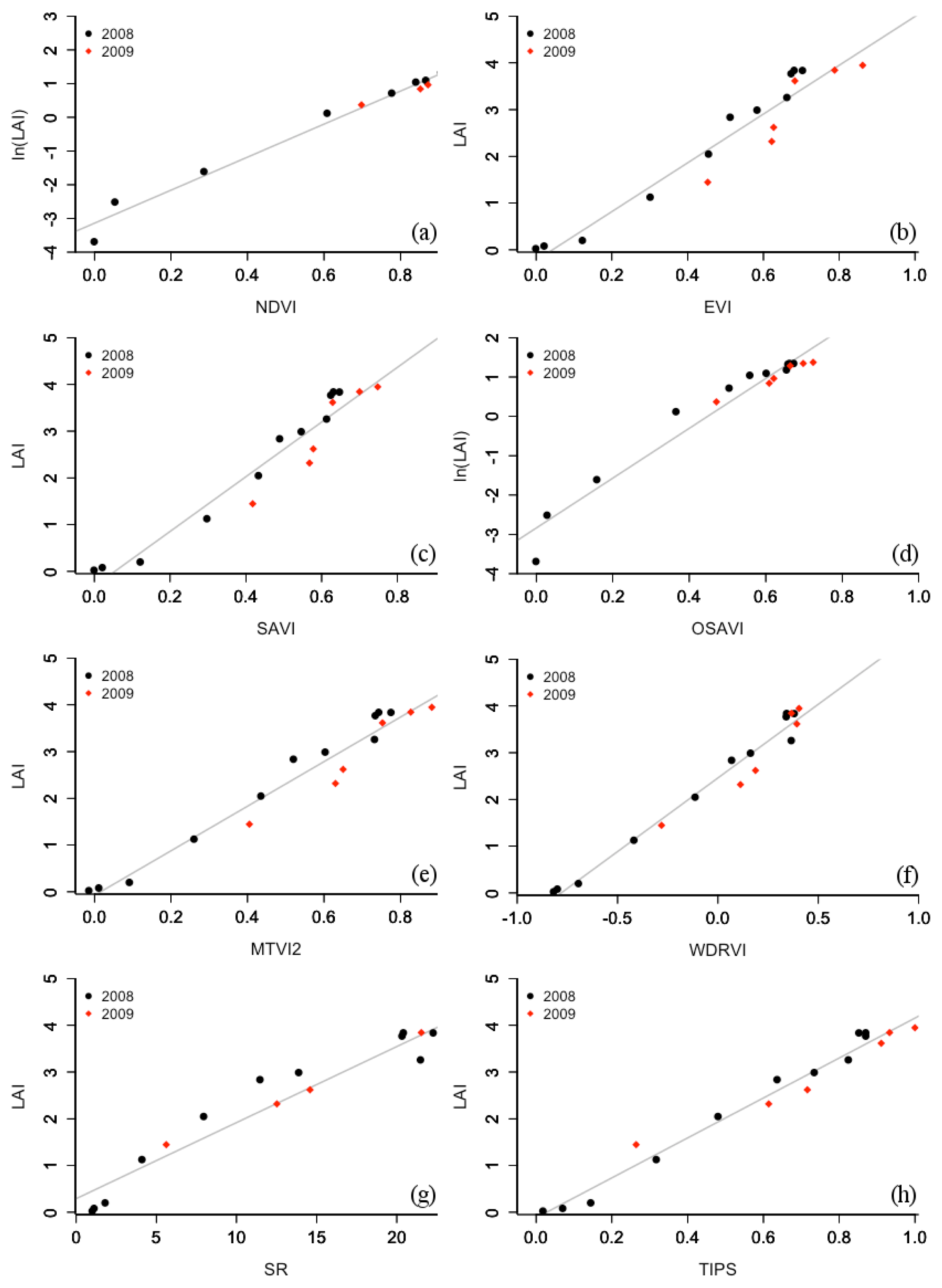
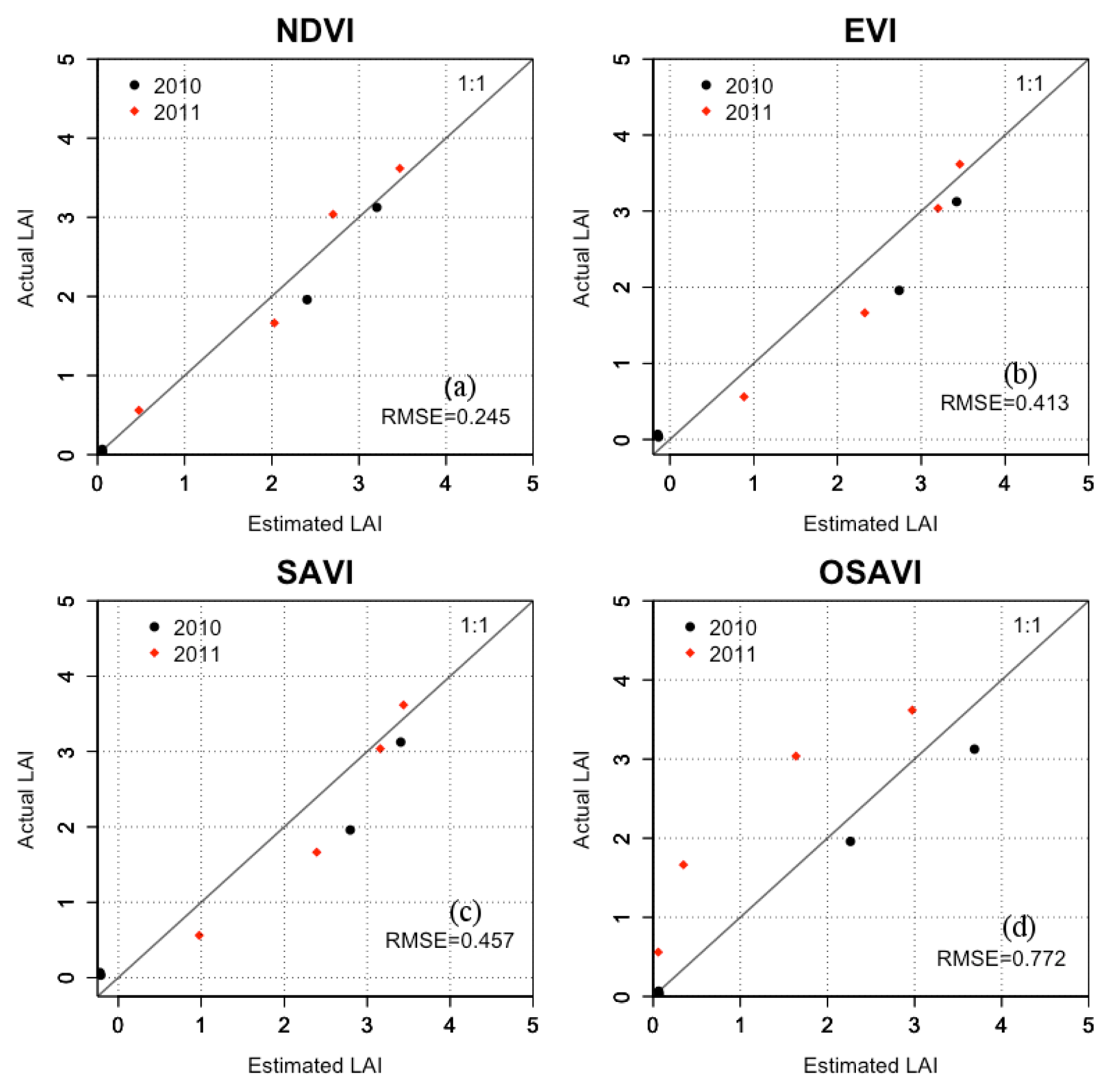
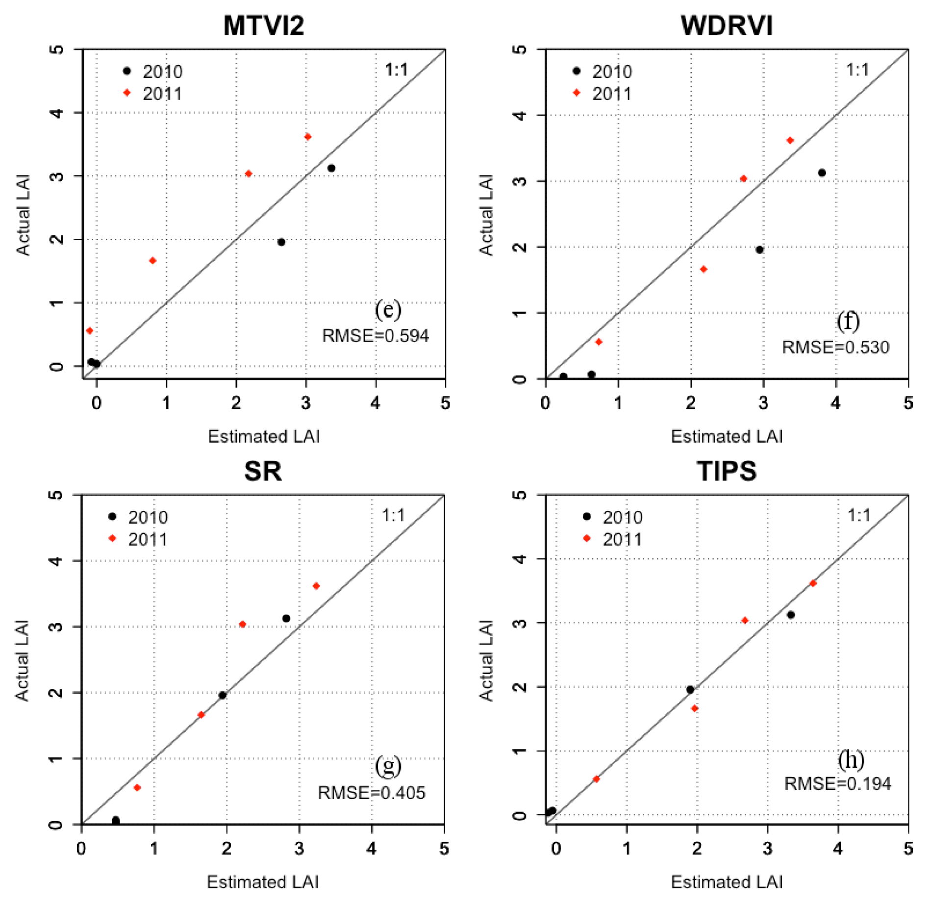
2.4. Analysis Procedure

The results in Section 2.3 indicate that TIPS is more suitable than other vegetation indices for obtaining an accurate estimate of rice LAI if the pure spectral reflectance can be used to calculate TIPS. However, it is difficult to estimate LAI in real time during the growth season in the target period from the pure spectral reflectance of that same period because pure spectral reflectance usually appears during the heading period (at the end of the growth season). Therefore, the ability of TIPS to provide an accurate estimate of LAI in real time during the target period from spectral reflectance data measured in previous experiments was evaluated by the following procedures. (i) The equation for LAI estimation based on TIPS was derived from the LAI–TIPS relationship in 2008 and 2009. In this regard, the pure spectral reflectance was obtained by comparing the values of LAI for 2008 and 2009, and the maximum value at each wavelength across 2008 and 2009 was selected as max (p_k) in Equation (9); (ii) Regression equations for LAI with other vegetation indices were also derived from data obtained in 2008 and 2009; (iii) To estimate LAI, these equations were applied to the data obtained in 2010 and 2011; (iv) The root mean square error (RMSE) of estimated LAI values for 2010 and 2011 were calculated for each vegetation index; (v) By comparing the RMSEs for each vegetation index, the suitability of TIPS for estimating LAI was evaluated. Here, hyperspectral reflectances measured at the experimental farm were converted into wavelength band reflectances that corresponded to the bands of Terra/MODIS. This was done because Terra/MODIS is one of the most commonly used satellite sensors for global monitoring.

In this study, aggregated data for 2008 and 2009 were used in estimating the equation, and aggregated data for 2010 and 2011 were used in verifying the estimated equation because only a small amount of measured LAI and spectral reflectance data were available for each year.

3. Results and Discussion

Table 3. Estimated regression equations for each vegetation index in 2008 and 2009. Values in parentheses (r²) are coefficients of determination.

Vegetation Index	Estimated Equation
NDVI	ln(LAI) = 4.896 × NDVI − 3.136 (r2 = 0.982)
EVI	LAI = 5.219 × EVI − 0.227 (r2 = 0.925)
SAVI	LA I = 5.852 × SAVI − 0.317 (r2 = 0.930)
OSAVI	ln(LAI) = 6.335 × OSAVI − 2.838 (r2 = 0.951)
MTVI2	LAI = 4.769 × MTVI2 − 0.0759 (r2 = 0.957)
WDRVI	LAI = 3.153 × WDRVI + 2.461 (r2 = 0.971)
SR	LAI = 0.164 × SR + 0.291 (r2 = 0.936)
TIPS	LAI = 4.273 × TIPS + 0.119 (r2 = 0.975)

shows the estimated equations for the relationships between LAI and each vegetation index for 2008 and 2009; these are plotted in Figure 2. Values in parentheses (r²) show the coefficients of determination. The results indicate that all indices are closely related to LAI for data from both 2008 and 2009 (r² > 0.9) and, thus, have high potential to provide accurate estimate of the spatial distribution of LAI value if these estimated equations are applied to the place and time when field surveys were conducted. Here, NDVI and OSAVI were logarithmized to obtain a linear approximation, which is the form obtained for other indices. For the calculation of WDRVI, a weight of 0.1 was assigned to α because a strong linear relationship was obtained when this value was used. Typically, nonlinear regression is used to estimate the equations of the relationships between LAI and each vegetation index, but linear regression was used in this study because the resulting coefficients of determination were very high for all expressions. To calculate TIPS from the spectral reflectances measured in 2008 and 2009, the respective spectral reflectances on 26 May 2008 (−3 DAT) and 7 August 2009 (68 DAT) were used as the maximum reflectances for the visible and near-infrared regions, respectively. The spectral reflectance on 7 August 2009 was used as the reference reflectance (pure reflectance of rice canopy). The values for these dates were chosen because among all data for 2008 and 2009, the spectral reflectance in the visible region was highest on 26 May 2008 and the spectral reflectance in near-infrared region was highest on 7 August 2009. The reference reflectance was taken as the value on 7 August 2009 because LAI on this date was at the maximum value among all data for both 2008 and 2009.

Figure 3 shows the results of comparison between actual LAI and estimated LAI for the regression equations in Table 3. This figure indicates that the RMSEs for TIPS and NDVI are smaller than those for other vegetation indices, with the RMSE for TIPS being the smallest of all. In addition to this result, L_dif (the pre-normalized index of TIPS) can better estimate rice LAI under several LAI–AIhe pre-normalized relationships derived from simulation with FLiES than other representative vegetation indices can [18]. The main reason for this is the change of spectral characteristic as rice grows. Although reflectances in both the visible and the near-infrared regions during the early rice-growing period are dominated by surface reflection, reflectance is mainly dominated by surface reflection in the visible region and both surface reflection and multi-scattering in the near-infrared region. When vegetation indices other than TIPS are calculated using these reflectances, those vegetation indices will include the influence of both the surface and canopy layer during the middle and late growing period. That is, these indices will be affected by both LAI and vegetation coverage. In contrast, in calculation of TIPS, information mainly about LAI will be obtained because the influence of surface reflection will be eliminated by Equation (12). From this, the estimated equations for vegetation indices other than TIPS might include influences other than LAI, such as vegetation coverage, for 2008 and 2009. This means that TIPS is relatively more suitable than other vegetation indices for estimating LAI for 2010 and 2011 by the estimated equation derived from 2008 and 2009 data because TIPS reflects information mainly about LAI. As a result, in this study, the maximum spectral reflectances used for regressing LAI on TIPS from data for 2008 and 2009 were the maximum spectral reflectances among data for all years in the study, and the reference reflectances used for the same estimated equation were suitable for use as reference reflectances for LAI estimation in 2010 and 2011 because the LAI value during the heading period in 2009 was the largest among data for all years in the study.

As mentioned above, it is considered that the estimated equation for TIPS derived from previous data should be suitable for estimating LAI during an arbitrary period unless the maximum and the reference reflectances used for the estimated equation are updated during the target period. If one of those reflectances will be updated during the target growing season, it is considered that the estimated equation for TIPS used for previous growing season is not able to retrieve successful result for the target growing season because p′ in Equation (9) or α_vis+nir in Equation (11) can not be correctly calculated. Therefore, it is necessary to monitor whether the maximum spectral reflectances and the reference reflectances are updated before applying the estimated equation for TIPS.

In general, spectral reflectances in the visible region will reach a maximum before transplanting. In particular, the reflectance at blue wavelengths will reach a maximum when water exists on paddy field without crop. The reflectances at green and red wavelengths will reach a maximum when soil exists on a paddy field with neither water nor crop. The reflectance at near-infrared wavelengths will reach a maximum when both LAI and the vegetation coverage on paddy field are at maximum (i.e., the heading period). Therefore, it is possible to confirm whether maximum spectral reflectances in the visible region may be updated before the target growing season. Yearly variations of maximum spectral reflectances in the visible region are likely to be small because the target objects are water and soil. However, the maximum spectral reflectance in the near-infrared region cannot be neglected because that value will change in response to annual rice growing conditions. As with the maximum spectral reflectance in the near-infrared region, reference reflectances will be obtained during the heading period and will change according to each year’s rice growing conditions. Monitoring of the maximum spectral reflectance in the near-infrared region and reference reflectances is the most important determinant for estimation of rice growth by using TIPS. However, it is impossible to confirm whether the reflectances used for TIPS are valid until the heading period. When the maximum spectral reflectance in the near-infrared region and the reference reflectances are updated during the target growing season, then, although TIPS values cannot be compared between those calculated from the old and new normalized spectral reflectances (p′), it will be possible to obtain exact LAI values by the following procedures. (i) The maximum spectral reflectances in the visible region should be confirmed to verify that the values are valid before calculating TIPS of the target growing season; (ii) For the values to be valid, LAI should be obtained by the estimated equation derived from previous data except when α_vis+nir derived from Equation (11) exceeds 1; (iii) If the values are invalid, LAI should be retrieved from the new estimated equation derived from the relationship between LAI measured in previous field surveys and the corresponding TIPS values, which should be updated using the new maximum reflectance (max(p)) in the visible region unless α_vis+nir exceeds 1; (iv) When α_vis+nir exceeds 1, the estimated equation should be recalculated by using the relationship between LAI measured in previous field survey and the corresponding TIPS values, updated with new reference reflectances (m′). Then, LAI can be obtained from this new estimated equation. New reference reflectances should be replaced by the measured reflectances when α_vis+nir exceeds 1 because the reflectances measured at that time reflect information about larger LAI and purer rice canopy than the previous reference reflectances do.

For the above reasons, the proposed method is suitable for areas where LAI and the corresponding spectral reflectances have been previously measured. It is not possible to apply the method to areas where LAI and the corresponding spectral reflectances have not been previously measured.

4. Conclusions

Several vegetation indices were tested for estimating the rice LAI across several years at the field scale. In particular, the suitability of TIPS, a vegetation index developed for monitoring changes in the value of LAI over time, was evaluated by comparison with other vegetation indices. Estimated equations for LAI were derived from the relationships between LAI and each vegetation index on the basis of 2008 and 2009 data. These estimated equations were subsequently applied to estimate LAI from spectral reflectances measured in 2010 and 2011. TIPS and NDVI estimated LAI in 2010 and 2011 more accurately than the six other vegetation indices. Moreover, it was reported that L_dif (the pre-normalized index of TIPS) more accurately estimated rice LAI under several LAIce LAI under several relationships than other indices did, especially in the rapid growing period [18]. Therefore, it is considered that TIPS is more suitable than other representative vegetation indices for estimating rice LAI across several years. The reason for this is that TIPS reflects mainly information about LAI; other indices reflect information about not only LAI but also other parameters, such as vegetation coverage, height, and density. From abovementioned results, it is considered that this study could propose the LAI estimation method using vegetation index (TIPS) that can estimate rice LAI in arbitrary year without field measurement in the same year if LAI and spectral measurements had been conducted through growing season in past times. Although the utilization of TIPS was not completely validated, it is thought that the results obtained from this study can contribute to reduce effort and expense of field measurement for LAI estimation using spectral information at field scale.

To ensure stable utilization of TIPS for the real-time estimation of LAI at the field scale, a collection of rice canopy reflectances under various growth conditions will be investigated in future studies. Toward this end, measuring the spectral reflectance, vegetation coverage, and LAI is recommended when field surveys are conducted. The suitability of TIPS for estimating LAI of other major crops, such as maize and soybean, should also be verified in future studies. Moreover, to monitor rice growth at the regional and global scales, it is necessary to verify the suitability of TIPS derived from satellite data, such as Terra/MODIS data, and assess the suitability of the relationship between LAI and spectral reflectances simulated by radiative transfer models for calculating TIPS and the estimated equation of LAI for each area.

Finally, under the assumption that hyperspectral imagery can be widely used for regional and global monitoring, in order to improve TIPS, it will be necessary to verify the suitability of the partial least squares regression and red-edge inflection point methods in the near future because those methods are representative of methods for retrieving biophysical variables, such as biomass and LAI, from hyperspectral data.

References

1. Dente, L.; Satalino, G.; Mattia, F.; Rinaldi, M. Assimilation of leaf area index derived from ASAR and MERIS data into CERES-wheat model to map wheat yield. Remote Sens. Environ 2008, 112, 1395–1407. [Google Scholar]
2. Fang, H.; Liang, S.; Hoogenboom, G.; Teasdale, J.; Cavigelli, M. Corn-yield estimation through assimilation of remotely sensed data into the CSM-CERES-Maize model. Int. J. Remote Sens 2008, 29, 3011–3032. [Google Scholar]
3. Curnel, Y.; de Wit, A.; Duveiller, G.; Defourny, P. Potential performances of remotely sensed LAI assimilation in WOFOST model based on an OSS experiment. Agric. For. Meteorol 2011, 151, 1843–1855. [Google Scholar]
4. Padilla, F.L.M.; Maas, S.J.; González-Dugo, M.P.; Mansilla, F.; Rajan, N.; Gavilán, P.; Dominguez, J. Monitoring regional wheat yield in southern Spain using the GRAMI model and satellite imagery. Field Crops Res 2012, 130, 145–154. [Google Scholar]
5. Xiao, X.; He, L.; Salas, W.; Li, C.; Moore, B., III; Zhao, R.; Frolking, S.; Boles, S. Quantitative relationships between field-measured leaf area index and vegetation index derived from VEGETATION images for paddy rice field. Int. J. Remote Sens 2002, 23, 3595–3604. [Google Scholar]
6. Bsaibes, A.; Courault, D.; Baret, F.; Weiss, M.; Olioso, A.; Jacob, F.; Hagolle, O.; Marloie, O.; Bertrand, N.; Desfond, V.; Kzemipour, F. Albedo and LAI estimation from FORMOSAT-2 data for crop monitoring. Remote Sens. Environ 2009, 113, 716–729. [Google Scholar]
7. Hansen, P.M.; Schjoerring, J.K. Reflectance measurement of canopy biomass and nitrogen status in wheat crops using normalized difference vegetation indices and partial least squares regression. Remote Sens. Environ 2003, 86, 542–553. [Google Scholar]
8. Darvishzadeh, R.; Skidmore, A.; Schlerf, M.; Atzberger, C.; Corsi, F.; Cho, M. LAI and chlorophyll estimation for a heterogeneous grassland using hyperspectral measurements. ISPRS J. Photogramm. Remote Sens 2008, 63, 409–426. [Google Scholar]
9. Knyazikhin, Y.; Martonchik, J.V.; Myneni, R.B.; Diner, D.J.; Running, S.W. Synergistic algorithm for estimating vegetation canopy leaf area index and fraction of absorbed photosynthetically active radiation from MODIS and MISR data. J. Geophys. Res 1998, 103, 32257–32276. [Google Scholar]
10. Baret, F.; Hagolle, O.; Geiger, B.; Bicheron, P.; Miras, B.; Huc, M.; Berthelot, B.; Niño, F.; Weiss, M.; Samain, O.; et al. LAI, fAPAR and fCover CYCLOPES global products derived from VEGETATION. Part 1: Principles of the algorithm. Remote Sens. Environ 2007, 110, 275–286. [Google Scholar]
11. Darvishzaden, R.; Atzberger, C.; Skidmore, A.; Schlerf, M. Mapping grassland leaf area index with airborne hyperspectral imagery: A comparison study of statistical approaches and inversion of radiative transfer models. ISPRS J. Photogramm. Remote Sens 2011, 66, 894–906. [Google Scholar]
12. Atzberger, C.; Richter, K. Spatially constrained inversion of radiative transfer models for improved LAI mapping from future Sentinel-2 imagery. Remote Sens. Environ 2012, 120, 208–218. [Google Scholar]
13. Huete, A. A soil-adjusted vegetation index (SAVI). Remote Sens. Environ 1988, 25, 295–309. [Google Scholar]
14. Rondeaux, G.; Steven, M.; Baret, F. Optimization of soil-adjusted vegetation indices. Remote Sens. Environ 1996, 55, 95–107. [Google Scholar]
15. Haboudane, D.; Miller, J.R.; Pattey, E.; Zarco-Tejada, P.J.; Strachan, I.B. Hyperspectral vegetation indices and novel algorithms for predicting green LAI of crop canopies: Modeling and validation in the context of precision agriculture. Remote Sens. Environ 2004, 90, 337–352. [Google Scholar]
16. Liu, H.Q.; Huete, A. A feedback based modification of the NDVI to minimize canopy background and atmospheric noise. IEEE Trans. Geosci. Remote Sens 1995, 33, 457–465. [Google Scholar]
17. Gitelson, A.A. Wide dynamic range vegetation index for remote quantification of biophysical characteristics of vegetation. J. Plant Physiol 2004, 161, 165–173. [Google Scholar]
18. Oki, K.; Noda, K.; Yoshida, K.; Azechi, I.; Maki, M.; Homma, K.; Hongo, C.; Shirakawa, H. Development of an Environmentally Advanced Basin Model in Asia. In Crop Production, 1st ed; Goyal, A., Asif, M., Eds.; InTech: Rijeka, Croatia, 2013; pp. 17–48. [Google Scholar]
19. Liu, J.; Jégo, G. Assessment of vegetation indices for regional crop green LAI estimation from Landsat images over multiple growing seasons. Remote Sens. Environ 2012, 123, 347–358. [Google Scholar]
20. Hashimoto, N.; Maki, M.; Tanaka, K.; Tamura, M. Study of a method for extracting LAI time-series patterns for estimation of crop phenology. J. Remote Sens. Soc. Jpn 2009, 29, 381–391, (In Japanese with English abstract). [Google Scholar]
21. Lillesaeter, O. Spectral reflectance of partly transmitting leaves-laboratory measurements and mathematical modelling. Remote Sens. Environ 1982, 12, 247–254. [Google Scholar]
22. Baret, F.; Guyot, G. Potentials and limits of vegetation indexes for LAI and APAR assessment. Remote Sens. Environ 1991, 35, 161–173. [Google Scholar]
23. Huete, A.; Liu, H.; Batchily, K.; van Leeuwen, W. Comparison of vegetation indices over a global set of TM images for EOS-MODIS. Remote Sens. Environ 1997, 59, 440–451. [Google Scholar]
24. Huete, A.; Didan, K.; Miura, T.; Rodriguez, E.P.; Gao, X.; Ferreira, L.G. Overview of the radiometric and biophysical performance of the MODIS vegetation indices. Remote Sens. Environ 2002, 83, 195–213. [Google Scholar]
25. Steven, M. The sensitivity of the OSAVI vegetation index to observational parameters. Remote Sens. Environ 1998, 63, 49–60. [Google Scholar]
26. Gitelson, A.A.; Wardlow, B.D.; Keydan, G.P.; Leavitt, B. An evaluation of MODIS 250-m data for green LAI estimation in crops. Geophys. Res. Lett 2007, 34. [Google Scholar] [CrossRef]
27. Oki, K.; Oguma, H. Estimation of the canopy coverage in specific forest using remotely sensed data—Estimation of Alder trees in Kushiro Mire. J. Remote Sens. Soc. Jpn 2002, 22, 510–516, (In Japanese with English abstract). [Google Scholar]
28. Kobayashi, H.; Iwabuchi, H. A coupled 1-D atmosphere and 3-D canopy radiative transfer model for canopy reflectance, light environment, and photosynthesis simulation in a heterogeneous landscape. Remote Sens. Environ 2008, 112, 173–185. [Google Scholar]
Figure 1. Simulation results of TIPS behavior with increasing values of LAI on a paddy field, as derived from FLiES. The panels show the results with diffuse radiations of (a) 0%, (b) 50%, and (c) 100%, respectively.
Remotesensing 06 04764f1
Figure 2. Relationship between LAI and each vegetation index in 2008 and 2009. (a) NDVI; (b) EVI; (c) SAVI; (d) OSAVI; (e) MTVI2; (f) WDRVI; (g) SR; (h) TIPS.
Remotesensing 06 04764f2
Figure 3. Comparison of results for actual LAI and estimated LAI. (a) NDVI; (b) EVI; (c) SAVI; (d) OSAVI; (e) MTVI2; (f) WDRVI; (g) SR; (h) TIPS.
Remotesensing 06 04764f3aRemotesensing 06 04764f3b