Semi-Supervised Learning for Ill-Posed Polarimetric SAR Classification

Abstract

In recent years, the interest in semi-supervised learning has increased, combining supervised and unsupervised learning approaches. This is especially valid for classification applications in remote sensing, while the data acquisition rate in current systems has become fairly large considering high- and very-high resolution data; yet on the other hand, the process of obtaining the ground truth data may be cumbersome for such large repositories. In this paper, we investigate the application of semi-supervised learning approaches and particularly focus on the small sample size problem. To that extend, we consider two basic unsupervised approaches by enlarging the initial labeled training set as well as an ensemble-based self-training method. We propose different strategies within self-training on how to select more reliable candidates from the pool of unlabeled samples to speed-up the learning process and to improve the classification performance of the underlying classifier ensemble. We evaluate the effectiveness of the proposed semi-supervised learning approach over polarimetric SAR data. Results show that the proposed self-training approach using an ensemble-based classifier that is initially trained over a small training set can achieve a similar performance level of a fully supervised learning approach where the training is performed over significantly larger labeled data. Considering the difficulties of the manual data labeling in such massive volumes of SAR repositories, this is indeed a promising accomplishment for semi-supervised SAR classification.

1. Introduction

Classification using machine-learning approaches is commonly used over remote sensing data in various applications. Generally, supervised learning (SL) approaches are able to achieve better results than unsupervised learning (UL) methods due to incorporating prior knowledge in the form of ground truth data. Yet at the same time, this can be considered a drawback since SL requires labeled training data normally provided manually by a human expert. Even though this is probably the situation for the majority of fields to which SL is applied, it is particularly the case for remote sensing data classification. The reason is that ideally on-site visits are conducted to the locations from which the remote sensing data has been acquired, especially keeping in mind that SL benefits from larger number of labeled data during training. With a rather limited amount of training data available, the classification task becomes easily ill-posed due to the small sample size problem, where the number of training samples is considered too small in relation to the feature dimension. Due to this, the underlying classifier will lack discrimination and generalization capabilities. This becomes more evident when the classification problems are of more complex nature such as multi-class classification tasks where the number of classes might be equal or higher than the feature dimension.

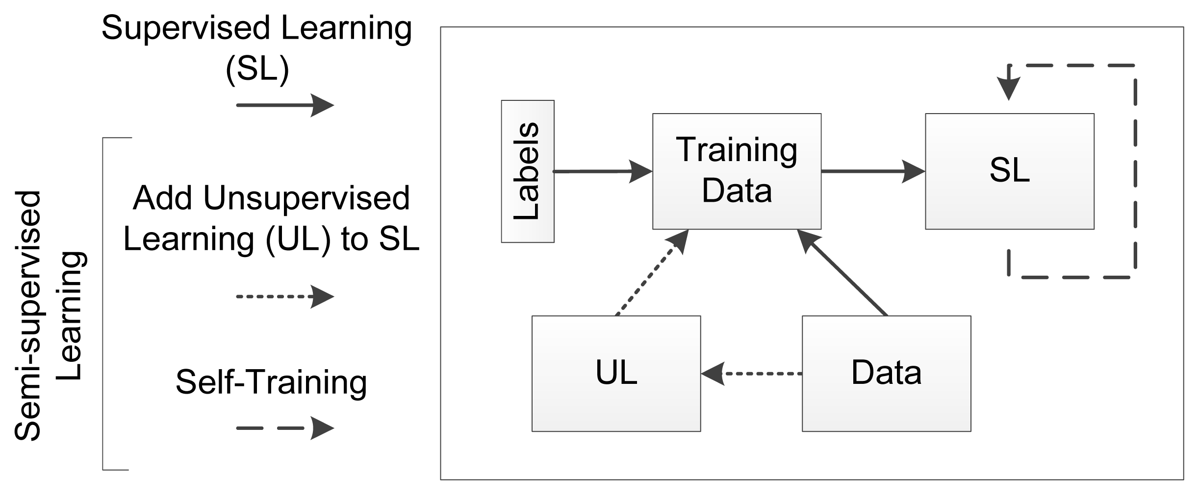
In recent years, the interest in semi-supervised learning (SSL) has increased because it can combine supervised and unsupervised learning approaches. This is especially valid for remote sensing classification applications as the acquired data from current systems are fairly large considering high- and very-high resolution data acquisition requiring more specific surface- or even object-based classification. The general notion behind SSL is to start from a set of labeled data and then to utilize the large amount of unlabeled data to improve the initial classifier [1]. Therefore, the crucial part in this process is the automatic selection of reliable training data among the unlabeled data. This can be performed by several approaches such as unsupervised clustering methods [2,3], using self-training [4] where one initial learner iteratively selects the most confident samples to add them to the training set, or co-training [4] where two classifiers either work on different feature spaces or are completely different altogether and add new training samples to one another. Figure 1 illustrates the relation of typical supervised learning (SL) to SSL, which might encapsulate an UL preceding a SL process or a self-training process over a SL process.

To aid the selection of reliable new training data for SSL, several assumptions [5] are generally exploited where the first two are the most commonly used. Firstly, there is the local smoothness/consistency assumption, where nearby points are more likely to have the same label such that there is a higher probability a point shares the same label with points in its local vicinity. This is the same assumption any SL algorithm exploits to learn from the training data and generalize a model or function applicable to any unseen data provided in the future. Typically, this is performed in the feature space; however, it can also be applied spatially over the neighborhood of each image pixel. Secondly, the global cluster assumption exploiting the fact that points sharing the same structure, hence, would fall into the same cluster are likely to have the same label so that those unlabeled samples which are highly similar to a labeled sample should share its label. This includes approaches based on the low-density separation assumption where in many clustering methods the cluster centers are considered of high-density zones so that the decision boundaries should lie within regions of lower density. In this case, rather than to find the high-density sample regions directly, the focus lies in finding such low-density regions to best draw decision boundaries among clusters. As another assumption, the fitting constraint can be considered where a good classifier should not deviate too much from its initial label assignments during a learning process.

In the area of remote sensing image classification, SSL has recently attracted a lot of attention. Two decades ago, the early investigations showed how unlabeled samples could be beneficial for classification applications [6]. In this work, the authors studied techniques to address the small sample size problem by using unlabeled observations and their potential advantages in enhanced statistic estimation. Their main conclusion was that more information could be obtained and utilized with the additional unlabeled samples. Based on these observations, a self-learning and self-improving adaptive classifier [7] using generative learning was proposed to mitigate the small sample size problem that can severely affect the recognition accuracy of classifiers. To accomplish this in [7], they iteratively utilized a weighted mixture of labeled and semi-labeled samples.

Following these pioneer works, there have been various SSL approaches over remote sensing data such as generative learning in form of semi-supervised versions of a spatially adaptive mixture-of-Gaussians model was proposed in [8,9]. Another approach uses graph-based methods, which rely upon the construction of a graph representation [10], where vertices are the labeled and unlabeled samples and edges represent the similarity among samples in the dataset including, for example, contextual information via composite kernels [11]. Furthermore, this graph-based approach was also employed within self-training, where the graph is used to assure reliability of newly added training examples [12,13]. However, the general issue of graph-based methods is that the label propagation relies on the inversion of a large matrix with a size equivalent of the total number of labeled and unlabeled pixels, which limits their application for remote sensing applications.

One of the most basic semi-supervised learning approaches is to consider the output of an unsupervised learning method as the input of a supervised learning approach. This has been applied to SAR images where unsupervised clustering in form of Deterministic Annealing was used as the training input for a Multi-Layer Perceptron [2]. This type of combined approach has also been used with other classifier types such as Support Vector Machines (SVMs) using the output of the fuzzy C-means (FCM) clustering, which was further extended by Markov Random Fields exploiting contextual information from multiple SVM-FCM classification maps [3]. A similar approach to the combination of supervised and unsupervised learning algorithms is the application of cluster kernels [14,15] employing SVM, where so-called bagged kernels are used to encode the similarity between unlabeled samples obtained via multiple runs of unsupervised k-means clustering.

Furthermore, SVM has been used within the context of self-training, where a binary transductive SVM has been adapted in a one-against-all topology [16]. Besides that, one-class SVM has been applied to detect pixels belonging to one of the classes in the image and reject the others [17]. Yet another semi-supervised SVM approach utilizes the so-called context-pattern in a form of 4- or 8-connected pixel neighborhoods to identify possible misleading initial training labels [18]. Besides its popularity, the application of SVMs in the semi-supervised learning context has some shortcomings such as particularly high computational complexity, utilization of a non-convex cost function, and the usage of multiclass SVMs. These shortcomings have been addressed by using semi-supervised logistic regression algorithm [19] and by replacing the SVMs with an artificial neural network [20] offering much better scalability than SVM-based methods.

In the case of supervised learning, combining multiple classifiers to a committee or ensemble has demonstrated to improve classification performance over single classifier systems [21] and its effectiveness has also been shown for remote sensing data [22]. Generally, ensemble learning tries to improve generalization by combining multiple learners, whereas semi-supervised learning attempts to achieve strong generalization by exploiting the unlabeled data. Hence, fusing these two learning paradigms, even stronger learning systems can be generated by leveraging unlabeled data and classifier combination [23]. Zhou and Li proposed the Tri-training approach [24], which can be considered an extension of the co-training algorithms, where three classifiers are used and when two of them agree on a label of an unlabeled sample while the third disagrees; then, under a certain condition, the two classifiers will label this unlabeled sample for the training of the third classifier. Later, Tri-training was extended to Co-forest [25] including more base classifiers adopting the “majority teaches minority” strategy. Additionally, semi-supervised boosting methods have been proposed such as Assemble [26], which labels unlabeled data by the current ensemble and iteratively combines semi-labeled samples with the original labeled set to train a new base learner which is then added to the ensemble. The more generic SemiBoost [27] combines classifier confidence and pairwise similarity to guide the selection of unlabeled examples. Bagging and boosting based ensemble approaches became popular within SSL, particularly self-training, with a general outline illustrated in Scheme 1; however, they are not much adapted to remote sensing data as for other areas.

The general ensemble-based outline as given in Scheme 1 was utilized by an approach named Semi-labeled Sample Driven Bagging using Multi-Layer Perceptron [28] and k-Nearest Neighbor [29] classifiers over multispectral data. Furthermore, ensembles have been applied to the concept of unsupervised learning where the Cluster-based ENsemble Algorithm [30] applies Mixture of Gaussians (MoG) and support cluster machine to attack the quality problems of the training samples. In this case, the ensemble technique is used to find the best number of components going from coarse to fine to generate different sets of MoG. A self-trained ensemble with semi-supervised SVM has been proposed in [31] for pixel-based classification where fuzzy C-Means clustering is employed to obtain confidence measures for unlabeled samples, which are then used in an ensemble of SVMs. Here, each SVM classifier starts with a different training set, which might be difficult within a small sample size problem when the initial labeled training data cannot be divided into multiple partitions.

There have been quite many SSL investigations over spectral-based remote sensing data where only a few particularly focused on ill-posed classification of the small sample size problem, which makes the selection of the initial training dataset more critical [32]. However, SSL has not yet been considered in such a high scale that the polarimetric SAR (PolSAR) data reside particularly when it comes to the evaluation of the classification performance. In this study, the main questions that we shall tackle are: (1) how small can the initially labeled training set be to still achieve good results, with and without SSL? (2) while applying SSL initially with small size training data, is it possible to reach similar accuracies to a SL approach that is trained over a significantly larger dataset regardless from the number of iterations or unlabeled samples? With these two questions in mind, we focus on three main investigations regarding the small sample size problem over polarimetric SAR data. Firstly, before applying self-training we shall consider an unsupervised and a supervised approach to enlarge the initial user-annotated training data as an initial stage of the SL. Secondly, we shall investigate a bagging ensemble approach through combining the advantages of a multi-classifier system with semi-supervised learning. Thirdly, we shall consider different strategies within the self-training procedure on how to select from the pool of unlabeled samples to speed-up the learning process and also to improve both generalization and classification performance.

The rest of the paper is organized as follows. We introduce our semi-supervised ensemble scheme along with the proposed modifications in Section 2. Section 3 covers the PolSAR image data, internal parameters used and the experimental setup of the base classifiers used in the ensemble. Section 4 provides comparative evaluations and classification results over the PolSAR image dataset. Finally, Section 5 concludes the paper and discusses topics for future work.

2. Semi-Supervised Learning Approaches

In general, semi-supervised learning approaches employing ensemble classifiers are straightforward and proven effective. We adopt the bagging ensemble approach similar to Chi and Bruzzone [28,29] as our underlying supervised learning approach since such systems are generally classifier independent and advantageous against SVM and graph-based methods regarding memory requirements especially for larger data.

The general outline of a bagging ensemble is to start with a small training set. As the first step, a base learner h is trained with labeled training set, L, and added to the ensemble H. At step t, the unlabeled data, U, is classified and as a result, semi-labels based on confidence values from H_t−1 are obtained. As in [28,29], a subset SL_t from U is then extracted, containing the pixels that are randomly selected from the unlabeled samples over the entire image for a better spatial distribution. The pixels should have a confidence score above a certain level (e.g., 0.85 for the Multi-Layer Perceptrons) and a total number of twice the amount of labeled samples is selected. Then a new base learner h is trained using L and SL_t and added to H_t, i.e., H_t = H_t−1 + h(L, SL_t). This is an iterative process until a predefined number (such as 20) of classifiers in H is reached. They employed k-nearest neighbor and Multi-Layer Perceptrons as the base learners and penalized the unlabeled samples using the confidence values obtained from the previous ensemble H_t−1. This is done so the semi-labels selected among the unlabeled samples do not have the same influence during training as the labeled samples. For the k-Nearest Neighbor, the penalty is applied when the nearest neighbors are compared while classifying a sample, whereas in case of Multi-Layer Perceptrons, they modified the mean squared error cost function instead.

We use the aforementioned ensemble approach within a self-training process executed in our semi-supervised learning setup. In addition, we propose three modifications to improve the classification accuracy and to reduce the number of self-training iterations required. The modifications to the general ensemble approach are highlighted in Scheme 2 and each modification is described as follows:

(1)

We employ unsupervised clustering as a pre-stage to tackle the small training set problem, which is a regular starting point in a SSL scenario. The main idea is that any option that is able to extend the training set accurately would be highly beneficial since a better generalization and hence a superior classification performance can be achieved over a larger training dataset. Here a straightforward approach is to use the contextual information within the pixel neighborhood of the labeled samples and assign the same label to the neighbors. By employing this contextual information in form of the 4- or 8-connected neighbors, we shall exploit a local spatial smoothness and consistency among the image pixels. This way we can easily enlarge the initial training set by 4- or 8-times with a high probability of the semi-labeled neighbors having the correct label. To further increase the number of training samples, we can compute a dense over-segmentation of an image, applying a superpixel [33] segmentation approach. This segments the image into small homogenous regions, the so-called superpixels [33], respecting local image boundaries, while limiting under-segmentation through a compactness constraint. Again, this is a spatial smoothness and consistency among pixel intensities. Compared to the connected neighbors approach, this may properly extend the initial training set by an order of magnitude depending on the average size of the obtained superpixels. However, the outcome will be parameter dependent with respect to the size and compactness of the superpixel algorithm, which might also affect the accuracy of the semi-labels.

(2)

Within our self-training process, we employ a bagging ensemble as the underlying supervised learning approach, which relies on a base classifier. It is a commonly known that employing a strong classifier for any supervised learning is advantageous. Therefore, we exploit the fact that combining multiple classifiers to a committee or ensemble has shown to improve classification performance over single classifier systems [21].

(3)

In any self-training approach, a significant improvement over the classification performance can usually be achieved only by selecting a reliable set of new training samples from the large pool of unlabeled samples. Therefore, rather than selecting them from the entire image excluding the ground truth, we can limit the search neighborhood to the vicinity of the provided labeled samples. This neighborhood exploits a spatial smoothness constraint at the beginning and the area of which can be increased with each iteration. In the proposed approach we consider how and where to select unlabeled samples in the following way.

The how is usually measured by the (class) confidence values provided by the classifier, i.e., computing the confidence score of each sample belonging to a particular class. Via a confidence threshold (THR) applied to the class confidence values we can determine which unlabeled samples should be selected among the unlabeled data. The rule of thumb is that we want to pick samples above a certain class confidence value to ensure not adding and accumulating too much error. However, the drawback of choosing the threshold too high is the selection of such samples that were already learned by the classifier. Thus, they will not add any new information to the ongoing learning process; hence, we want certain amount of diversity among the semi-labeled and labeled samples.

The where indicates the search for the location to select new training data after applying the confidence threshold. This is usually performed over all available unlabeled samples to exploit information presented in the entire data or image. This is a valid approach; however, due to the large amount of unlabeled samples, the selection of the most reliable candidates becomes more difficult especially when we want to add new information to the (self-training) learning process. Due to nature of remote sensing data, we can exploit the spatial location in the close vicinity of the provided labeled data rather than performing some feature clustering methods with unknown distance metrics, both of which can create further uncertainties or erroneous training data selections in the process. Therefore, the main idea is to grow the search neighborhood with the notion that the provided labeled data is correct exploiting the smoothness and consistency assumptions while focusing the selection process among the unlabeled data within a close vicinity of the labeled data. This search strategy has the advantage that the initial classifier may find such unlabeled data that do not necessarily have the highest class confidence values but are able to provide more diversity among the training samples. Especially at the beginning of the self-training process, we are trying to increase the size of the training set with reliable and informative “semi-labeled” samples. Therefore, two options are considered: (1) the search neighborhood is limited to the vicinity around all labeled samples to determine those semi-labeled samples among the unlabeled samples per class, NH_L. This can be considered as a localized version of selecting from the entire image. In addition, (2) setting the search neighborhood around the labeled samples of a particular class to determine the semi-labeled samples per class, NH_C. The search area of those two strategies can iteratively grow with the number of SSL iterations to cover the entire image eventually. We shall consider and evaluate both strategies in the proposed self-training approach.

3. Experimental Setup

This section presents the experimental setup, the polarimetric SAR (PolSAR) data used, and parameters of the bagging ensemble approach.

3.1. Polarimetric SAR Image and Features

For our experiments and comparative evaluations, we selected the Flevoland image from the NASA/Jet Propulsion Laboratory AIRSAR airborne system. The four-look fully polarimetric L-Band data of Flevoland, The Netherlands, was collected in mid-August 1989 during MAESTRO-1 Campaign with a size of 1024 × 750 pixels. This particular region has been extensively used as a test side for crop and land classification over the past years with well-established ground truth data [34] of 15 classes as shown in Figure 2. The size of the ground truth data is around 208,000 pixels. The image is speckled filtered [35] with a 5 × 5 window before we apply the HαA eigenvalue decomposition [36].

Based on the coherency matrix, 〈[T]〉, the eigenvalue decomposition applies eigenanalysis such as,

$$\langle [T]\rangle ={\lambda }_1{e}_1{e}_1^{*T}+{\lambda }_2{e}_2{e}_2^{*T}+{\lambda }_3{e}_3{e}_3^{*T}$$

(1)

where λ₁ > λ₂ > λ₃ ≥ 0 are real eigenvalues and the corresponding orthonormal eigenvectors e_i, representing three scattering mechanisms, are

$$e_i=e^{i{\phi }_i}{\left[\text{cos\hspace{0.17em}}{\alpha }_i,\text{sin\hspace{0.17em}}{\alpha }_i\hspace{0.17em}\text{cos\hspace{0.17em}}{\beta }_i{e}^{i{\delta }_i},\text{sin\hspace{0.17em}}{\alpha }_i\hspace{0.17em}\text{sin\hspace{0.17em}}{\beta }_i{e}^{i{\gamma }_i}\right]}^T$$

(2)

Furthermore, Cloude and Pottier defined entropy H, a set of four angle averages ᾱ, β̄, δ̄, and γ̄, and anisotropy A for the analysis of the physical information related to scattering characteristics of a medium as,

$$H=-\sum _{i=1}^n{p}_i\hspace{0.17em}{\text{log}}_n{p}_i\hspace{0.17em}where\hspace{0.17em}{p}_i=\frac{{\lambda }_i}{{\displaystyle \sum _{i=1}^n}{\lambda }_i},$$

(3)

$$\overline{\alpha }=\sum _{i=1}^n{p}_i{\alpha }_i,\mathrm{\hspace{0.17em} }\overline{\beta }=\sum _{i=1}^n{p}_i{\beta }_i,\mathrm{\hspace{0.17em} }\overline{\delta }=\sum _{i=1}^n{p}_i{\delta }_i,\mathrm{\hspace{0.17em} }\overline{\gamma }=\sum _{i=1}^n{p}_i{\gamma }_i,\mathrm{\hspace{0.17em} }A=\frac{p_2-p_3}{p_2+p_3}$$

(4)

with n = 3 for backscatter problems. For a multi-look coherency matrix, the entropy, 0 ≤ H ≤ 1 represents the randomness of a scattering medium between isotropic scattering (H = 0) and fully random scattering (H = 1), while the average angle ᾱ can be related to the target average scattering mechanisms from a single-bounce (or surface) scattering (ᾱ ≈ 0), dipole (or volume) scattering (ᾱ ≈ π/4), and double-bounce scattering (ᾱ ≈ π/2). Due to the basis invariance of the target decomposition, H and ᾱ are roll invariant, hence they do not depend on the orientation of the target in the radar line of sight. Additionally, information about a target’s total backscattered power can be determined by the so-called Span defined as,

$$Span=\sum _{i=1}^3{\lambda }_i$$

(5)

Moreover, Kim and van Zyl introduced an estimation of forest biomass from PolSAR data based on the eigenvalue analysis of the covariance matrix 〈[C]〉, the so-called Radar Vegetation Index (RVI) [37] defined as,

$$RVI=\frac{4\hspace{0.17em}\text{min\hspace{0.17em}}({\lambda }_1,{\lambda }_2,{\lambda }_3)}{{\lambda }_1+{\lambda }_2+{\lambda }_3}$$

(6)

We use 11 features in form of entropy H, anisotropy A, average angles α, β, γ, δ, the three eigenvalues, Span, and the RVI. We have chosen them as the components of HαA and eigenvalue decomposition are commonly used as features in PolSAR classification. Furthermore, in a previous evaluation [38], these features demonstrated superior performances compared to the covariance matrix and various other target decomposition components. However, we do not consider the applied features as critical in the overall process as our objective is not related to the application of particular feature sets and their performance evaluations against each other.

3.2. SSL Ensemble-Driven Approach

The initial labeled training set is critical for semi-supervised learning techniques [32]. To validate this we generate our training datasets T_i in the following manner. We start with training set T₁ where each class has exactly one (i = 1) labeled sample. In the Flevoland dataset there are 15 terrain classes (nC = 15), so that T₁ has a total size of 15. Furthermore, we randomly generated 10 instances of T₁. Now the instances of training set T₂ are created by randomly adding a new and different labeled training sample to each of the 10 instances of T₁ so that T₁ ⊂ T₂ for all instances. Every instance of T₂ now includes two (i = 2) labeled samples per class. We continue this process up to i = 10 so that T₁ ⊂ T₂ ⊂ … ⊂ T₉ ⊂ T₁₀. In total, we end up with 100 training sets with sizes from 15 to 150. With such training dataset formation, we now detail each of the three contributions of our semi-supervised learning approach proposed in Section 2.

(1)

During the pre-stage of the SSL approach, each T_i is enlarged by the 8-connected neighbors around each labeled pixel (NN_i, i.e., see Figure 3(left)) and by the pixels belonging to the same superpixel as the labeled pixels (SP_i). As the outcome shown in Figure 3(right), we employed the TurboPixels algorithm [33] with the (maximum) number of superpixels as 8000 that is empirically determined to get compact and homogeneous superpixels. With this parameter setting, the algorithm will produce 7434 super pixels with an average size of around 103 pixels. As an alternative approach, a more recent algorithm [39] could also be used instead where one just needs to specify the desired superpixel size and its compactness rather than the number of superpixels. Note that the choice of the superpixel algorithm is not critical for this study. Figure 4 shows an example of NN_i and SP_i on an instance of T₅ over a selected area.

(2)

As a base classifier within the self-training stage, we will employ a rather weak classifier in form of a decision tree (DT) algorithm [40] due to its simplicity and parameter independence. Additionally, we will consider Random Forests (RF) [40] as a multi-classifier system of DTs in order to obtain diversity due to its employed feature splitting. Since our overall approach is already based on an ensemble of classifiers, we therefore consider RF with three DTs to keep computational complexity low.

Due to its simplicity, the employed DT algorithm provides binary class decisions d_c for an individual sample in form of d_c = 1 if class c is chosen, otherwise d_c = 0. As an ensemble, RF uses the individual DT class decisions to provide its corresponding class predictions via majority voting [21]:

$$D_c=\underset{j=1}{\overset{C}{\text{max}}}\sum _{n=1}^N{d}_j$$

(7)

where C is the number of classes and N is the number of classifiers, in this case N = 3. Mathematically, this approach can also be applied to DT with N = 1. Now during the self-training, the class confidence values of ensemble H, at iteration t, is the combination of all individual ensemble member predictions D_c via the mean rule [21]:

$${\mu }_c^t=\frac{1}{t}\sum _{i=1}^t{D}_j^i$$

(8)

(3)

As for the iterative self-training procedure, we shall use a confidence threshold, THR, for the class confidence values, where THR indicates the minimum class confidence value a sample should have assigned by the previous classifier; and any unlabeled sample assigned with a class confidence value equal or higher than THR can be selected. On one hand, if THR is too high, limited or no new information is introduced into the learning process, which results in no or limited learning during each self-training iteration. On the other hand, with THR too low, there is a risk of introducing too many erroneous labeled samples to the classifiers. This is contrary to active learning, where samples with confusing class membership values are selected (i.e., samples lying on or close to the decision boundary) since a human expert will provide a correct label. Within self-training, we have to weigh the risk of adding new information and classifier’s confidence. Moreover, related to our small sample size investigation, we will consider the same number of unlabeled samples, N_SL, as labeled training samples to be selected per class during each self-training iteration. This guarantees that the number of labeled samples is always equal or greater than the added semi-labeled samples; and it is not biased towards possible erroneous semi-labeled samples particularly during the earlier self-training iterations. This has been evaluated empirically where in our setup adding more samples did not improve the outcome. Accordingly, we adapt the following procedure:

(a)

If no unlabeled sample has a class membership value higher than THR then no unlabeled samples are selected for that particular class.

(b)

If the number of unlabeled samples with a class membership value equal or higher than THR is less than N_SL, all of them are selected. Hence, N_SL is the maximum number than can be selected per class from the unlabeled samples.

(c)

Otherwise, N_SL number of samples is selected among the unlabeled samples with class membership values higher than THR.

We have selected semi-labeled samples randomly with uniform distribution among the samples having confidence values higher than THR. The reason for random selection is twofold: By selecting samples from the top of the class confidence value range, we would only select samples that we can already classify correctly. Alternatively, selecting samples with class confidence values slightly higher than THR, there is obviously a higher chance of adding new information into the learning process, yet also a higher probability of introducing erroneous samples. However, making errors in earlier stages of the self-training process may cause accumulation of errors over time. Random selection among the unlabeled samples combines the advantages of selecting samples with different class confidence values while reduce the risks of the two aforementioned selection scenarios. Moreover, the random selection will add certain diversity among the samples that can enhance the learning process. Note, that it is also a common practice to include other measures such as clustering samples in feature space or determine diversity among samples to avoid the selection of redundant samples. However, we have not considered this to avoid the high computational complexity and large memory requirements. Overall, we shall consider 50 iterations during the self-training procedure to investigate the effects of how many unlabeled samples can be added while still provided additional information to the learning process.

We consider three possible regions to choose unlabeled samples according to THR and N_SL. Firstly, the basic approach considers all unlabeled samples for selection (full). The other two approaches consider the spatial location of the labeled data so that the unlabeled samples are limited by the neighborhood of the labeled samples (NH_L) or by the labeled samples of a particular class C, (NH_C). To generate NH_L and NH_C, we apply two different methods. In the first, we considered an initial circular pixel neighborhood with radius rad growing around each labeled sample. The radius is gradually increased by radInc pixels with each self-training iteration, t, based on the following equation: NH^t = rad + (t × radInc). Secondly, we can utilize the available superpixel segmentation with the following idea: instead of growing the search neighborhood by a radInc, it now grows by merging adjacent superpixels to the previous neighborhood starting from the superpixel belonging to the labeled samples. In the end, NH_L and NH_C actually cover the same area with the difference that NH_C is further separated into the individual classes. Synthetic examples of NH_L and NH_C of the initial search neighborhoods are shown in Figure 5 where we used rad = 10 and radInc = 1 due to the limited resolution of the test image. Furthermore, as can been seen in Figure 6, using the superpixel approach, the neighborhood grows quite rapidly, therefore, reaching the equivalent of full. Accordingly, we shall also consider the option where the superpixel-based search neighborhood only grows every n-th ST iteration to limit the exponential growth. However, utilizing superpixels could be considered more generic without having to “tweak” parameters rad and radInc of the circular growing search neighborhood.

We shall investigate the effects of circular NH_L and NH_C, where we consider four combinations of rad 10 and 20 with radInc of 1 and 2, namely 10_1, 10_2, 20_1, and 20_2. As for the superpixel NH_L and NH_C, we shall considered two tests, where besides growing the search neighborhood with each ST iteration, the SP search neighborhoods is only updated every 2nd (odd) iteration.

Both labeled and semi-labeled samples are treated equally during the training. Such a treatment is acceptable since the class confidence value threshold is kept reasonably high; however, when the semi-labeling is wrong even with a high confidence value then nothing can indeed be done to cure this. On the other hand, the ensemble approach can still compensate for few erratic individual classifiers when some semi-labeled samples are introduced with wrong labels. Moreover, base learners can be used “as is” without any need of modification to make up the erroneous semi-labeling.

Therefore, the main questions that we shall investigate to find answers for are: (1) Can a SSL method starting with a limited training dataset, T_i, manage to reach a similar performance of a classifier trained over a larger training set? (2) How does self-training over T_i measure compared to the naïve SSL approaches by enlarging the training set in an unsupervised manner using NN and SP?, and finally, (3) What is the influence of search neighborhoods full versus NH_L versus NH_C and the relation of number of unlabeled versus labeled samples over such search neighborhoods?

4. Experimental Results and Discussions

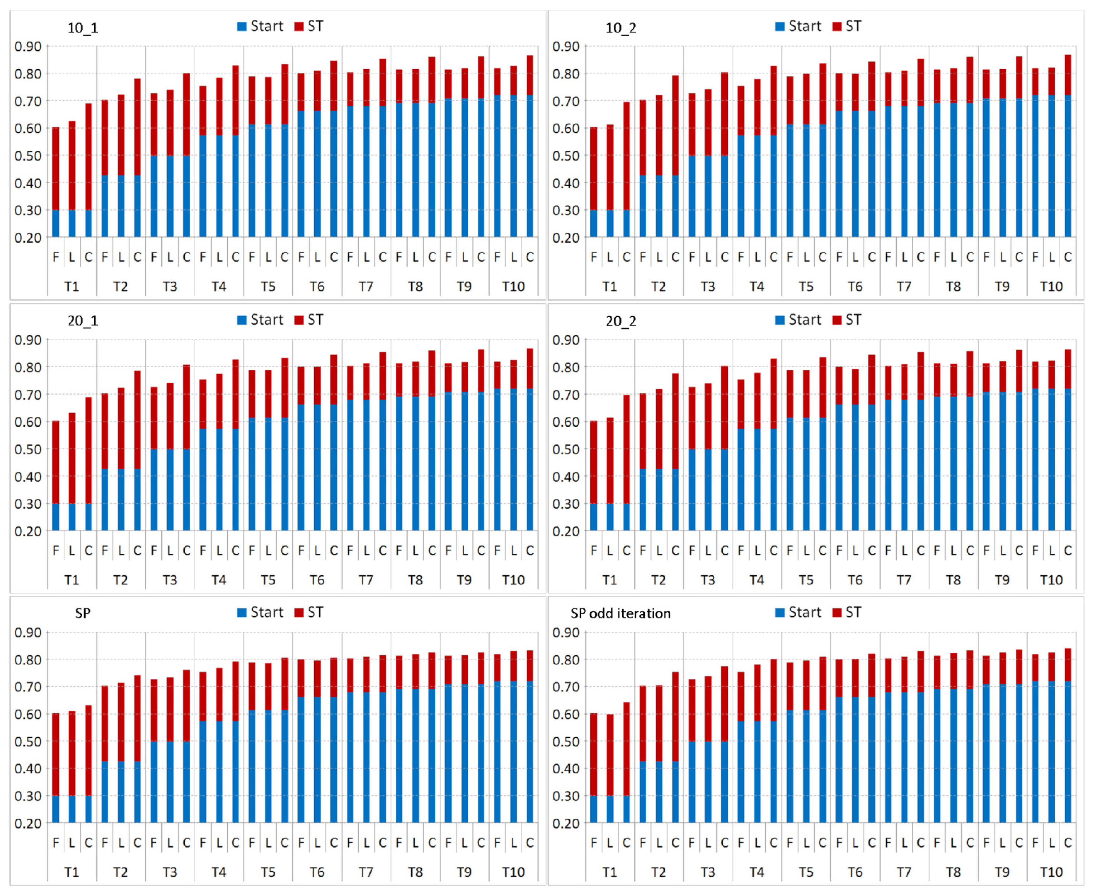
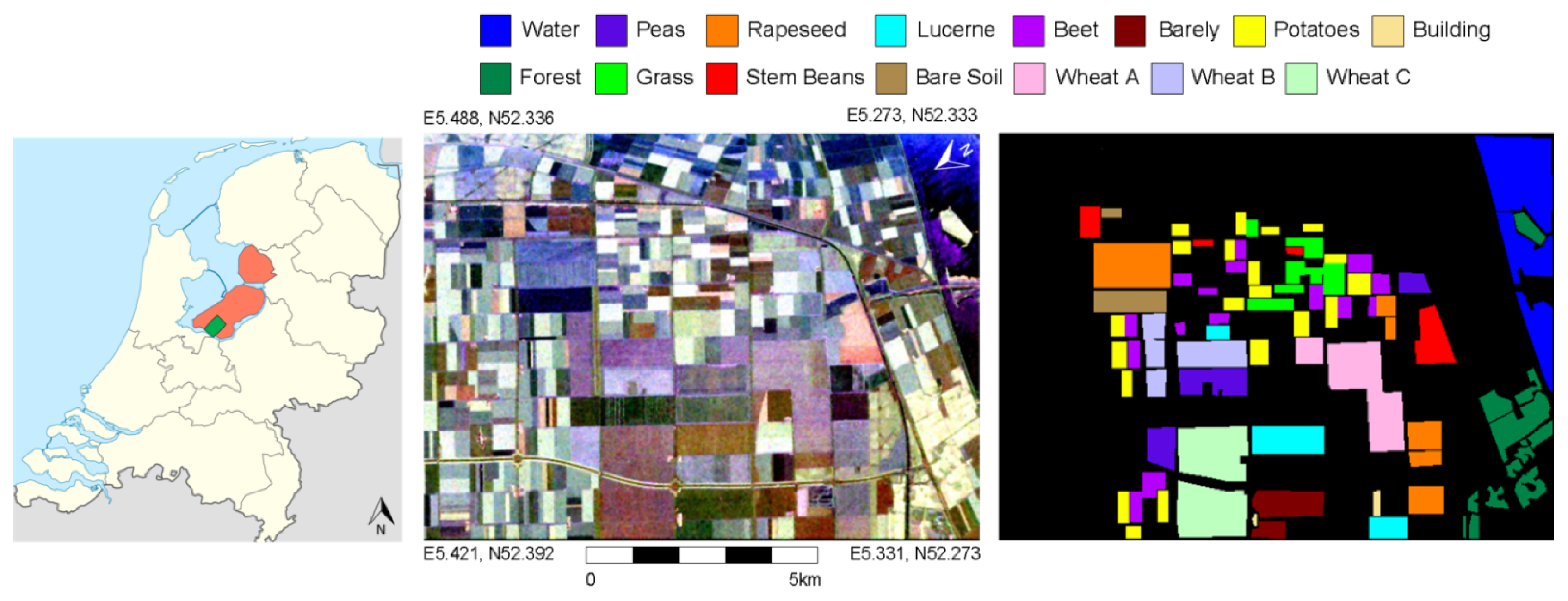
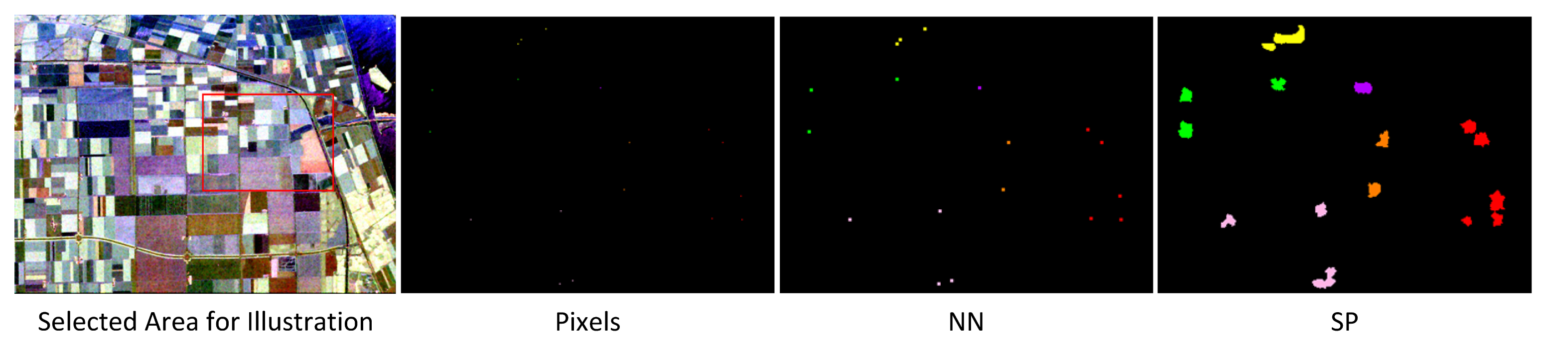
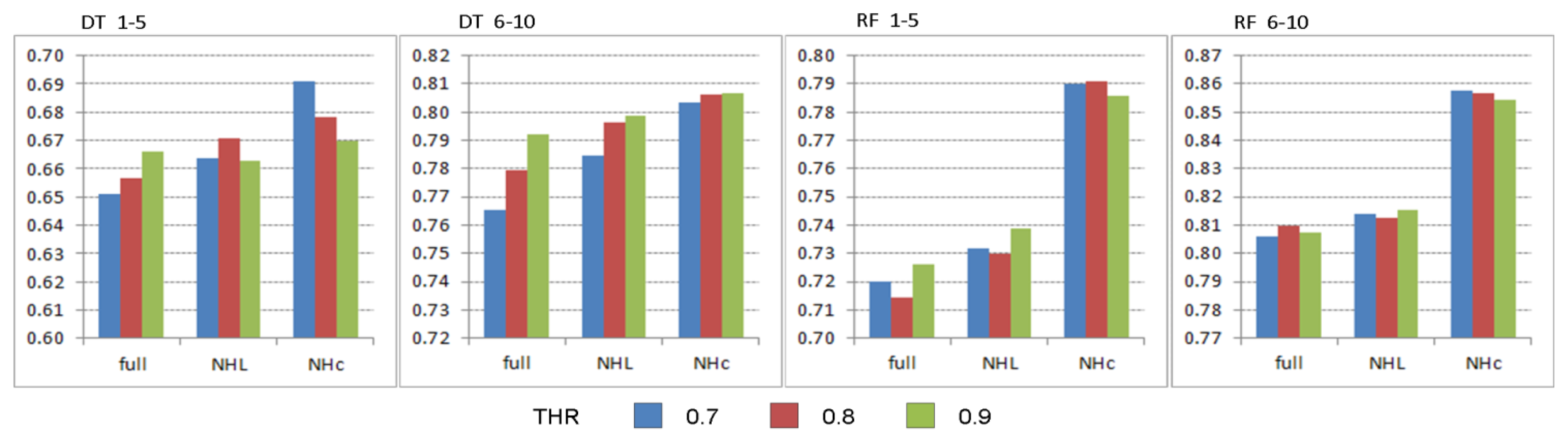
Before presenting the classification results over the initial training sets, T_i, using self-training with the ensemble-based bagging approach, we shall first investigate the effects of the confidence threshold, the different proposed search neighborhoods, and the number of unlabeled samples selected. Furthermore, we shall evaluate and compare the performances of the enlarged training sets via the unsupervised SSL approaches, NN, and superpixels, SP. Along with the numerical performance evaluations represented as average classification accuracies over the 10 instance for the different training sets size T_i; we shall also present visual classification results.

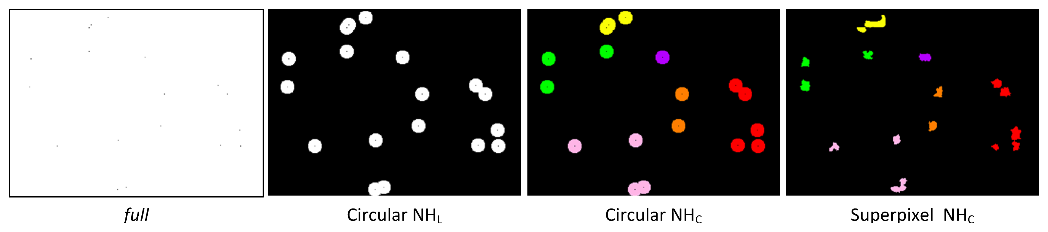
For evaluation of the effects with respect to the confidence threshold THR, we used a basic setup using the three search neighborhoods, full, circular NH_L, and circular NH_c using DT and RF within the ensemble based self- training. We considered three values for THR: 0.7, 0.8, and 0.9. Individual results are shown in Figure 7 as average classification accuracies achieved over the smaller and larger sized training sets. Using RF, the different THRs perform on a similar level and differences among search neighborhoods with minor variations in the final classification accuracies, due to being a stronger classifier providing better class predictions over smaller training sets. However, the weaker classifier DT is more affected by the choice of THR as one probably would expect. The main observation is that the THR has an effect on the final classification performance with respect to the underlying search neighborhood. The DT performance regarding THR seems to be proportional to the size of the used search neighborhood. With a smaller THR is seems beneficial to have a smaller search neighborhood, whereas with higher THR the size of the search neighborhood does not seem to have major effects as performances vary just within a small margin. This is expected as the weaker learner DT is not able to learn and generalize too well from such tiny to small training sets. Due to these observations and as the overall classification performances for the different THRs average out over the different search neighborhoods, we consider THR = 0.8 for the remainder of our experiments over both base learners.

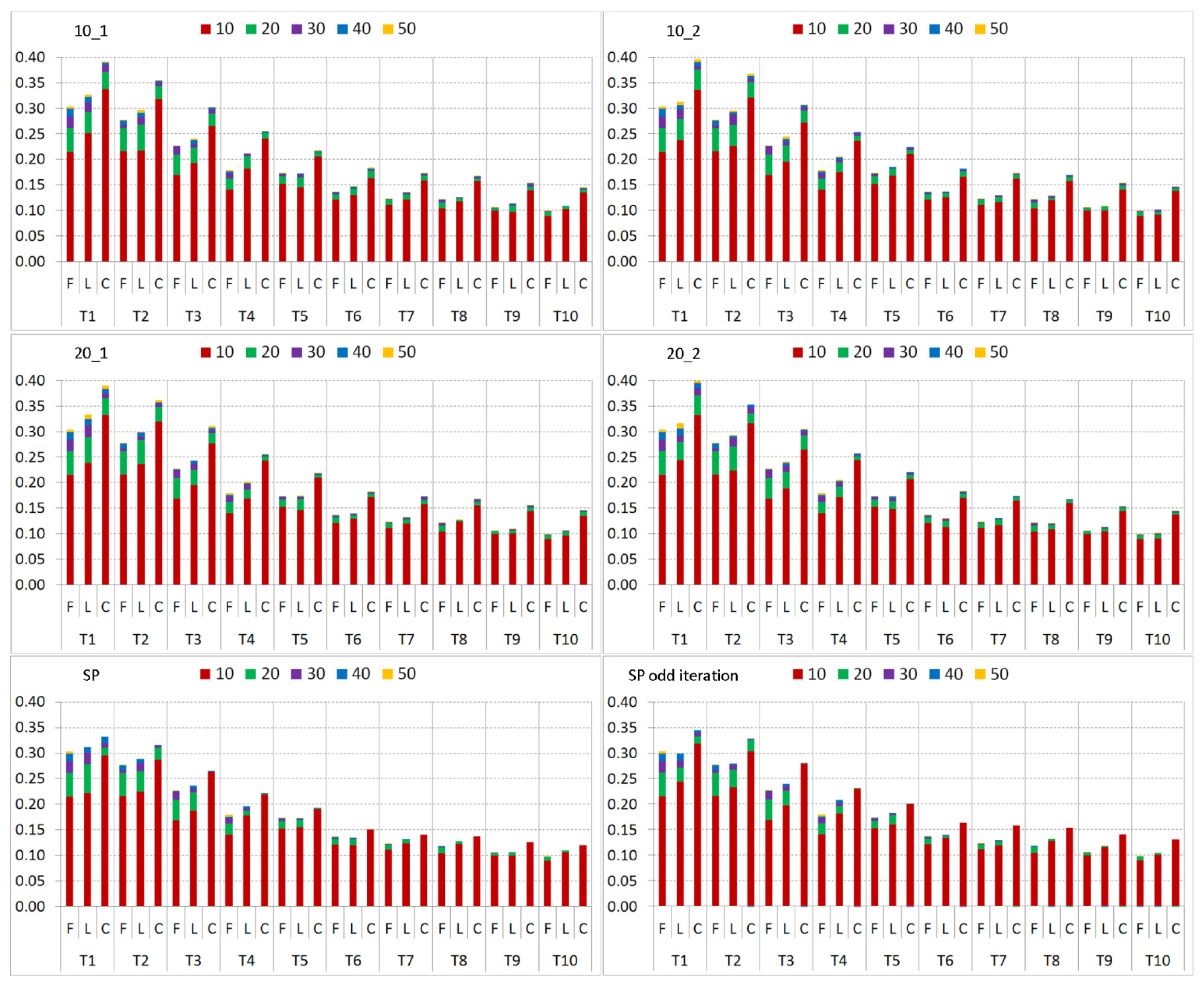
Regarding the evaluation of the different search neighborhoods (SNHs), the overall differences in total gain after 50 iterations of ST is minimal with all SNHs reaching similar classification results (Figure 8) and ST improvements (Figure 9) for different T_i. We can see that especially with the small T_i (T₁–T₅) larger ST improvements can be obtained compared to their initial lower classification accuracies indicating that there is more potential for improvements. It is also anticipated that the ST improvements with the larger T_i (T₆–T₁₀) are no longer that significant (only around 10%–15%) as their initial classification accuracies are already around 60%–70% due to larger training data. In general, differences among the SNHs full, NH_L, and NH_C are observed as expected. Applying NH_L results in slightly better results than using full since NH_L is a smaller subset of full whereas NH_C limits the SNH for one class to the spatial proximity of its particular labeled samples. The performance difference between full and NH_L disappears for the larger sets, T_5–10, since NH_L suffers from the same problem, i.e., no or limited amount of new information is available due to larger number of labeled samples.

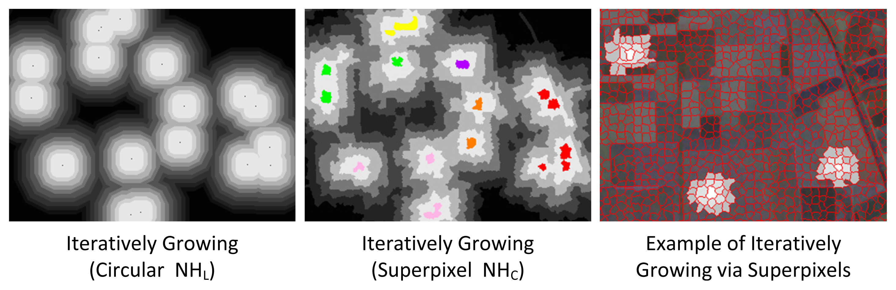
For the circular NH_L and NH_C, the initial size rad and the incremental expansion by radInc seems to have marginal effects since in either case the SNH area will not significantly change with each iteration. Overall, the four different combinations result in rather similar outcomes with marginal variations due to the random sample selection. Based on the observations, the influence of parameters rad and radInc are related to the SAR image resolution. Considering the two SP growing methods, in both cases results using NH_L are similar to full due to the fast rate the SP SNH grows. However, main differences can be observed for NH_C. Firstly, both methods results are below the ones obtained by circular growing, and in either case, no ST improvements for larger T_i are achieved after 10 iterations. Within the first 10 ST iterations, the best performance is achieved. Afterwards no further benefits of adding new samples can be made with NH_C since the SNH area is the same size as full.

For the main classification performance evaluations, we shall consider the NH_C approaches for the circular combination with rad = 10 and radInc = 1. This mimics the slower growth while the superpixel approach will much faster while expanding the SNH every odd ST iteration. We shall abbreviate the two SNH approaches with NH_o for the circular and NH_sp for the superpixel methods.

Next, we shall investigate the effect of the number of unlabeled samples that are added per ST iteration. Due to small sample number per class, we only consider the same amount of unlabeled samples as labeled per class for initial pixel training sets T_i. Thus, for enlarging T_i with NN and SP, we evaluated the effect of adding different number of unlabeled samples per ST iteration. For this, we consider multiples (xL) of labeled samples per class, namely x1, x2, x4, and x6. This means, for example, that in case of x4, unlabeled data size is up to 4 times of the size of labeled samples that they can be added per class. Thus with i = 2, this results in 8 possible candidates if their confidence scores are higher than THR. Based on our previous observations, we shall consider NH_o and NH_sp, in particular.

Figure 10 demonstrates the differences of several search neighborhoods (SNHs) and number of xL combinations with respect to the best classification result achieved among all combinations. The general observation confirms the expected result, that is, adding more unlabeled samples than the initially labeled samples will bias the learning process towards the unlabeled samples particularly in case of the smaller training sets, i.e., T_1–5, as shown in the plot for Decision Tree (DT) over NN_i using SNH mode, full. However, this effect is reduced for T_6–10 due to the relatively larger size of the initial training data. When using NH_sp, it shows the same behavior for different xL combinations as it will reach the area of full since the search process quickly suffers from the same issues. Yet note that the effects are not as severe since the SNH still has to grow within the first ST iterations, which reduces the chance of the weak DT learner to add erroneous samples during the first ST iterations. Applying NH_o appears to provide best results among all combinations with x4 combination being a trade-off to x2 and x6 combinations as a balance between the number of labeled and unlabeled samples. Yet classification accuracy differences among them are rather small, i.e., only within 1%. For the larger training sets of NN_6–10 using NH_o, there seems to be no benefit of adding more unlabeled samples due to larger number of labeled samples that are already available and providing initial classification accuracy level higher than 70%. In that regard, performance differences for x4 and x6 to x1 and x2 combinations are negligible. Concerning the superpixel enlarged initial training sets, results using SNHs, full and NH_sp seem to follow similar behavior for different xL combinations. However, classification accuracies are achieved within a 1% range due to the larger training set sizes and this makes it easier to compensate for larger number of unlabeled samples. In case of SP_i, the number of unlabeled samples does not significantly affect the final results, as the labeled data size during the initial training iterations is so large that only minor ST improvements can be made.

Regarding the evaluation using Random Forest (RF), we can observe similar behavior for the different training sizes. As for DT with NN_i using the SNH mode as full, more unlabeled samples result in higher probabilities of selecting erroneous samples due to the larger SNH. For NH_sp, due to the homogeneous superpixels, the size of unlabeled samples has a marginal effect because the additional samples over the same superpixel area will have a rather similar feature structure especially with a stronger classifier that is capable of providing higher confidence scores. Nonetheless, we can observe that for NH_o the opposite effect is visible, where more samples can now make a significant influence. One of the reasons is that the circular NH grows with respect to the spatial distance to a labeled sample location—not as in case of superpixels by sample homogeneity. More important than this is the fact that with NH_o the SNH grows slower so that not all similar samples are added within the same ST iteration. The addition of similar samples is spread over time and many ST iterations For the enlargement of T_i by superpixels as for DT, similar observations can be made for NN_6–10 and SP, where the effect of the unlabeled samples is reduced with higher number of labeled samples.

The initial classification performances of T_i and their corresponding self-training (ST) improvements for search neighborhoods full, NH_o, and NH_sp are shown in Figure 11. In our setup using DT as the base classifier, we can observe that similar level of classification accuracies can be achieved using self-training over T₁, T₂, and T₃ compared to the initial results of T₄, T₇, and T₁₀, respectively. Similarly, when employing RF with the sets T₁ and T₂ using self-training, classification results comparable to T₅ and T₁₀ can be realized. This is not surprising because the stronger base classifier such as RF can achieve higher classification accuracies particularly for small training sets such as T₁ and T₂, and this results in better label predictions of the unlabeled samples in the first ST iterations. Note that for both base classifiers, the classification accuracy level that is achieved by self-training while using initially 3–5 times less amount of manually labeled data, is similar to the one obtained with its SL counterpart. Such a crucial reduction on the manually labeled data for training is indeed a noteworthy accomplishment of the ST approach; however, we shall carry out further investigations to evaluate different options and to maximize the gain.

We illustrate the effect of the 10 different training set instances of T₁ and T₂ in Figure 12. The plots show that for instances of T₁ and T₂ DT are struggling with the small number of labeled samples to achieve improvements via ST. As mentioned earlier, the initial labeled samples are critical to determine the success of applying SSL particularly for such a weaker learner as DT. It can be noticed that using RF (as a mini-ensemble of three DTs) is overcoming this problem and significant improvements are achieved within the first 10 ST iterations. Furthermore, as T₁ is a subset of T₂, it can be seen that the one additional sample per class has a positive influence yet will not always overcome the weakness of the first sample or might even have a negative effect.

Evaluating the three different methods on “how” and “where” to pick the unlabeled samples from, we can observe clear differences for the two base classifiers employed. For the weaker classifier, DT, the full search neighborhood provides slightly better or similar results than NH_o and NH_sp for T₁ and T₂, whereas for the larger sets T_3–10, NH_o and NH_sp yield higher accuracies. The reason lies in the fact that DT, as a rather weak learner is not capable of learning from such small sample sizes with one and two labeled samples per class. For T₁, note that DT still benefits from new samples during the iterations, t = 40 and t = 50. However, note that ST improvements of 18%–22% are achieved due to the extremely low initial classification accuracies on the labeled samples while the overall classification accuracies being below 50%. As for the larger sets, T_3–10, the larger training data size in a greater search neighborhood while increasing the number of possible unlabeled candidates within NH_o and NH_sp. Yet the number of these candidates is still significantly smaller than the one for full and this yields a higher chance to semi-labeled samples with lower class confidence values providing more diversity but in the same time, higher risk of erroneous semi-labeling. However, performance differences observed among different search neighborhoods are minimal, i.e., using NH_o provides a mere ~2% higher classification accuracies. As for RF, classification performances over T_1–4 using NH_o are the highest among all other alternatives. This is related to the stronger classifier that has a superior learning capabilities with less number of samples so that the smaller search neighborhood of NH_o and NH_sp becomes then quite beneficial in providing more diverse samples into the learning process. Both base classifiers indeed benefit from selecting samples closer to the initially labeled samples while having a stronger classifier with a better learning ability is obviously more advantageous.

Furthermore, when looking into the self-training iterations in Figure 11, we can observe that using NH_o and NH_sp can yield further improvements particularly during the earlier iterations (i.e., t = 10). With the full search neighborhood, either a minimum number of 20–30 iterations are needed to achieve the same results or for a larger T_i, similar accuracies cannot be achieved even after 50 iterations when using DT as the base classifier. The same behavior can also be observed for RF, where results obtained after 10 iterations applying NH_o and NH_sp outperform accuracies achieved after 50 iterations applying full as the search neighborhood. Note further that performing self-training over these initial training sets achieves similar or better results than using NN_i or SP_i, respectively. This is due to the fact that the neighborhood, full, can result in larger numbers of unlabeled samples with high classifier confidence scores that are greater than THR. Hence, there is a greater chance for the highly accurate semi-labeled samples to be selected; however, this yields adding no or less new information into the self-training process. In case of NH_o and NH_sp, the number of possible unlabeled samples as new candidates is limited, therefore, giving a higher chance of adding more diversity due to the samples with a lower confidence score. When using NH_sp, the best performance is achieved within the first 10 iterations, after that its SNH area grows beyond full. Since the classification accuracy with NH_sp after 10 iterations is already better than the one achieved with full using 50 iterations, no further benefits of adding new samples can be observed with NH_sp.

When enlarging T_i to NN_i, the initial classification performance is improved as illustrated in Figure 13, which is anticipated due to the availability of more samples. As we have the ground truth available, we could verify that 96.3% of the NN_i samples are correctly labeled whereas the majority of the remaining 3.7% is unknown since no ground truth is available on those sections. Even though, it is expected that NN₁ and T₉ results are not comparable because the NN₁ samples will have a similar feature structure providing less diversity among the samples compared to the nine labeled samples in T₉. This is also observable for the NN_2–4 results as they are not able to match the initial classification accuracy of T₁₀ besides NN_2–4 being significantly larger.

The initial classification improvements on the average are ~18% and ~10% for NN_1–5 and NN_6–10, respectively. Note that employing self-training is still able to provide an increase in the classification accuracy over all NN_i yet the improvements are getting insignificant, as the initial accuracies are higher (see Figure 13). At the end, this results in classification performance employing NH_o/NH_sp being just marginally better by 0.5% for DT and ~2.5% for RF, on the average than using full.

When DT is used as the base classifier, the main performance difference compared to the results with T_i is that NN_i is highly beneficial for labeled dataset size of i = 2 when improving the final classification accuracy by 6%–7%. Similar observation can be made for RF trained over the NN₁ where an accuracy improvement of around 6% is visible for the search neighborhood full compared to their T₁ results. However, employing NH_o and NH_sp over both training sets T₁ and NN₁, the difference shrinks to 2%. For training sets larger than T_3, the performance difference between the application of T_i and NN_i is minimal. The reason for this is that both NN_i and NH_o/NH_sp enhance the initial training set T_i based on the same idea: by selecting unlabeled samples from the close neighborhood of the provided labeled samples.

Similar observations and comparative evaluations between the superpixel method and NN_i can be made. As visible in the plot given in Figure 14, compared to NN₁, the classification accuracy over the SP₁ can be improved by 15% and 11% for DT and RF, respectively, whereas performance differences for the other training set sizes are getting less. Similar to NN_i, such improvements occur as a result of significantly larger dataset size for self-training, i.e., around 100 semi-labelings per labeled pixel. However, when verified with the ground truth, we can note that the accuracy of the correctly labeled superpixel samples using superpixel method is lower than the one for NN (around 10%), yet there are still at least 86 of 100 samples with the correct labels whereas the other 14% are mainly unknown. It is obvious that the relative drop in the semi-labeling accuracy is compensated by the significantly larger number of samples providing more diversity. Moreover, the superpixel method already covers most potential candidates within the vicinity of the initially labeled samples and thus reduces the effect of NH_o and NH_sp. When the search strategies full is employed the amount of new information is quite limited and note that it is now further reduced due to the larger diversity already introduced by the larger training data. Hence, this significantly reduces any potential performance gain. The same effect can also be observed for the larger T_i or NN_i training sets. This means that an upper bound of classification accuracy can be achieved by employing different sized training sets.

Over both neighborhood approaches NN_i and SP_i of the proposed self-training method, we perform comparative evaluations among the three training set types. Figure 15 presents the plots that sum up the differences of the classification accuracies obtained by individual NN_i and SP_i approaches with respect to their initial training set, T_i. When using DT as the base classifier, the neighborhood superpixel approach contributes by at least 5% to the classification accuracy for the most of the training sample sizes used whereas the highest gain is achieved when the two smallest training sets are enlarged by their 8-connected neighbors. When using RF as the base classifier, improvements are observed for all sets over the search neighborhood full where accuracy differences over NN_i and SP_i are around +2% and +6%, respectively. We observe that when exploiting the closer spatial neighborhood of labeled samples via NH_o, neither the 8-neighbor contextual information approach nor the superpixels approach leads to any significant performance improvement due to the aforementioned reasons.

Along with the numerical evaluations, we shall further present visual classification results, from the initial to the final classification output. Figure 16 illustrates the sample classification maps using RF as the base classifier within the ensemble-based bagging approach. In the figure, we also visually compare the effects of search neighborhoods, full and NH_o, over the classification performance and the top row shows the initial results over an instance of T₂. The images displaying the “difference to ground truth” show the major misclassification of a particular class while white indicating correct labels. Thus, larger white areas represent a better match with the ground truth. The green circles for the classification results annotated with the ST iteration number 10 in row 2 indicate the classification difference between the two search neighborhoods, full and NH_o, compared to the initial results from the labeled samples in the first row. In particular, this row shows the difference between the classification performances achieved using two neighborhood approaches, NH_o and full both visually and numerically. For the following rows, the green and red circles indicate higher improvements or degradations, respectively, compared to the corresponding previous row. Overall, it is clear from the figure that major improvements after 10 iterations are achieved by applying NH_o and during the rest of the 20 iterations, only minor improvements are observed. As visible in the final numerical classification results, the application of the other neighborhood approach, full, yields an improvement for the major areas after 20 iterations, yet does not achieve better results.

For visual and numerical comparisons of the different SSL approaches, Figure 17 shows results for the initial T_i, NN_i, SP_i, T_i in self-training, and initial T₁₀ training sets. The first four are based on an instance of T₂ while T₁₀ is chosen based on the numerical results for RF. It is worth noting that the visual classification results achieved by RF with SL over the set T₁₀ and with SSL by self-training over T₂ applying NH_o are quite similar. The green circles mark the best classification performance in a particular area among all classification results. The comparison shows that the classification over T₂ with the application of SSL employing NH_o produces the best classification map.

This is a significant accomplishment achieved by SSL along with a classifier initially trained with a small-sized training dataset particularly when comparing to the classifier trained over the set T₁₀ and thus having 5 times more user-labeled samples to form the training dataset. In this example, the visual results favor NN₂ to SP₂; however, this is vice versa when numerical results are compared. This is related to the particular T₂ instance and the corresponding superpixels. This shows that the starting point can be particularly critical for SSL especially when small sample sized training sets are used for the initial training.

Finally, we shall provide a brief comparison among various classifiers. They have been evaluated over different training set sizes such as 52, 104, 208, and 1041 samples, which correspond to 0.25‰, 0.5‰, 1%, and 5% of the 208 000 pixel ground truth, respectively. All classifier parameters have been optimized for the best classification performance; and their classification accuracies are averaged over 100 runs using HαA features and shown in

Table 1. Results over the covariance matrix 〈[C]〉 and HαA features with various supervised classifiers.

	DT		ELM		MLP		KNN
	〈[C]〉	HαA	〈[C]〉	HαA	〈[C]〉	HαA	〈[C]〉	HαA
52	0.42	0.55	0.31	0.62	0.23	0.57	0.48	0.66
104	0.53	0.66	0.53	0.71	0.28	0.67	0.54	0.73
208	0.60	0.73	0.63	0.78	0.35	0.75	0.59	0.77
1041	0.68	0.82	0.75	0.86	0.50	0.88	0.69	0.86

Table 1. Results over the covariance matrix 〈[C]〉 and HαA features with various supervised classifiers.

	RF		SVM (Linear)		SVM (Polynomial)		SVM (rbf)
52	0.63	0.78	0.54	0.72	0.53	0.71	0.54	0.72
104	0.70	0.83	0.63	0.79	0.61	0.79	0.62	0.80
208	0.75	0.86	0.70	0.84	0.68	0.83	0.67	0.85
1041	0.81	0.90	0.80	0.90	0.75	0.90	0.75	0.91

. Details about the optimization process and setup for the supervised classifiers can be found in [41]. As an additional comparison, we also added the classification results using the covariance matrix 〈[C]〉 to Table 1 besides the HαA feature results.

Our previous experiments and evaluations have shown that SSL and ST using small-labeled data are able to achieve similar classification performances compared to supervised learning with larger labeled data sets using the same underlying classifier. The same observation can be made for typical classifiers such as KNN, MLP, and SVMs as illustrated in Figure 18. The most interesting fact is that training sets with 6 or more samples per class using superpixels to enlarge the initial labeled data combined with the ensemble-based self-training is able to achieve comparable classification performances with various SL methods using as high as 1000 labeled samples.

5. Conclusions

In this paper, we have investigated different approaches of semi-supervised learning over polarimetric SAR data while the focus is on the small sample size problem. Unsupervised methods such as contextual information (i.e., connected neighbors) or clustering/segmentation approaches (i.e., superpixels) to enlarge the initial labeled training set have shown promising results to address the small sample size problem in the right direction. Additionally, the employed self-training approach using an ensemble-based approach has proven beneficial especially in cases when it can achieve similar classification results over small training sets compared to the classification results of the classifiers trained over significantly larger training sets.

Furthermore, we have principally shown that different strategies on how to select reliable candidates from a large set of unlabeled samples can speed-up and improve the classification performance. In particular, for a remote sensing application such as polarimetric SAR image classification, it is advantageous to exploit the location-based information from the labeled training data. The choice of the applied confidence threshold can be critical particularly for weaker classifiers, where an adaptive approach can be applied starting with larger values and slowly decreasing it over time. However, we have also shown that this approach alone cannot guarantee to achieve such a classification performance that is beyond a certain level since the initial labeled set size is critical particularly when it is small. Nevertheless, in accordance with the number of base classifiers in the ensemble approach, it will still help to decrease the number of semi-supervised learning iterations by achieving similar or even better results.

We can foresee that there is an imminent need to investigate different strategies further in order to reliably and in a most informative way select unlabeled samples, as well as to consider semi-supervised learning within the application of domain adaptation. These will be the topics for our future work.