Automated Detection of Cloud and Cloud Shadow in Single-Date Landsat Imagery Using Neural Networks and Spatial Post-Processing

Abstract
:1. Introduction
2. Background
3. Methods
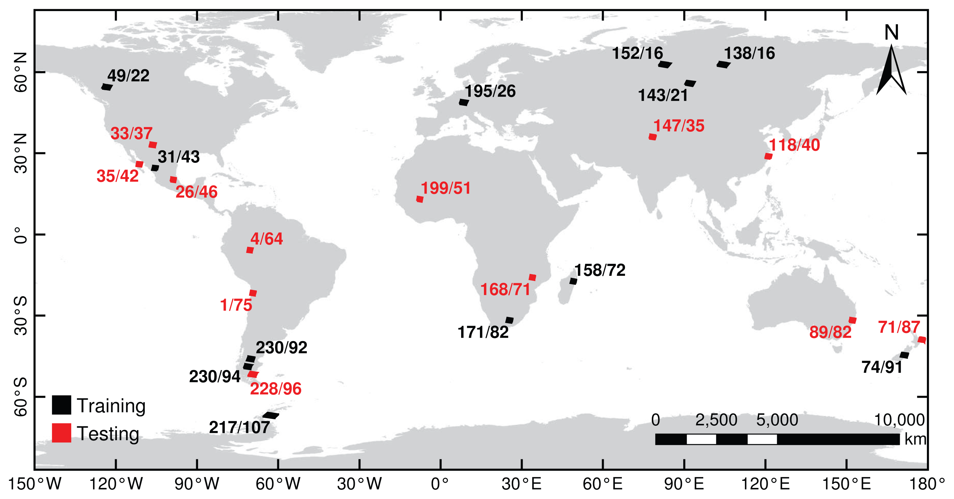
3.1. Data Sets
3.2. Neural Network Classification
3.3. Spatial Post-Processing
3.4. Classifier Assessment
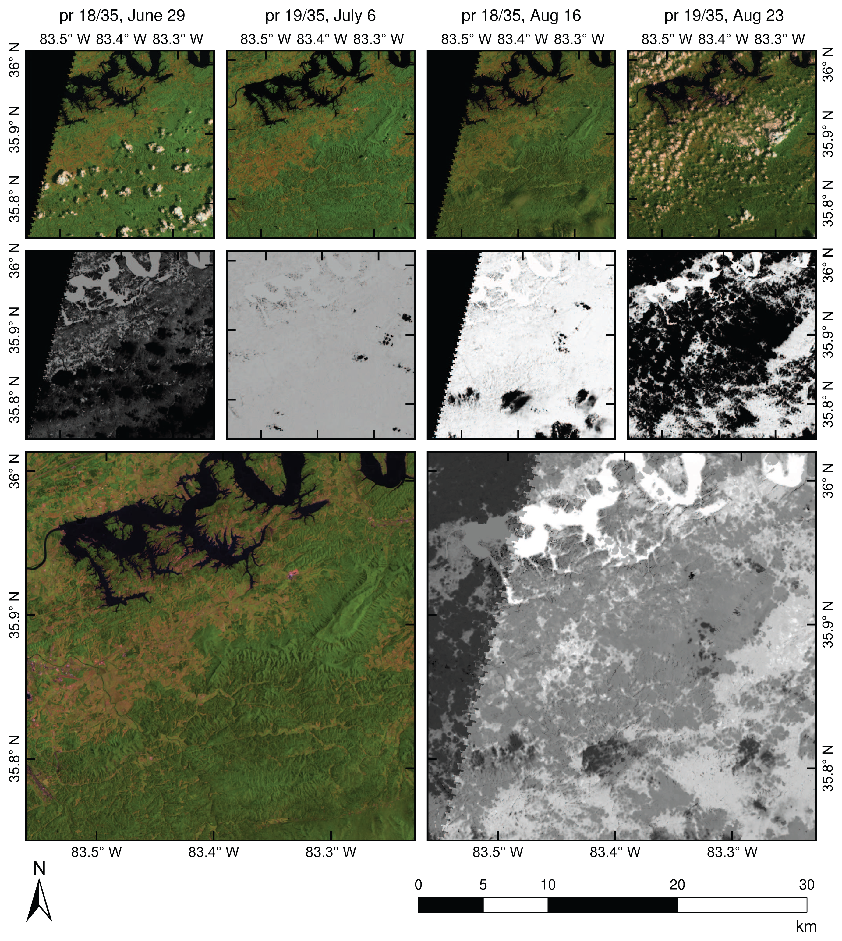
3.5. Application: Obstruction-Free Summertime Composites
4. Results and Discussion
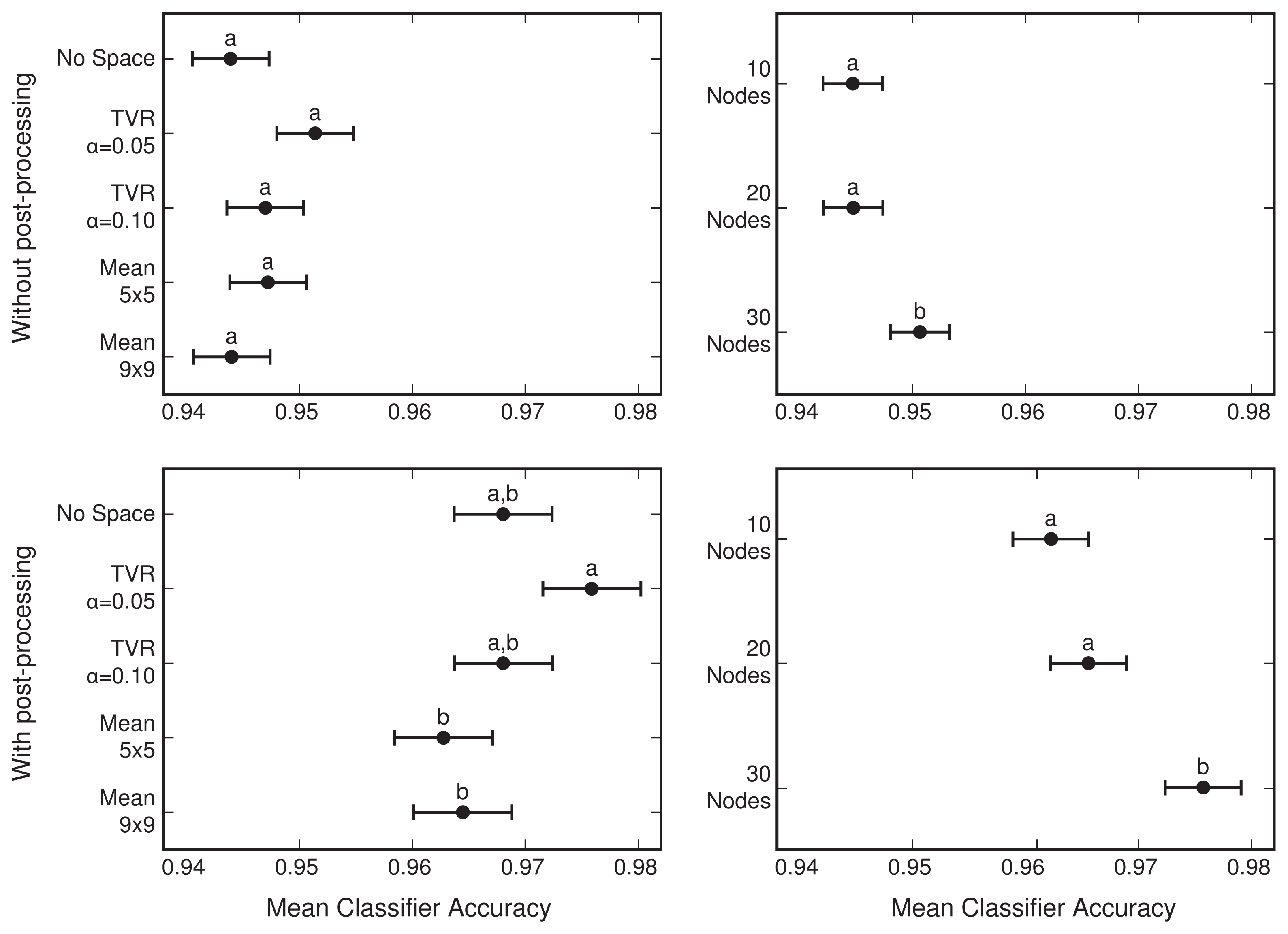
4.1. Network Selection
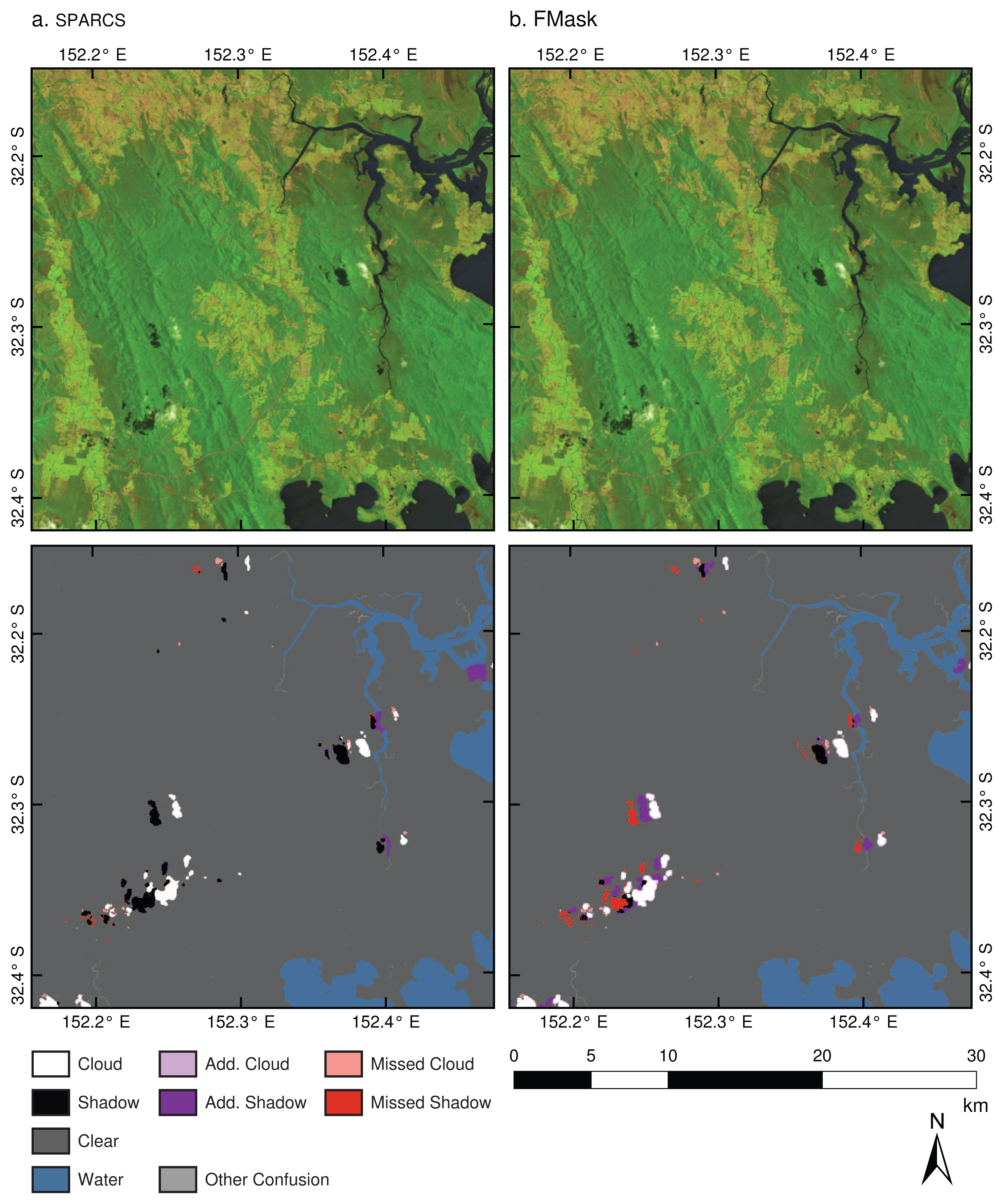
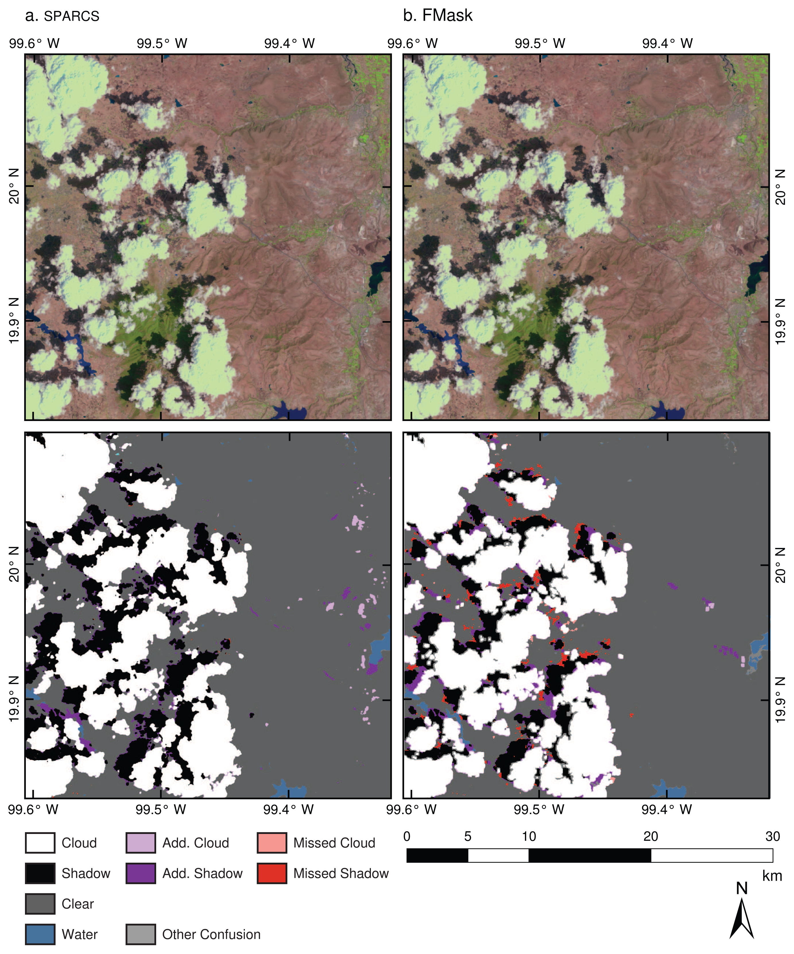
4.2. Comparison to FMask
4.3. Creating a Multi-Temporal Composite
5. Conclusions
Acknowledgments
Conflicts of Interest
- Author ContributionsJoseph Hughes developed methods, created the evaluation dataset, and analyzed results. Daniel Hayes supervised research. Joseph Hughes and Daniel Hayes wrote the manuscript.
References
- Ju, J.; Roy, D.P. The availability of cloud-free Landsat ETM+ data over the conterminous United States and globally. Remote Sens. Environ 2008, 112, 1196–1211. [Google Scholar]
- Saunders, R.; Kriebel, K. An improved method for detecting clear sky and cloudy radiances from AVHRR data. Int. J. Remote Sens 1988, 9, 123–150. [Google Scholar]
- Derrien, M.; Farki, B.; Harang, L. Automatic cloud detection applied to NOAA-11/AVHRR imagery. Remote Sens. Environ 1993, 46, 246–267. [Google Scholar]
- Cihlar, J.; Howarth, J. Detection and removal of cloud contamination from AVHRR images. IEEE Trans. Geosci. Remote Sens 1994, 32, 583–589. [Google Scholar]
- Simpson, J.; Stitt, J. A procedure for the detection and removal of cloud shadow from AVHRR data over land. IEEE Trans. Geosci. Remote Sens 1998, 36, 880–890. [Google Scholar]
- Ackerman, S.A.; Strabala, K.I.; Menzel, W.P.; Frey, R.A.; Moeller, C.C.; Gumley, L.E. Discriminating clear sky from clouds with MODIS. J. Geophys. Res 1998, 103, 32141–32157. [Google Scholar]
- Gao, B.; Kaufman, Y. Selection of the 1.375-μ m MODIS channel for remote sensing of cirrus clouds and stratospheric aerosols from space. J. Atmos. Sci 1995, 52, 4231–4237. [Google Scholar]
- Luo, Y.; Trishchenko, A.; Khlopenkov, K. Developing clear-sky, cloud and cloud shadow mask for producing clear-sky composites at 250-meter spatial resolution for the seven MODIS land bands over Canada and North America. Remote Sens. Environ 2008, 112, 4167–4185. [Google Scholar]
- Oreopoulos, L.; Wilson, M.J.; Várnai, T. Implementation on Landsat data of a simple cloud-mask algorithm developed for MODIS land bands. IEEE Geosci. Remote Sens. Lett 2011, 8, 597–601. [Google Scholar]
- Martinuzzi, S.; Gould, W.; González, O. Creating Cloud-Free Landsat ETM+ Data Sets in Tropical Landscapes: Cloud and Cloud-Shadow Removal; General Technical Report IITF-GTR-32; International Institute of Tropical Forestry: Ro Piedras, Puerto Rico, 2007; pp. 1–18. [Google Scholar]
- Choi, H.; Bindschadler, R. Cloud detection in Landsat imagery of ice sheets using shadow matching technique and automatic normalized difference snow index threshold value decision. Remote Sens. Environ 2004, 91, 237–242. [Google Scholar]
- Hollingsworth, B.; Chen, L.; Reichenbach, S.E.; Irish, R.R. Automated cloud cover assessment for Landsat TM images. Proc. SPIE 1996, 2819, 170–179. [Google Scholar]
- Goodwin, N.R.; Collett, L.J.; Denham, R.J.; Flood, N.; Tindall, D. Cloud and cloud shadow screening across Queensland, Australia: An automated method for Landsat TM/ETM+ time series. Remote Sens. Environ 2013, 134, 50–65. [Google Scholar]
- Kennedy, R.E.; Schroeder, T.A.; Cohen, W.B. Trajectory-based change detection for automated characterization of forest disturbance dynamics. Remote Sens. Environ 2007, 110, 370–386. [Google Scholar]
- Berendes, T.; Sengupta, S.; Welch, R.; Wielicki, B.; Navar, M. Cumulus cloud base height estimation from high spatial resolution Landsat data: A Hough transform approach. IEEE Trans. Geosci. Remote Sens 1992, 30, 430–443. [Google Scholar]
- Hagolle, O.; Huc, M.; Pascual, D.; Dedieu, G. A multi-temporal method for cloud detection, applied to FORMOSAT-2, VENS, LANDSAT and SENTINEL-2 images. Remote Sens. Environ 2010, 114, 1747–1755. [Google Scholar]
- Huang, C.; Thomas, N. Automated masking of cloud and cloud shadow for forest change analysis using Landsat images. Int. J. Remote Sens 2010, 31, 37–41. [Google Scholar]
- Zhu, Z.; Woodcock, C.E. Object-based cloud and cloud shadow detection in Landsat imagery. Remote Sens. Environ 2012, 118, 83–94. [Google Scholar]
- Haykin, S. Neural Networks and Learning Machines, 3rd Ed ed; Pearson Education Inc.: Upper Saddle River, NJ, USA, 2008. [Google Scholar]
- Scaramuzza, P.L.; Bouchard, M.A.; Dwyer, J.L. Development of the Landsat data continuity mission cloud-cover assessment algorithms. IEEE Trans. Geosci. Remote Sens 2012, 50, 1140–1154. [Google Scholar]
- Rudin, L.; Osher, S.; Fatemi, E. Nonlinear total variation based noise removal algorithms. Phys. D Nonlinear Phenom 1992, 60, 259–268. [Google Scholar]
- Goldstein, T.; Osher, S. The split bregman method for L1-regularized problems. SIAM J. Imaging Sci 2009, 2, 323–343. [Google Scholar]
- Hall, D.K.; Foster, J.L.; Verbyla, D.L.; Klein, A.G.; Benson, C.S. Assessment of snow-cover mapping accuracy in a variety of vegetation-cover densities in central Alaska. Remote Sens. Environ 1998, 137, 129–137. [Google Scholar]
- Crist, E.P. A TM tasseled cap equivalent transformation for reflectance factor data. Remote Sens. Environ 1985, 306, 301–306. [Google Scholar]
- MacQueen, J. Some Methods for Classification and Analysis of Multivariate Observations. Proceedings of the Fifth Berkeley Symposium on Mathematical Statistics and Probability, Berkeley, California, USA, 21 June–18 July 1967; University of California Press: Berkeley, CA, USA, 1967; 1, pp. 281–297. [Google Scholar]
- Moran, M.; Jackson, R.; Slater, P.; Teillet, P. Evaluation of simplified procedures for retrieval of land surface reflectance factors from satellite sensor output. Remote Sens. Environ 1992, 41, 169–184. [Google Scholar]
- Chander, G.; Markham, B.L.; Helder, D.L. Summary of current radiometric calibration coefficients for Landsat MSS, TM, ETM+, and EO-1 ALI sensors. Remote Sens. Environ 2009, 113, 893–903. [Google Scholar]
- Chavez, P.S. Image-based atmospheric corrections—Revisited and improved. Photogramm. Eng. Remote Sens 1996, 62, 1025–1036. [Google Scholar]
- Beale, M.H.; Hagan, M.T.; Demuth, H.B. Neural Network Toolbox User’s Guide, r2013b ed; The MathWorks, Inc: Natick, MA, USA, 2013. [Google Scholar]
- Zar, J.H. Biostatistical Analysis, 5th ed; Prentice-Hall: Upper Saddle River, NJ, USA, 2010. [Google Scholar]
- Kramer, C.Y. Extension of multiple range tests to group means with unequal numbers of replications. Biometrics 1956, 12, 307–310. [Google Scholar]
- Traver, V.J.; Bernardino, A. A review of log-polar imaging for visual perception in robotics. Robot. Auton. Syst 2010, 58, 378–398. [Google Scholar]


| # | Network Size (h) | Spatial Averaging Method (Calculated over Tassel-Cap) | Intensity of Spatial Averaging |
|---|---|---|---|
| 1 | 10 | No Space | - |
| 2 | 10 | Local Average | 5 × 5 Window |
| 3 | 10 | Local Average | 9 × 9 Window |
| 4 | 10 | TVR | α = 0.05 |
| 5 | 10 | TVR | α = 0.10 |
| 6 | 20 | No Space | - |
| 7 | 20 | Local Average | 5 × 5 Window |
| 8 | 20 | Local Average | 9 × 9 Window |
| 9 | 20 | TVR | α = 0.05 |
| 10 | 20 | TVR | α = 0.10 |
| 11 | 30 | No Space | - |
| 12 | 30 | Local Average | 5 × 5 Window |
| 13 | 30 | Local Average | 9 × 9 Window |
| 14 | 30 | TVR | α = 0.05 |
| 15 | 30 | TVR | α = 0.10 |
| Source | Sum Sq. | df | Mean Sq. | F | p |
|---|---|---|---|---|---|
| Type of Space | 0.004 | 4 | 0.001 | 1.51 | 0.198 |
| Network Size (h) | 0.004 | 2 | 0.002 | 3.18 | 0.043 |
| Sub-scene | 1.004 | 11 | 0.091 | 137.26 | <0.001 |
| Space×Size | 0.011 | 8 | 0.001 | 1.99 | 0.045 |
| Space×Sub-scene | 0.030 | 44 | 0.001 | 1.02 | 0.439 |
| Size×Sub-scene | 0.058 | 22 | 0.003 | 3.98 | <0.001 |
| Error | 0.298 | 448 | 0.001 | ||
| Total | 1.408 | 539 |
| Source | Sum Sq. | df | Mean Sq. | F | p |
|---|---|---|---|---|---|
| Type of Space | 0.011 | 4 | 0.003 | 2.53 | 0.040 |
| Network Size (h) | 0.018 | 2 | 0.009 | 8.17 | <0.001 |
| Sub-scene | 1.271 | 11 | 0.116 | 106.37 | <0.001 |
| Space×Size | 0.017 | 8 | 0.002 | 2.00 | 0.045 |
| Space×Sub-scene | 0.087 | 44 | 0.002 | 1.81 | 0.002 |
| Size×Sub-scene | 0.113 | 22 | 0.005 | 4.22 | <0.001 |
| Error | 0.487 | 448 | 0.001 | ||
| Total | 2.004 | 539 |
| Labeled as | Shadow | Cloud | Water | Snow/Ice | Clear |
|---|---|---|---|---|---|
| SPARCS | |||||
| Classed as Shadow | 94.7% | 1.0% | 2.3% | 1.7% | 0.5% |
| Cloud | 0.7% | 97.2% | 0.1% | 0.9% | 0.2% |
| Water | 0.5% | 0.0% | 96.6% | 1.0% | 0.1% |
| Snow/Ice | 0.9% | 0.4% | 0.0% | 90.2% | 0.0% |
| Clear | 3.2% | 1.3% | 1.0% | 6.2% | 99.2% |
| FMask | |||||
| Classed as Shadow | 69.9% | 0.5% | 0.6% | 7.6% | 2.4% |
| Cloud | 20.9% | 98.6% | 0.3% | 10.7% | 2.8% |
| Water | 1.0% | 0.0% | 96.6% | 0.0% | 0.0% |
| Snow/Ice | 0.3% | 0.0% | 0.0% | 72.4% | 0.1% |
| Clear | 8.0% | 0.9% | 2.4% | 9.3% | 94.7% |
| Missed Shadow | Missed Cloud | Over Shadow | Over Cloud | Overall | |
|---|---|---|---|---|---|
| Jammu and Kashmir, India: pr 147/35 (36.4°N, 78.8°E). 20 February 2001. | |||||
| SPARCS | 19.2% | 10.1% | 1.0% | 0.6% | 97.2% |
| FMask | 6.9% | 2.5% | 7.2% | 7.2% | 86.8% |
| New Mexico, USA: pr 33/37 (33.5°N, 105.9°W). 11 February 2001. | |||||
| SPARCS | 2.9% | 0.2% | 0.1% | 0.0% | 99.6% |
| FMask | 3.4% | 0.0% | 4.7% | 4.4% | 92.4% |
| Zhejiang, China: pr 118/40 (28.6°N, 120.4°E). 11 March 2001. | |||||
| SPARCS | 0.4% | 0.1% | 0.7% | 0.2% | 99.4% |
| FMask | 5.0% | 0.3% | 3.3% | 4.2% | 94.9% |
| Baja California Sur, Mexico: pr 35/42 (25.5°N, 111.1°W). 22 March 2001. | |||||
| SPARCS | 2.5% | 0.0% | 0.2% | 0.0% | 99.8% |
| FMask | 17.1% | 0.4% | 0.2% | 0.2% | 99.2% |
| Hidalgo, Mexico: pr 26/46 (20.0°N, 99.5°W). 1 February 2001. | |||||
| SPARCS | 0.2% | 0.0% | 1.0% | 0.7% | 98.9% |
| FMask | 9.1% | 0.5% | 2.1% | 0.5% | 97.4% |
| Koulikoro, Mali: pr 199/51 (13.3°N, 7.3°W). 30 January 2001. | |||||
| SPARCS | 0.0% | 0.0% | 0.0% | 0.0% | 100.0% |
| FMask | 0.0% | 0.0% | 0.6% | 0.3% | 99.1% |
| Amazon, Brazil: pr 4/64 (5.2°S, 70.9°W). 13 March 2001. | |||||
| SPARCS | 9.5% | 1.9% | 2.2% | 0.8% | 97.6% |
| FMask | 9.4% | 1.3% | 8.4% | 1.0% | 97.9% |
| Tete, Mozambique: pr 168/71 (16.2°S, 33.3°E). 10 April 2001. | |||||
| SPARCS | 0.0% | 0.0% | 0.0% | 0.0% | 100.0% |
| FMask | 0.0% | 0.0% | 0.0% | 0.0% | 100.0% |
| Antofagasta, Chile: pr 1/75 (21.4°S, 68.9°W). 20 January 2001. | |||||
| SPARCS | 17.7% | 18.0% | 2.5% | 0.0% | 96.4% |
| FMask | 24.8% | 7.4% | 7.2% | 13.5% | 79.8% |
| New South Wales, Australia: pr 89/82 (32.3°S, 152.3°E). 21 April 2001. | |||||
| SPARCS | 6.9% | 11.2% | 0.2% | 0.0% | 99.6% |
| FMask | 59.3% | 9.7% | 0.5% | 0.1% | 98.9% |
| Hawke’s Bay, New Zealand: pr 71/87 (39.2°S, 177.1°E). 12 April 2001. | |||||
| SPARCS | 9.1% | 0.8% | 1.1% | 0.2% | 98.6% |
| FMask | 12.7% | 2.1% | 0.1% | 0.1% | 99.8% |
| Santa Cruz, Argentina: pr 228/96 (51.9°S, 70.5°W). 11 January 2001. | |||||
| SPARCS | 3.9% | 1.4% | 1.0% | 2.5% | 97.8% |
| FMask | 6.8% | 0.4% | 5.0% | 2.5% | 97.1% |
© 2014 by the authors; licensee MDPI, Basel, Switzerland This article is an open access article distributed under the terms and conditions of the Creative Commons Attribution license (http://creativecommons.org/licenses/by/3.0/).
Share and Cite
Hughes, M.J.; Hayes, D.J. Automated Detection of Cloud and Cloud Shadow in Single-Date Landsat Imagery Using Neural Networks and Spatial Post-Processing. Remote Sens. 2014, 6, 4907-4926. https://doi.org/10.3390/rs6064907
Hughes MJ, Hayes DJ. Automated Detection of Cloud and Cloud Shadow in Single-Date Landsat Imagery Using Neural Networks and Spatial Post-Processing. Remote Sensing. 2014; 6(6):4907-4926. https://doi.org/10.3390/rs6064907
Chicago/Turabian StyleHughes, M. Joseph, and Daniel J. Hayes. 2014. "Automated Detection of Cloud and Cloud Shadow in Single-Date Landsat Imagery Using Neural Networks and Spatial Post-Processing" Remote Sensing 6, no. 6: 4907-4926. https://doi.org/10.3390/rs6064907