Atmospheric Corrections for Altimetry Studies over Inland Water

Abstract

Originally designed for applications over the ocean, satellite altimetry has been proven to be a useful tool for hydrologic studies. Altimeter products, mainly conceived for oceanographic studies, often fail to provide atmospheric corrections suitable for inland water studies. The focus of this paper is the analysis of the main issues related with the atmospheric corrections that need to be applied to the altimeter range to get precise water level heights. Using the corrections provided on the Radar Altimeter Database System, the main errors present in the dry and wet tropospheric corrections and in the ionospheric correction of the various satellites are reported. It has been shown that the model-based tropospheric corrections are not modeled properly and in a consistent way in the various altimetric products. While over the ocean, the dry tropospheric correction (DTC) is one of the most precise range corrections, in some of the present altimeter products, it is the correction with the largest errors over continental water regions, causing large biases of several decimeters, and along-track interpolation errors up to several centimeters, both with small temporal variations. The wet tropospheric correction (WTC) from the on-board microwave radiometers is hampered by the contamination on the radiometer measurements of the surrounding lands, making it usable only in the central parts of large lakes. In addition, the WTC from atmospheric models may also have large errors when it is provided at sea level instead of surface height. These errors cannot be corrected by the user, since no accurate expression exists for the height variation of the WTC. Alternative and accurate corrections can be computed from in situ data, e.g., DTC from surface pressure at barometric stations and WTC from Global Navigation Satellite System permanent stations. The latter approach is particularly favorable for small lakes and reservoirs, where GNSS-derived WTC at a single location can be representative of the whole lake. For non-timely critical studies, for consistency and stability, model-derived tropospheric corrections from European Centre for Medium-Range Weather Forecasts (ECMWF) Re-Analysis ERA Interim, properly computed at surface height, are recommended. The instrument-based dual-frequency ionospheric correction may have errors related with the land contamination in the Ku and C/S bands, making it more suitable to use a model-based correction. The most suitable model-based ionospheric correction is the Jet Propulsion Laboratory (JPL) global ionosphere map (GIM) model, available after 1998, properly scaled to the altimeter height. Most altimeter products provide the GIM correction unreduced for the total electron content extending above the altitude of these satellites, thus overestimating the ionospheric correction by about 8%. Prior to 1998, the NIC09 (NOAA Ionosphere Climatology 2009) climatology provides the best accuracy.

1. Introduction

Although originally designed for ocean and ice studies, satellite radar altimetry has been successfully used in the monitoring of continental water surfaces. In recent years, numerous studies have been devoted to different fields of continental hydrology based on satellite altimetry (e.g., [1–4]). These studies have proven that radar altimetry is currently an essential technique for various applications over inland water, such as: altimeter calibration in the continental domain (e.g., [5–7]), study of the hydrological water balance [2,8], assessment of lake-level variation [9,10], studies of anthropogenic impact on lake water storage [11] and climate impacts of lake level fluctuations at the regional scale [12].

The sea or lake surface height, h, above a reference ellipsoid, is obtained as:

$$h=H-R=H-R_{obs}-\mathrm{\Delta }R$$

(1)

where H is the computed satellite height above a reference ellipsoid provided by a precise orbit solution, referred to an International Terrestrial Reference Frame (ITRF), R_obs is the observed altimeter range corrected for all instrument effects and R is the altimeter range corrected for all instrument, range and geophysical effects. The term ΔR includes all range and geophysical corrections and is given by Equation (1):

$$\mathrm{\Delta }R=\mathrm{\Delta }{R}_{dry}+\mathrm{\Delta }{R}_{wet}+\mathrm{\Delta }{R}_{iono}+\mathrm{\Delta }{R}_{SSB}+\mathrm{\Delta }{R}_{tides}+\mathrm{\Delta }{R}_{DAC}+\mathrm{\Delta }{R}_{RFO}$$

(2)

The first four terms in Equation (2) are the range corrections required to account for the interaction of the radar signal with the atmosphere and with the sea surface. The fifth and sixth terms in Equation (2) refer to geophysical phenomena, which must be accounted for in order to separate them from the signals of interest. Using the terminology adopted in the Radar Altimeter Database System (RADS), the last term in Equation (2) is called the reference frame offset, ΔR_RFO, and is only required when multi-mission data are used. This term accounts for all instrument and any systematic effects due to, for example, the adoption of different gravity field models or ITRF in the orbit computation. When applied, the resulting multi-mission time series should be inter-calibrated and continuous. A full description of the range and geophysical corrections can be found, e.g., in [13,14].

In this paper, all corrections are defined as they are usually provided in the altimeter products, that is, the values that must be added to the measured range and therefore subtracted from the sea or lake surface height to get the corresponding corrected values.

Equation (1) shows that in parallel with the improvement of the range estimates through dedicated retracking, a correct modeling and computation of the range and geophysical corrections are of major importance for hydrological studies. For these studies using satellite altimetry, the most relevant range and geophysical corrections are those concerning the effects of the dry troposphere (ΔR_dry), wet troposphere (ΔR_wet), the ionosphere (ΔR_iono) and tides (ΔR_tides), solid earth, ocean tide loading, pole tide and lake tide, if applicable). The inverse barometer or dynamic atmospheric correction (ΔR_DAC) is not applied, because the lakes/reservoirs are closed systems, and the sea state bias (ΔR_SSB) is usually also not applied, because wind effects tend to be averaged out along-track [15].

Primarily aimed for ocean studies, satellite altimetry products often fail to provide valid corrections over inland water regions. Amongst the required corrections, the effect of the atmosphere in the measured altimeter range is of particular relevance, because of the specificity of these corrections over continental water regions. The atmosphere reduces the speed of the radar pulse, bending its trajectory and, therefore, causing a “path delay” of the altimeter signal, which would, if unaccounted for, result in a too long observed range and, therefore, too short an elevation measurement with respect to a reference ellipsoid. This effect of the atmospheric refraction is usually modeled into three different parts: the delay due to the dry gasses in the troposphere (mainly nitrogen and oxygen), the delay due to the water vapor in the troposphere and the delay due to the free electrons in the upper atmosphere.

The focus of this study is the analysis of the major issues associated with the atmospheric corrections that need to be applied to satellite altimeter range measurements over inland water bodies, often requiring range improvement through retracking, to get centimeter-level measurements of the water surface height. This includes a survey of the main errors present in the current standard altimeter products and the identification of the correct procedures to improve data accuracy. Although many authors have reported various problems in each of these corrections, e.g., [5–7,15], particularly on the dry and wet tropospheric corrections, this study shows that the agencies did not take these reports into account, and the various altimeter products still fail to provide atmospheric corrections appropriate for use in these regions. In spite of this, many successful studies have been published either by using dedicated altimeter products or by, e.g., using in situ data sources to derive the corrections, such as surface pressure (for the dry correction) and wet tropospheric corrections derived from Global Navigation Satellite Systems (GNSS) stations, e.g., [5,7,16].

Since the 1990s, several satellite altimetry missions have been providing data for inland water studies, although the amount and data quality over these regions is not uniform for all missions: European Remote Sensing Satellite-1 (ERS-1, 1991–2000), TOPographic Experiment/Poseidon (TOPEX/Poseidon or T/P, 1992–2005), ERS-2 (1995–2011), Geosat Follow-On (GFO, 1998–2008), Envisat (2002–2012), Jason-1 (J1, 2001–2013), Jason-2 (J2, 2008–present), CryoSat-2 (2010–present) and SARAL (Satellite with ARgos and ALtiKa) (2013–present). The missions developed by the consortia formed by NASA (National Aeronautics and Space Administration) and CNES (Centre National d’Études Spatiales) T/P and Jason-1 and their follow-on, Jason-2, developed jointly with the European Organisation for the Exploitation of Meteorological Satellites (EUMETSAT), have a 10-day repeat cycle and 315-km inter-track spacing at the equator. The European Space Agency (ESA) missions, ERS-1 (only during part of the mission), ERS-2 and Envisat, have a 35-day repeat cycle and 80-km inter-track spacing at the equator. SARAL, a joint ISRO (Indian Space Research Organization) and CNES mission, carrying amongst other instruments, AltiKa, built by CNES, has an orbit coincident to that of Envisat. GFO had a 17-day repeat cycle and 163-km inter-track spacing at the equator; CryoSat-2 has a geodetic orbit with a 369-day repeat cycle and a sub-cycle close to 28 days.

Figure 1 illustrates the spatial coverage of inland water measurements for Envisat selected from RADS using the criteria explained in Section 2.1.2. To increase the spatiotemporal resolution of the observations, most studies over continental waters make use of multiple mission data, from at least two complementary missions, e.g., one 10-day and one 35-day repeat mission. Unfortunately, with the loss of Envisat in April 2012, well before the launch of the follow up ESA mission, Sentinel-3 (which will be on a 27-day repeat cycle), and until the launch of SARAL in February 2013, for the first time after nearly 20 years, this two-mission data set was discontinued. This increased the use of CryoSat-2 data for applications for which the satellite had not been designed, including studies over ocean and inland water [17,18].

At present, considering the whole error budget (range measurement, orbit, instrumental, range and geophysical corrections; see Equations (1) and (2)), altimetry measurements over ocean have an accuracy of a few (1–3) centimeters. Over inland water, this accuracy ranges from a few centimeters (e.g., Great Lakes, USA, or Lake Victoria, Africa) to tens of centimeters, depending on the size of the water body and wind conditions [19,20]. Comparisons with tide gauge data indicate a root mean square (RMS) accuracy of e.g., 2.6 cm for Lake Victoria [15,19] and a ~3–5-cm RMS for the Great Lakes [19,21]. This accuracy decreases to several decimeters for narrow inland water bodies in rough terrain [1,15]. Studies performed over small water bodies usually involve the retracking of the altimetric waveforms, which considerably increases the amount of data involved and significantly improves the accuracy of water level time series [22].

In each section of this paper, whenever applicable, the specificities of the corrections for each mission will be discussed, with emphasis on the missions mostly used in altimetry over inland waters: T/P, Jason-1, Jason-2, Envisat, CryoSat-2, SARAL and, to a somewhat lesser extent, GFO and ERS. To facilitate the reference to all corrections and missions discussed in this study, the most relevant information relative to the products present in RADS and in the Geophysical Data Records (GDR) of three of the most relevant altimetric missions (Envisat and Jason-1/2) is presented in

Table 1. Detailed description and comparison of the data fields contained in the Geophysical Data Records (GDR) products and RADS for the altimeters, Jason-1, Jason-2 and Envisat. ECMWF, Centre for Medium-Range Weather Forecasts; NCEP, National Centers for Environmental Prediction; JPL, Jet Propulsion Laboratory; TEC, total electron content; IRI, International Reference Ionosphere; NIC09, NOAA Ionosphere Climatology 2009; MLE3/MLE4, Maximum Likelihood Estimator retracking algorithms with 3 or 4 parameters; FES, Finite Element Solution tide models; GOT, Goddard Ocean Tide model; SWH, significant wave height.

Models	RADS	Envisat GDR	Jason GDR
Description	Multi-satellite altimeter database. Though originally developed for ocean data, currently contains 1-Hz data over all terrains, including some focus on inland data.	Geophysical Data Records. Applicable primarily to oceans. Include dedicated inland algorithms.	Geophysical Data Records. No specific land processing at all.
Version	RADS version 3; version 4 is under development. Data updated twice daily with new data and frequently when better models become available or bugs are found.	GDR v2.1. Require additional external instrumental corrections. May be updated in a few years.	Jason-1: version GDR-C; Jason-2: version GDR-D, version GDR-E under development; will be released in a year.
Data rate	1-Hz, multi-Hz option in RADS v4.	20-Hz range, SWH, backscatter. All corrections at 1-Hz
Retrackers	Ocean only.	Ocean, sea ice, ice1, ice2	Ocean only. MLE4 (J2: also MLE3)
Dry tropospheric correction	Three corrections are provided: (1) based on ECMWF analysis (same as GDRs); (2) based on sea-level pressure (SLP) fields from NCEP analysis; (3) based on SLP from ERA Interim reanalysis. Both (2) and (3) are corrected for elevation as described in Section 2.1.1, and air tides are taken into account. For long-term stability, ERA Interim is recommended.	Based on surface pressure fields from ECMWF operational analysis. The limited resolution of the background topography model and the development of the model in the frequency domain led to the errors discussed in Section 2.2. Only the most recent GDRs (Jason GDR-D standards) take air tides into account.
Model wet tropospheric correction	Three corrections are provided: (1) based on ECMWF analysis (same as GDRs); (2) based on total column water vapor and near-surface temperature from NCEP, as described in Section 2.2.1; (3) same as in (2) from ERA Interim reanalysis. For long-term stability, ERA Interim is recommended.	Based on multi-layer water vapor fields and temperature from ECMWF operational analysis. Integrated vertically to obtain six-hourly wet tropospheric correction fields used in the multi-mission environment.
Radiometer wet tropospheric correction	Based on brightness temperatures in GDR products, corrected for drift and gain loss, applying appropriate algorithm per satellite.	Based on radiometer brightness temperatures and neural network (Envisat) or parametric (Jason) algorithms. Drift correction already applied in GDR. Same as RADS.
Dual-frequency ionospheric correction	Dual-frequency altimeters only: based on difference in the Ku-band and S- or C-band range. Recomputed taking into account range biases in secondary channel. An along-track smoothed version is also provided.	Based on difference in the Ku-band and S- or C-band range. Does not take range biases into account. Not available on Envisat since the failure of the S-band on 27 January 2008.
GIM ionospheric correction	Based on JPL maps of TEC at two-hourly intervals. Corrected for altitude by a constant scale factor. Only available after September, 1998, period for which the it is the recommended ionospheric correction.	Same as RADS, but altitude correction is unclear.	Same as RADS, but not corrected for altitude, thus overestimating ionospheric correction.
Ionospheric correction based on climatology	Two corrections, based on IRI2007 and NIC09. The latter is a significant improvement over the former, as it is based on GPS data [28]. Prior to September 1998, NIC09 is recommended.	Based on Bent model; antiquated model from the 1970s. Vastly underestimates ionospheric correction during high solar activity [29,30].
Ocean and load tides	FES2004 and GOT4.8 available. Ocean tide does not include loading.	FES2004 and GOT4.8 available. Ocean tide does include loading.
Pole tide	Based on [31]. Properly takes into account different Love numbers for ocean, land and lakes.	Same as RADS. Used to have incorrect Love number over inland waters in older GDR versions.

. For the remaining missions, the information will be given in the text as appropriate. The information relative to the T/P GDR is not provided in Table 1, since this dataset is expected to be replaced soon by an updated version.

In the Level 2 altimeter products, Interim Geophysical Data Records (IGDR) and GDR, the agencies usually provide measurement data and all corrections at a 1-Hz rate, while some fields (range and satellite position—latitude, longitude and the height above the reference ellipsoid—with respect to an adopted ITRF) are provided at higher rates: 10 Hz (T/P), 40 Hz (SARAL) or 20 Hz (all other missions). The corrections are always provided at 1 Hz and need to be interpolated to the higher data rates by the user.

Compared with T/P and Jason-2, Jason-1 reveals a significant data loss over continental water regions, both due to on-board processing (data filtering) and the way the 1-Hz measurement is built from the 20-Hz measurements [15]. For this reason, Jason-1 data are usually restricted to larger lakes. The same happens to GFO, due to its poor performance over narrow inland water regions [15,19].

Unlike the NASA/CNES/EUMETSAT missions, which are primarily aimed at open-ocean, the ESA missions have multidisciplinary objectives, and their methods of tracking are thus more sophisticated. The radar altimeters on board ERS-1 and ERS-2 had two tracking modes, ocean-tracking mode (for sea surfaces) and ice-tracking mode (for ice sheets and sea ice). While ERS-1 alternated between these two modes over land, ERS-2 spent the whole mission lifetime in ice-mode over land. The changing orbit configurations in ERS-1, having been during its life time in three different types of orbits, with different ground tracks, make derivation of time series over inland water impossible over all but a small number of very large targets, whereas the dataset from ERS-2 provides a long time-span over inland water, with the “ice mode” utilized over land greatly facilitating the acquisition of inland water targets at the cost of some vertical precision [23]. For Envisat, because of the automatic change of resolution over rougher terrain and the availability of various retrackers (see Table 1), data recovery over continental waters is generally good [15].

At present, various research institutions provide surface water height data products for hydrologic studies (along-track products or time series), over many lakes and reservoirs around the world, with free open access through a web portal or registered access. These include the ESA/De-Montfort University (U.K.) through the River and Lake web site (viewed at http://tethys.eaprs.cse.dmu.ac.uk/RiverLake/shared/main/); the Laboratoire d’Études en Géophysique et Océanographie Spatiales (LEGOS) with Hydroweb ( http://ctoh.legos.obs-mip.fr/products/hydroweb) and CTOH (Centre de Topographie des Oceans et de l’Hydrosphere, http://ctoh.legos.obs-mip.fr/); the U.S. Department of Agriculture and NASA’s Goddard Space Flight Center (GSFC) ( http://www.pecad.fas.usda.gov/cropexplorer/global_reservoir/) through GRLM (Global Reservoir and Lake Monitor).

River and Lake provides near-real-time water-level products derived from Envisat and Jason-2, using appropriate waveform retracking for each echo shape [23]. The RLA product (River/Lake Altimetry), as opposed to RLH (River/Lake Hydrology, intended for non-specialist users), provides all corrections separately, so that the expert user can replace them with local or regional data, if available and necessary. Apparently, the available or applied corrections are those present in the original products, and no dedicated corrections are provided, nor is the source of the original altimeter products given [24].

Two main products are available from LEGOS over land, those from the CTOH and the Hydroweb databases.

The Hydroweb database contains time series over water levels of ~250 large rivers, ~100 lakes and wetlands around the world. For lakes and reservoirs, the water levels are based on merged 1-Hz measurements from T/P, Jason, ERS, ENVISAT and GFO data provided by ESA, NASA and CNES data centers. The classical corrections (ionospheric and tropospheric corrections, polar and solid Earth tides and sea state bias (SSB)) are applied, but it is not specified which corrections (model or measurements) are chosen. For rivers and floodplains, the time series are constructed using the most upgraded T/P GDRs made available by AVISO (Archiving, Validation and Interpretation of Satellite Oceanographic data). The basic T/P 10-Hz measurements are used, corrected for the ionosphere (based on total electron content (TEC) from Doppler Orbitography and Radiopositioning Integrated by Satellite (DORIS)), dry tropospheric correction (DTC) from the European Centre for Medium-Range Weather Forecasts (ECMWF) surface pressure fields, and wet tropospheric correction (WTC) from the National Centers for Environmental Prediction (NCEP) air temperature and specific humidity fields [25], solid Earth tide and for on-board instrumental drifts and bias. Further details on the Hydroweb products can be found in [26]. CTOH provides along-track Merged Geophysical Data Records (MGDR) for the T/P, Jason-1, Jason-2, GFO and Envisat missions. The MGDR have both 1-Hz and raw data at higher rate (10 Hz or 20 Hz, according to the mission) measurements and up-to-date corrections. The user can extract along-track data both using standard, most up-to-date CTOH corrections, or choose “à la carte” combinations of data and corrections. Dedicated CTOH up-to-date corrections include a WTC at the continents’ altitude, interpolated from the gridded NCEP levels [25] and two different ionospheric corrections (IC): a dual-frequency-based one, smoothed with a 20-point median filter, adapted with a variable length approaching the coasts to maintain maximum data coverage and linearly interpolating for small gaps (<5 points); and another from GIM [27]. CTOH altimetry products also use radar waveform retracking, allowing the choice between one of four retracking algorithms (ocean, ice1, ice2 or sea ice) for most of the missions available, in particular for Jason-2, T/P and Envisat. From all analyzed dedicated inland water products, CTOH seems to provide the most elaborate dataset, although it is not entirely global, providing data for a set of about 100 large lakes and about 250 sites (called virtual stations) on large rivers.

GRLM provides time-series of water level variations for some of the world’s largest lakes and reservoirs; large (>100 km²) lakes in important agricultural regions are the main targets. The altimetric datasets currently exploited are: T/P (AVISO and PO.DAAC (Physical Oceanography Distributed Active Archiving Center) GDR-C), Jason-1 (IGDR datasets available via ftp at podaac.jpl.nasa.gov), Jason-2 (IGDR from both AVISO and NOAA (National Oceanic and Atmospheric Administration), GFO (GDR from NOAA) and Envisat (unspecified data version). These products primarily use 1-Hz data or averaged data of several individual 10-Hz or 20-Hz data without radar waveform retracking. The applied corrections include the DTC, the radiometer-based WTC when valid (and the model-derived correction, when not valid), the DORIS IC, Earth tide and the elastic-ocean and ocean-loading (the last two only applied to the Caspian Sea) [15]. Most of the above-mentioned altimeter-derived products are advanced, ready-to-use products in whose generation the user has no intervention. Only for some of them detailed information on how they are generated and the type of range and geophysical corrections that have been applied to the data is easily available, as, for example, the CTOH database, which provides along-track data and detailed information about the available range and geophysical corrections.

Apart from the various products provided by the space agencies, near-real time (NRT), IGDRs and GDRs for general purposes and research, including hydrological studies, there are several data centers providing multi-mission altimetry, such as AVISO, PO.DAAC and RADS. The only limitation of these datasets, when compared with the IGDR/GDR, is the fact that, at present, they all provide data only at a 1-Hz rate.

The Radar Altimeter Database System was developed first in the late 1990s at the Delft University of Technology to create a harmonized, up-to-date database of all then flying altimeters, ironing out known errors in the GDRs and inconsistencies between the various GDR products available. Further developments took place at NOAA, adopting the Network Common Data Format (netCDF), efficient additional software, operational updating of the database and upgrading it to a prototype Climate Data Record for sea level. RADS keeps being developed jointly with EUMETSAT.

For many studies using multi-mission altimetry, RADS provides the most complete, harmonized data set, including a wide collection of, e.g., orbit solutions, mean sea surface (MSS), geoid models, topographic/bathymetric models and range and geophysical corrections (e.g., various ionospheric models [27–30] and pole tide [31] properly takeing into account different Love numbers for ocean, land and lakes). In addition, when selecting the RADS default parameters, the sea-level time series of the various satellites will be aligned due to the application of the reference frame offset; see Equations (1) and (2). For studies requiring higher data rates, only available at (I)GDR, advanced users can still make use of updated corrections, orbits, MSS, geoid and topographic models available in RADS and merge them with the 10-Hz/20-Hz/40-Hz (I)GDR ranges. The same applies to developers of improved ranges through retracking, who can also merge their ranges with the remaining parameters available in RADS. Table 1 provides a summary of the main corrections provided in RADS and which are relevant to this study. An update description of RADS can be found in [32].

In the next sections, the most relevant issues related to the atmospheric corrections required for altimetric studies over continental waters will be addressed. Some of the identified issues will be illustrated with examples using RADS data. The RADS data set was selected due to the large collection of range and geophysical corrections that are provided.

The tropospheric corrections (dry and wet) are addressed in Section 2 (2.1 and 2.2, respectively), while the ionospheric correction is addressed in Section 3. In each section, the procedures used in the estimation of each correction are reviewed, the main error sources identified in the current altimeter products are analyzed and examples illustrating the impact of these errors on water level measurements are given. Section 4 presents a summary of the main conclusions and recommendations.

2. Tropospheric Corrections

2.1. Dry Tropospheric Correction

2.1.1. DTC Estimation

The path delay, ΔR_dry, due to the dry neutral gases in the atmosphere, the dry tropospheric correction (DTC), in absolute terms, is the largest range correction in satellite altimetry. With an absolute value of about 2.3 m at sea level and a range of about 0.2 m, with almost linear height dependence, it can be estimated with an accuracy of a few millimeters from surface atmospheric pressure p_s using the modified Saastamoinen model [33]:

$$\mathrm{\Delta }{R}_{dry}=-\frac{0.0022768\hspace{0.17em}{p}_s}{1-0.00266\hspace{0.17em}\text{cos\hspace{0.17em}}2\varphi -0.28·{10}^{-6}\hspace{0.17em}{h}_s}$$

(3)

where p_s is the surface pressure in hPa, ϕ is the geodetic latitude, h_s is the surface height above the geoid (in meters) and ΔR_dry results in meters.

Since, in Equation (3)p_s is the total atmospheric pressure, i.e., the partial pressure of dry air plus the pressure due to water vapor, this expression actually gives the zenith path delay caused by the hydrostatic component of air and not just by the dry component of atmospheric pressure, the effective “dry delay”. The authors of [33] suggested combining the “dry” term part of the zenith path delay and the same effect of water vapor, thus yielding the hydrostatic term that can be calculated from the total atmospheric pressure, data that are more routinely available. Given the small difference between the hydrostatic and dry components of the tropospheric path delay, the term “dry tropospheric delay” is usually used within the altimetry community to refer to the hydrostatic tropospheric path delay. According to [13], the expression Equation (3), when combined with the corresponding expression for the wet path delay given by [33], is accurate to better than 0.2%, i.e., for a total tropospheric delay (dry + wet) of 2.5 m, the error is < 5 mm.

The most common sources of atmospheric pressure are the atmospheric models from the European Centre for Medium-Range Weather Forecasts (ECMWF) [34] and the National Centers for Environmental Prediction (NCEP), [35]. All models provide global grids of sea level pressure (SLP) and surface pressure (SurfP), every six hours at different spatial samplings. Two ECMWF products are of particular interest: the operational model at 0.125 × 0.125° (regular grid) or about 16 km (Gaussian grid) and the latest reanalysis product, ERA Interim [36], which is provided at 0.75° × 0.75° (regular grid) or about 80-km (Gaussian grid) resolution (e.g., http://www.ecmwf.int/products/forecasts/guide/user_guide.pdf). For simplicity, throughout the text, in particular, in the figures, whenever the term, ECMWF, is used, it refers to the ECMWF operational model. NCEP provides similar products at various spatial samplings, and for example, corrections present in RADS have been derived from 2.5° × 2.5° grids (see Table 1). This choice for NCEP is historical, since it is the model used as far back as Geosat and remained consistent over time [35], thus avoiding discontinuities and drifts present in the time series of the ECMWF operational model. Each of these models provides grids at six hourly intervals.

Since most satellite altimetry applications are over ocean, the most common approach adopted in the computation of the dry tropospheric correction at each satellite measurement location is to perform the computation in two steps. First, the correction is computed at sea level from SLP grids, using Equation (3) and setting h_s equal to zero. The correction is then reduced to surface height by performing a suitable height reduction.

The height reduction of the DTC can be performed by means of the height dependence of atmospheric pressure, which, according to the International Standard Atmosphere [37], is modeled as:

$$p_s=p_0{\left(1+\frac{L}{T}(h_s-h_0)\right)}^{\frac{g}{RL}}$$

(4)

where L is the normal lapse rate of temperature (−0.0065 K·m⁻¹), T is mean sea-level temperature (288.15 K), g is the mean gravity (9.80665 m·s⁻²) and R is the specific constant for dry air (287.053 J·K⁻¹·kg⁻¹).

By using all constants as above, Equation (4) can be written as:

$$p_s=p_0\hspace{0.17em}{(1+2.2557·{10}^{-5}(h_s-h_0))}^{5.2558}$$

(5)

A similar expression, with slightly different coefficients, given by [38], has been used by many authors (e.g., [39]). These two expressions lead to surface pressure values that differ by less than 0.3%.

In Equation (5) p_s and p₀ are the atmospheric surface pressures (in hPa) at heights h_s and h₀ (in m), respectively. Since p₀ is the sea level pressure, then h₀ = 0 and h_s is the surface orthometric height.

Equations (4) and (5) are simplified expressions for the height dependence of atmospheric pressure in which any variation of sea-level temperature is neglected. More precise expressions can be found in the literature, most of them equivalent to the formula by [40], adopted by authors such as [41–43]:

$$p_s=p_0\hspace{0.17em}\text{exp\hspace{0.17em}}\left[-\frac{g_m\hspace{0.17em}(h_s-h_0)}{R{T}_m}\right]$$

(6)

In Equation (6)R is the specific constant for dry air, T_m is the mean temperature (in K) of the layer between heights h₀ and h_s and g_m is the mean gravity, as given by:

$$g_m=9.784\hspace{0.17em}(1-0.00266\hspace{0.17em}\text{cos\hspace{0.17em}}2\varphi -0.28·{10}^{-6}\hspace{0.17em}{h}_s)$$

(7)

T_m can be estimated as the mean value of temperatures T₀ and T_s at heights h₀ and h_s, respectively, obtained, for example, from the values of T₀ at mean sea level given by the Global Pressure and Temperature (GPT) model [41] and considering a value of −0.0065 K·m⁻¹ for the normal lapse rate of temperature with height (for the estimation of T_s).

In [43], the effect of the height reduction on the estimation of the dry path delay, performed either by Equations (5) or (6), was evaluated, for a set of GNSS coastal sites with heights up to 1000 m. Results show that the global grids of sea level pressure provided by the ECMWF operational model, either at 0.25° or 0.125° spacing, or the ERA Interim reanalysis product at 1.5°, allow the estimation of the hydrostatic component of the tropospheric delay with an accuracy of 1 to 3 mm at the global scale, provided an adequate model for the height dependence of atmospheric pressure such as given by Equations (6) and (7), is adopted. It was also shown that expressions such as Equation (5), will induce seasonal signals with amplitudes of several millimeters, due to the seasonal variation of pressure with temperature. For higher altitudes, as in several continental water regions, larger effects can be expected.

The six-hour SLP or SurfP global grids commonly available from ECMWF or NCEP do not permit proper resolution of the tidal variations in atmospheric pressure, the air tides, particularly the semi-diurnal solar tide, S2 [44]. As a consequence of the six-hour temporal sampling being the S2 Nyquist frequency, S2 appears as a standing wave rather than a known westward propagating wave, with much underestimated amplitudes near longitudes where sampling times happen to coincide with times of the S2 zero values or nodes [45]. A strategy for handling tidal signals in (re)analysis products, such as the six-hour SLP grids from ECMWF or NCEP, for routine geodetic and oceanographic data processing, was developed by [46]. A similar procedure has been implemented in RADS, so that the air tides are properly accounted for in the computed DTC (see Table 1). However, this effect is very small, only up to ±3 mm, and could be neglected for most inland water applications.

The DTC has strong height dependence, expressed by Equations (5) or (6). Since satellite altimetry is primarily designed for ocean applications, for which no such dependence exists, some altimeter products fail to provide the DTC appropriate for inland water studies. This problem has been pointed out by several authors [5–7,15] who reported large differences in the dry tropospheric correction of some satellite products.

2.1.2. Analysis of DTC Errors Present on Altimetric Products

In this section, we aim to inspect how the dry tropospheric correction is presently handled on inland water measurements, in the products of the various satellite missions, using the RADS products as examples. For this purpose, the values present in RADS derived from the three following models were analyzed: the ECMWF operational model, ERA interim and NCEP. The three DTC data sets present in RADS for each of the above-mentioned models have been summarized in Table 1 and are further detailed below:

(1)

For ERA Interim and NCEP, for all altimetric missions, the SLP is first interpolated in space and time from the available model grids and then reduced to surface height using Equation (6), while setting h_s = 0. The surface height has been extracted from the DTU10 topographic data set, except for the Caspian Sea, where a constant value of −27 m was adopted. DTU10 are upgrades of the corresponding DNSC08 models [47]. The DTU10 topographic data set contains topographic information as follows: over land and most inland water regions, it contains the surface height above the geoid as modeled by a digital elevation model (DEM), while over oceans and over the Caspian Sea, it possesses bathymetric information.

(2)

For the ECMWF operational model, the DTC values are those extracted from the GDR products of each altimeter mission, without any modification, except for CryoSat-2, for which the correction has been computed from the model grids using the same procedure as in (1). For Geosat and GFO, only the DTC from ERA Interim and NCEP models are available. For T/P, J1 and J2, the AVISO GDRs have been used.

For use in the subsequent analysis, 1-Hz altimeter measurements over inland water have been extracted from RADS using the following criteria: points over inland waters only using the appropriate data flags; points for which the RMS of the 10-/20-/40-Hz measurements (depending on the mission) is less than 0.4 m; points for which the absolute difference between the measured altimeter height above the geoid and the corresponding height given by the DTU10 topography model is less than 500 meters. For this purpose the orthometric height above the EGM2008 geoid [48] (h_o) was computed by subtracting the EGM2008 geoid height above a reference ellipsoid (N) from the water level height above the same ellipsoid (h) given by Equation (1). The last two criteria aim to remove points with the largest errors in the altimeter measurements. With this selection, we aim to have a representative set of measurements for the various conditions that affect the atmospheric corrections to be inspected. Figure 1 illustrates the location of these points for Envisat.

Figures 2 to 7 illustrate how the three DTC datasets present in RADS altimetric products handle the height dependence of the correction and the dramatic impact of this procedure on the products’ accuracy over inland waters.

We find that the DTC has a mean variation of 2.5 cm per each 100 m (see Figures 2 and 3). While at sea level, the correction is about −2.3 m, at a height of 4000 m it only amounts up to −1.4 m.

Figure 2 represents the DTC from three models versus surface height above the geoid for various altimetric missions, showing that the various products handle the height dependence of the correction in different ways. Figure 3 illustrates the three DTC data sets for a portion of Jason-1 Cycle 62. The x-axis is the along-track point number (1-Hz measurements), but showing only inland water measurements as extracted according to the criteria described above. In this figure, all points correspond to inland water measurements, shown continuously, as if there were no land or sea in between these points. Various satellite passages over some of the largest lakes, such as the Great Lakes and Lake Victoria, Africa, can be identified.

It can be observed that the DTC derived from ERA and NCEP correctly follow the surface topography, but the correction derived from the ECMWF operational model, extracted directly from the GDR products of the various missions, is not provided in a consistent way.

For Jason-1, Jason-2, Envisat (GDR version 2.1), CryoSat-2 and SARAL, the ECMWF-derived correction is provided at the surface height (Figure 2(top)), while for T/P and for all ERS-2 and ERS-1 analyzed cycles, the correction seems to be provided at sea level without any height reduction. This is evident in the flat red points in the bottom graph of Figure 2. For these satellites, the correction was provided by the program CORIOTROP (CORrections IOnosphériques et TROPosphériques Françaises), running at Météo-France. Unfortunately, this process was not part of the T/P algorithm specifications, so we cannot verify our assumption. For T/P and J1, the plots refer to all cycles of Phase A of each mission, i.e., the period when the satellite was in the so-called reference orbit. Together with Figure 3, Figure 4 helps to illustrate another type of DTC error present in some products.

Figure 4 shows how the DTC is handled in Jason-1 GDRs, for Pass 222 over Lake Tanganyika, located in central Africa, with a mean height of 769 m. It shows that interpolation errors arise from the fact that the DTC has been computed using surface pressure grids. Surface pressure is provided by ECMWF at the level of the atmospheric model orography, which is similar to a smoothed DEM, and can significantly depart from the actual surface height by values up to ~500 m. Consequently, for regions, such as Lake Tanganyika, where the difference between lake height and the model orography amounts up to 300 m, errors up to 7–8 cm can occur. Figure 4 is representative of the interpolation errors, which occur on Jason-1 cycles up to 149 (see the further explanation below and the bottom panel of Figure 5). For all of these cycles, very similar plots are obtained for the same pass over Lake Tanganyika. This type of error also explains why in Figures 5 and 6, the ECMWF DTC is always above (is less negative than) the corresponding ERA and NCEP values.

Figure 5 shows the mean value of the dry correction provided by each of the three models for each cycle of T/P Phase A (top) and Jason-1 Phase A (middle), respectively. Figure 6 shows the equivalent results for two versions of the whole set of Envisat GDRs. Figure 5 shows that while for all Jason-1 cycles, the DTC from the three models is provided at the surface height (see Table 1), for all T/P cycles, ECMWF-derived DTC are given at sea level. Those from ERA and NCEP are given at the surface height for both satellites (see Table 1).

Figure 6 (top) illustrates that the DTC was not consistently modeled over the various cycles of Envisat GDR version 1: while for Cycles 6 to 10, 48 and all cycles after 63, the correction was provided at surface height, for Cycles 11 to 62 (except Cycle 48), the correction appeared with most of the values at sea level (−2.3 m), but surprisingly, values significantly different were also present (up to −1.9 m). While it is known that different types of processing have been applied in the generation of the GDRs for the various Envisat version 1 cycles, the reason for having mixed DTC values (at sea level and at the surface) on the same cycle is not understood. The bottom plot of Figure 6 shows that in the most recent Envisat data (GDR version 2.1), the DTC values are now consistently provided at the surface height (see Table 1).

The bottom plot of Figure 5 represents the mean cycle values of the DTC for Jason-1 Pass 222 over Lake Tanganyika, showing that different processing has been applied up to Cycle 149 and from Cycle 150 onwards. Until 31 January 2006 (the end of J1 Cycle 149), the correction is provided at the surface height, derived from surface pressure grids, as shown in Figure 4. On 1 February 2006, ECMWF introduced a new processing version, which was likely paired with a software update at Météo-France to use the proper elevation from a DEM, thus eliminating the errors associated with the previous approach. Unfortunately, no documentation of the processing at Météo-France is available, nor was that process redone during subsequent updates of the Jason-1 GDRs in 2009.

In view of these results, we concluded that the ECMWF-derived DTC is not provided homogeneously in the GDRs of the various missions. On the contrary, the RADS DTC from the ERA and NCEP models are homogeneous corrections for all missions, correctly estimated at the water surface level (Table 1), though limited by the resolution of the underlying DEM.

The DTC errors, over inland water regions, present in the current altimeter products, can be grouped into three types:

(1)

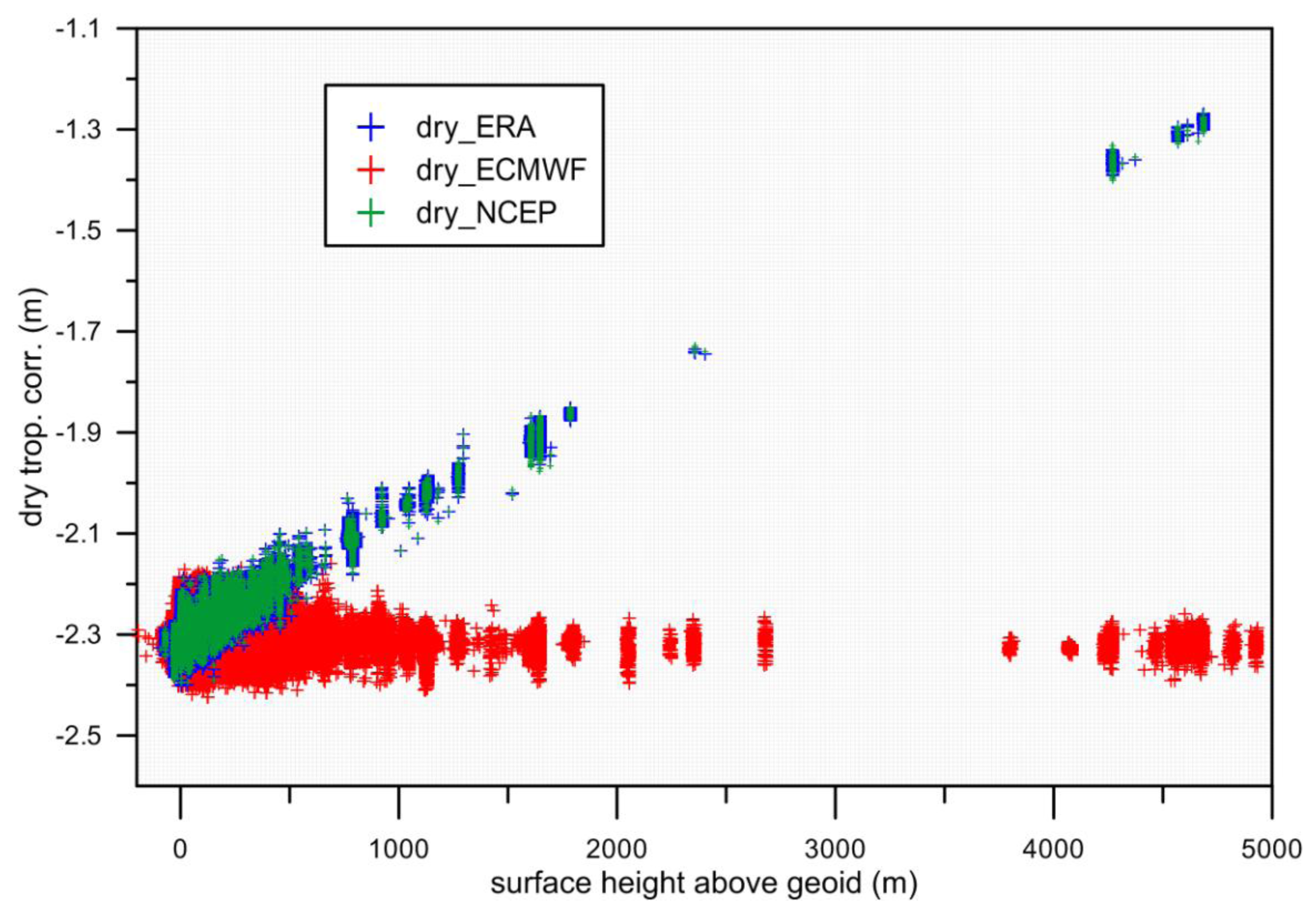
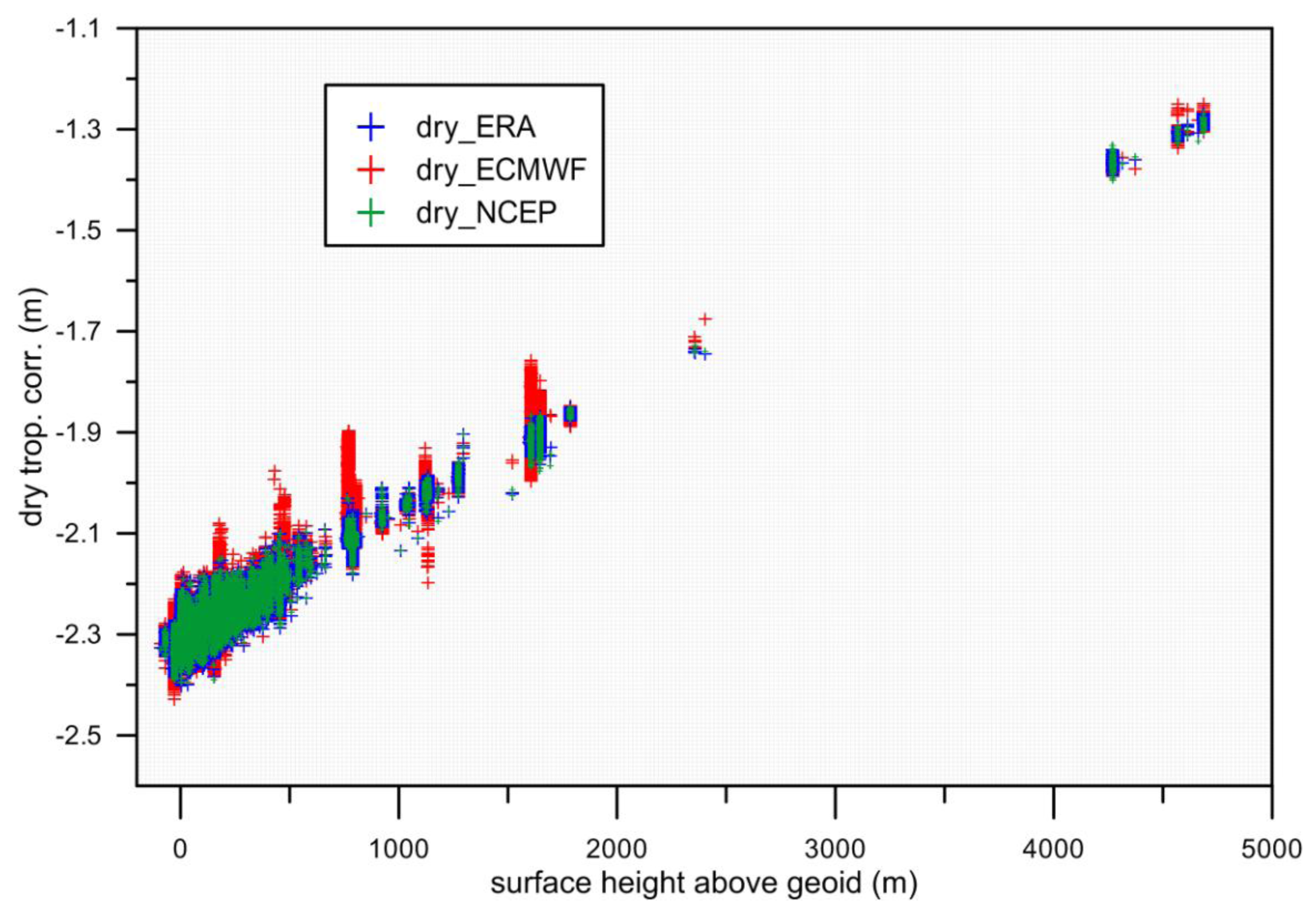
The DTC has been computed from SLP grids, with an expression similar to Equation (3) with no further reduction to the water surface level. For each location, this error is mainly a bias, which, for inland water at high altitudes, such as the Lake Titicaca (~3800 m), can reach 80 cm. Apart from a constant part, this error also has a seasonal component, since, according to Equation (6), an accurate height dependence of surface pressure can only be modeled by accounting for the seasonal variations of atmospheric pressure with temperature [43].

(2)

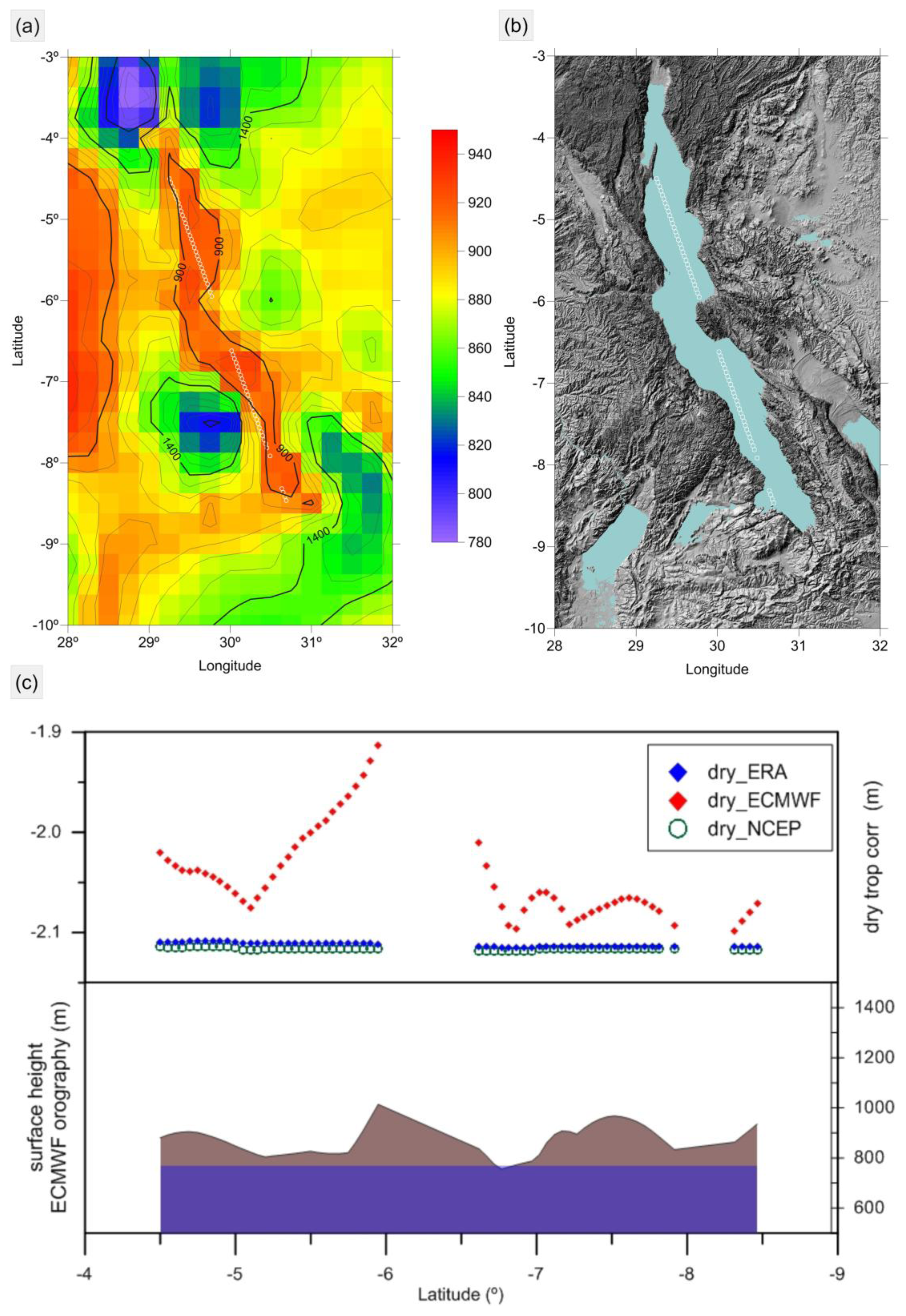
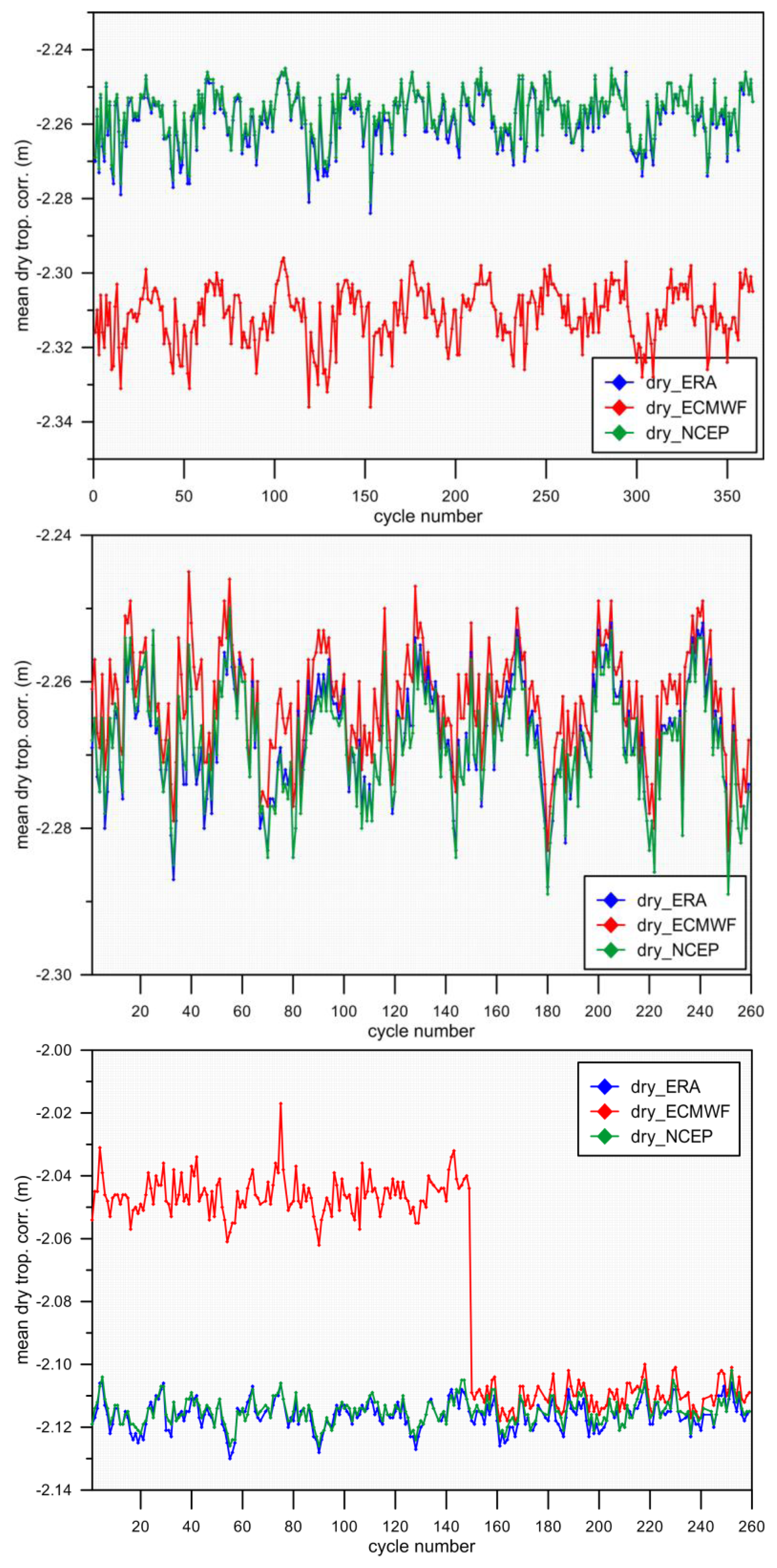
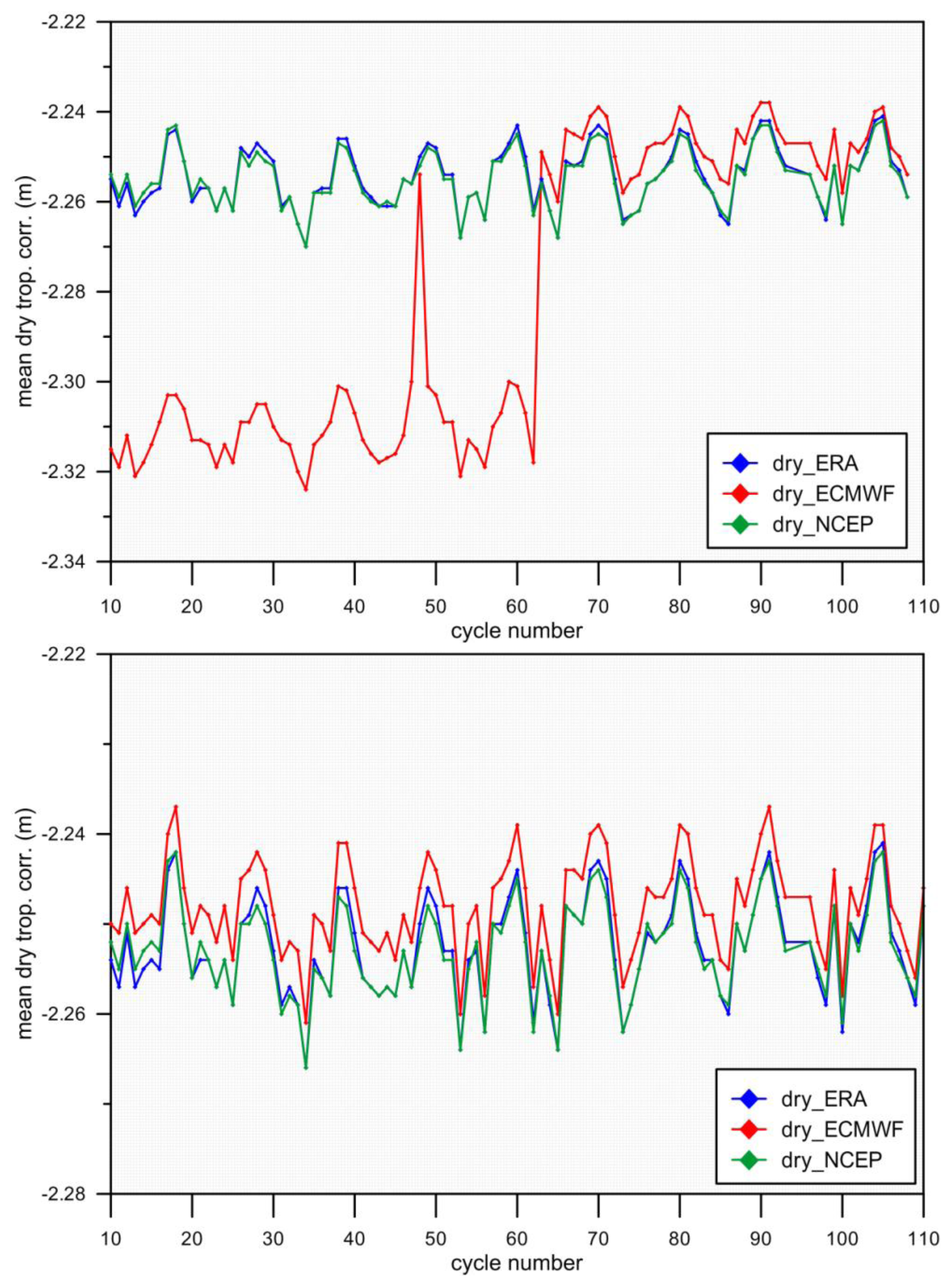
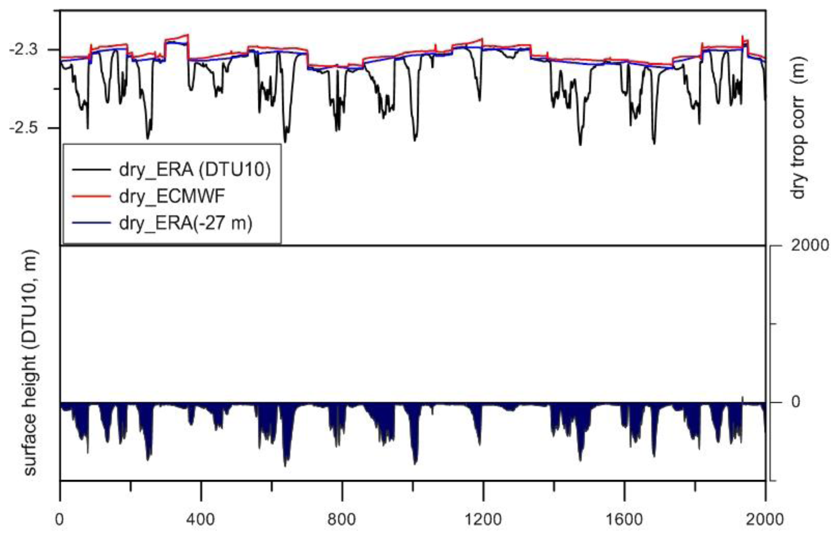
The DTC is estimated from surface pressure grids at the level of the model orography. This will induce interpolation errors, due to the fact that the model orography might depart significantly from the actual surface height. In regions of large variations in terrain height, such as a river in a deep valley or a lake surrounded by high mountains, even if the model orography correctly fits the terrain heights, there may be a large difference between the DTC at the points over the mountains and the DTC at the center of lake or river. This may cause along-track interpolation errors at the decimeter level, with a linear decrease/increase in the DTC as the points approach the center of the lake, reported as “V shape” errors by, e.g., [5], and illustrated in Figures 3 and 4 for Lake Tanganyika.

(3)

The DTC has been computed from SLP grids, with an expression, such as Equation (3), with further reduction to the surface water level, for each along-track altimeter location, using an appropriate height reduction. Studies by [43] show that, for heights up to 1000 m, Equation (6) provides the DTC with an accuracy of a few millimeters if an accurate DEM is adopted and the GPT climatological model is used to model the seasonal dependence of atmospheric pressure on temperature. Further research is required to find out how these results can be extended to larger heights, up to 4000 or 5000 m, since a few continental water regions of interest exist at these altitudes. Preliminary results indicate that for these altitudes, errors due to the inaccurate modeling of both the height and the temperature dependence of surface pressure are expected.

Figure 7 further illustrates the importance of using correct height information in the required height reduction of the DTC. This figure illustrates the DTC (top, in m) and surface topography from DTU10 (bottom, in m) versus the point number by ascending time order, over the Caspian Sea, for SARAL Cycles 1 and 2. The ECMWF Operational DTC values are those present in RADS, extracted from the (I)GDRs. The blue line represents ERA DTC computed using a mean height of −27 m, while the black line shows the ERA DTC values obtained using the DTU10 topography model in the computation of the height reduction. The difference between the red and blue lines (a mean value of 7 mm) reveals that the ECMWF operational DTC, present in the (I)GDRs, was computed using a mean height of 0 m.

In summary, to avoid most of the reported errors over inland water regions, the DTC for satellite altimetry should be computed as follows:

(1)

For each atmospheric model SLP grid node, compute the correction at sea level using Equation (3) and setting h_s = 0.

(2)

Interpolate for each altimeter measurement location.

(3)

Apply height reduction using Equation (6) and a model topography, such as DTU10 (apart from the Caspian Sea, where a mean sea height must be adopted). Users may also use a local and more precise DEM where available. For studies over lakes or reservoirs, for example, it will be preferable to use the mean lake height instead. In the implementation of Equation (6), the surface temperature can be obtained from the values of the temperature at mean sea level given by the GPT climatologic model and considering a mean normal lapse rate of temperature with height of −0.0065 K/m.

For non-time-critical inland water studies, the authors recommend the use of the correction from the ERA Interim model, which is more stable in time, although both the ECMWF operational and NCEP models provide enough accuracy, if the appropriate computation procedure is adopted. Alternatively, whenever measurements of surface pressure are available, from reliable and well-monitored barometric stations, these can be used to compute the DTC from Equation (3) with an accuracy of about 1 cm [7,43].

2.2. Wet Tropospheric Correction

2.2.1. WTC Estimation

The path delay due to the presence of water vapor in the atmosphere, the wet tropospheric correction (WTC), is one of the major error sources in satellite altimetry. With an absolute value less than 50 cm, it is highly variable, both in space and time. Due to this high variability, over the ocean, the most accurate way to model this effect is through the measurements of microwave radiometers (MWR) on board the altimetric missions.

The passive MWR on board altimeter missions retrieve the water vapor content from the instantaneous measured brightness temperatures, at the nadir, in channels inside and outside the water vapor absorption line centered at 22.235 GHz. An analysis of the errors associated with the WTC estimation from on-board MWR of various missions can be found, e.g., in [49].

Three-band radiometers have been used in the NASA/CNES/NOAA/EUMETSAT missions (T/P, Jason-1 and Jason-2): one at the water vapor line at 18–18.7 GHz (low sensitivity to clouds), one in the absorption line (21–23.8 GHz) and one in the 34–37 GHz band (as sensitive to the surface as the low frequency one, but more sensitive to cloud liquid water).

In the ESA missions (ERS-1, ERS-2 and Envisat) two-band radiometers have been used: 23.8 GHz and 36.5 GHz. GFO also carried a dual frequency MWR at 22 GHz and 37 GHz [50]. SARAL also carries a two-band radiometer (23.8 and 36.8 GHz) similar to that of Envisat, sharing the AltiKa antenna and allowing a smaller footprint [51].

CryoSat-2 does not carry a radiometer, thus relying on models, such as those from ECMWF. New approaches are being developed to determine the WTC for CryoSat-2, based on the combination of all available data types: from imaging radiometers on board remote sensing satellites, from models and GNSS-derived wet delays from inland stations [43,52].

The algorithms used to retrieve the WTC from the measured brightness temperatures of the various MWR channels assume a constant surface ocean or calm waters emissivity. Therefore, in the presence of surfaces with different emissivity, the measurements become invalid. This is the case of land, vegetation or ice surfaces.

The problems associated with the computation of the wet tropospheric correction in the coastal regions, where the MWR measurements also become invalid, in the context of missions possessing an on-board MWR, has been addressed by several authors [53–56]. These authors have derived algorithms for improving the WTC in the coastal regions, but these algorithms have not been customized for inland water regions.

Over continental waters, the wet path delay retrieval from passive microwave radiometers is hampered by the contamination on the radiometer measurements of the surrounding lands (e.g., in lakes or rivers), mixed vegetation in wetlands or ice at high latitudes. Because of its large footprint, the MWR measurements over an oceanic or lake surface become invalid, due to emerged lands, within distances of about 20–40 km of the water area limit, depending on the frequency. Consequently, the MWR correction provided in the GDRs is usable only in the central parts of very large lakes. In the case of smaller lakes (<2000 km²), the footprint of the radiometer always encompasses surrounding lands or islands, and then, the MWR-derived WTC is either not available or invalid. Thus, MWR-derived WTC cannot be used in small lakes or over river channels. In these regions, alternative sources must be used.

For regions possessing permanent GNSS stations, GNSS-derived wet path delays can be derived with an accuracy close to 1 cm, the same accuracy as MWR-derived WTC (e.g., [55]). This approach is particularly favorable for small lakes and reservoirs, where the measurements at a single location can be representative of the whole lake, the approach followed by, e.g., [7]. However, unlike the coastal regions, where GNSS data have been used in combination with other available wet path delay sources (valid MWR measurements in the vicinity of the point and model values) [55], so far, this procedure has not been exploited over inland water regions.

In the absence of any other data source, the WTC from meteorological models must be used. Although the overall accuracy of WTC from meteorological models is worse than the corresponding values from MWR, the quality of the recent models has been increasing significantly [34], particularly for the latest reanalysis product from ECMWF, the ERA Interim model [36,57].

For use in satellite altimetry, the WTC can be calculated from global grids of two single-level parameters provided by global atmospheric models, the total column water vapor (TCWV, expressed in mm or, the equivalent, kg/m²) and near-surface air temperature (two-meter temperature, T₀), from the following expression [58,59]:

$$\mathrm{\Delta }{R}_{wet}(h_S)=-\left(0.101995+\frac{1,725.55}{T_m}\right)\frac{\text{TCWV}}{1,000}$$

(8)

where T_m is the mean temperature of the troposphere, which can be modeled from T₀, according to, e.g., [60,61]:

$$T_m=50.440+0.789\hspace{0.17em}{T}_0$$

(9)

Equations (8) and (9) provide the WTC at the level of the atmospheric model orography. This orography may depart from the actual surface height by hundreds of meters. If accurate surface heights are available, the corresponding value at the surface can be obtained by an appropriate height reduction.

Unlike DTC, which has a relatively well-known height dependence (see Section 2.1), the height dependence of water vapor is not easy to model, due to its large variability. In spite of this, Kouba [39] proposed the following empirical expression:

$$\mathrm{\Delta }{R}_{wet}(h_s)=\mathrm{\Delta }{R}_{wet}(h_o)e^{\frac{h_o-h_s}{2000}}$$

(10)

where h_s and h₀ are the ellipsoidal heights of the model orography and surface, respectively. Thus, height errors of, e.g., 100 and 500 m, will induce errors of 5% and 28%, respectively (1 cm and 5.6 cm for a correction of 20 cm). Although these errors are considerable, in the altimetric products, the model-derived WTCs are commonly referred to the model orography or given at sea level, since in some regions it is difficult to have reliable DEM. According to [39], Equation (10) should only be used to performed WTC height reductions up to 1000 m.

In summary, for each model grid node, the correction is: (1) computed at the orography height using Equation (8), followed, or not, by a height reduction to the surface height by Equation (10); (2) interpolated at the altimetric measurement location; and (3) interpolated at the measurement time using the two closest model grids, six hours apart.

Alternative approaches for the computation of the wet path delay from other parameters provided by the global atmospheric models can be adopted, e.g., from 3D parameters (specific humidity, near-surface air temperature and surface pressure; see, e.g., Equation (1) in [62]). In this case, the integration over height can be performed from the top of the troposphere until the surface. In [62], a computation algorithm is proposed, where the effective thickness of the atmosphere column is deduced from the altimetric measurement itself.

2.2.2. Analysis of WTC Errors Present on Altimetric Products

Similarly to the analysis performed in Section 2.1.2 for the DTC, in this section, we present an evaluation of the WTC available on altimeter products, using the values provide in RADS as examples.

As summarized in Table 1, for each mission, RADS provides the wet tropospheric correction from the on-board MWR (if available) and from three models: ECMWF operational, ERA Interim and NCEP (apart from Geosat and GFO, where the values from the ECMWF operational model are not available, as they are not present in the corresponding GDR). In addition, as mentioned before, the MWR correction is not available for CryoSat-2.

As for the DTC, the WTC from ERA Interim and NCEP present in RADS have been calculated from the model grids, at 80 km and 2.5° spatial sampling and six-hour intervals. The values have been computed at the model orography height using Equations (8) and (9). For the ECMWF operational model, the values from each mission GDR are given without any change, except for CryoSat-2, for which the correction has also been computed directly from the model grids.

In the following analysis, a selection of points over inland water was made based on the same criteria as described in Section 2.1.2. In addition, in the analyses involving the measurements from the on-board MWR of each mission, only points for which the radiometer flag indicates no corruption by land were considered.

Figure 8 shows the mean WTC from each of the three analyzed models, for each 10-day cycle of T/P (Phase A), Jason-1 (Phase A) and Jason-2. The dominant feature is the strong seasonal signal of this correction, with a 12–15-cm peak-to-peak amplitude. Figure 9 shows the mean (top) and standard deviation (bottom) of the differences between the WTC from ERA and each of the other two models, for each 10-day cycle of T/P (Phase A), Jason-1 (Phase A) and Jason-2. Both figures show that the WTC from ECMWF is not provided in a consistent way in the GDRs of T/P, J1 and J2, the so-called reference missions. While for T/P, it is provided at sea level, for Jason-1 and Jason-2, they are correctly determined by integrating water vapor from the surface upwards (Table 1).

These results also show that, when computed at the same level as is done for Jason-1 and Jason-2, the differences between the ERA and ECMWF operational model decrease with time, with a mean of 0.4 cm and a standard deviation of 1.5 cm for the whole Jason-1 and Jason-2 period. These values are in agreement with the results obtained for the global comparison of the two models (not shown here), which shows that the ECMWF operational model has been updated and improved several times over the years. The global difference between the two models has a standard deviation, for each six-hour grid, that goes from 2.5 cm in 1995 to about 1.1 cm after 2004. The corresponding values shown in Figure 9 are somewhat larger than the global results and might be due to the different sampling and to the fact that the WTC from the two models might have been computed using different formulae.

Results also show that the differences between ERA and NCEP are larger than the corresponding differences between the ERA and ECMWF operational model (considering only these last ones for the Jason-1 and Jason-2 period). The differences between ERA and NCEP are stable in time, with a mean value of −0.6 cm and a standard deviation of 2.3 cm for the whole set of Jason-1 and Jason-2 cycles.

Figures 10–13 and

Table 2. Statistical parameters (in cm) of the comparison of the various WTC for Lake Victoria. Values refer to the differences for the following periods of each mission: T/P (Phase A), Jason-1 (J1; Phase A) and J2 (Cycles 1–183) and Envisat (EN; Cycles 10–93).

Models		Mean	Stand. dev.	Min	Max
T/P	MWR-ERA	−1.4	2.2	−11.1	5.1
	MWR-ECMWF	9.3	3.2	−1.8	20.8
	MWR-NCEP	−4.6	2.7	−14.5	4.7
J1	MWR-ERA	0.6	2.3	−19.2	8.7
	MWR-ECMWF	−0.5	2.1	−22.2	5.6
	MWR-NCEP	−3.2	2.8	−21.7	5.7
J2	MWR-ERA	0.3	2.0	−9.6	6.5
	MWR-ECMWF	−0.6	1.6	−9.0	6.2
	MWR-NCEP	−2.8	3.0	−13.8	6.1
EN	MWR-ERA	1.3	4.1	−19.8	11.5
	MWR-ECMWF	0.1	4.0	−25.9	9.8
	MWR-NCEP	−1.8	4.4	−27.6	9.7

and

Table 3. Statistical parameters (in cm) of the comparison of the various WTC for the Caspian Sea. Values refer to the differences for the following periods of each mission: T/P (Phase A), J1 (Phase A) and J2 (Cycles 1–183) and Envisat (EN, Cycles 10–93).

Models		Mean	Stand. dev.	Min	Max
T/P	MWR- RA	0.4	1.6	−18.1	8.8
	MWR-ECMWF	0.3	2.0	−18.6	10.0
	MWR-NCEP	−0.8	2.9	−18.5	9.0
J1	MWR-ERA	0.3	1.8	−17.8	8.5
	MWR-ECMWF	0.6	1.7	−18.5	11.4
	MWR-NCEP	−0.5	3.4	−22.8	11.0
J2	MWR-ERA	0.3	1.8	−17.8	9.1
	MWR-ECMWF	0.5	1.4	−9.2	10.7
	MWR-NCEP	−0.4	3.2	−21.2	9.3
EN	MWR-ERA	0.5	3.2	−20.0	9.5
	MWR-ECMWF	0.8	3.1	−22.9	11.1
	MWR-NCEP	−0.1	4.0	−28.0	9.3

show the comparison between the WTC from three models and from the on-board MWR of each mission for Lake Victoria (Africa) and the Caspian Sea. These are examples of two regions with significantly different conditions for various range corrections, including the WTC.

Lake Victoria is one of the world’s largest lakes, located in Africa, with a mean height of about 1135 m. Over this lake, the WTC has a weak seasonal signal, with values between 10 cm and 30 cm all over the year (Figure 10). Over this lake, all models capture very well the main wet path delay variations revealed by the MWR correction, except for some wetter conditions.

Results show that the T/P correction from the ECMWF operational model is too negative by about 10 cm (Figures 10 and 11 and Table 2), since it is provided at sea level instead of lake height. The authors of [5] reported a similar behavior of the ECMWF WTC on the T/P GDR, which also provided the correction at sea level, derived from global 3D grids.

From the three models, ERA is the one providing the best results, with a mean difference with respect to MWR, considering the whole analyzed period from 1992 to 2013, of 0.0 cm and a standard deviation of 2.3 cm. The corresponding statistics for the difference between MWR and NCEP are −3.4 cm for the mean and 2.9 cm for the standard deviation. Thus, although in terms of variability, ERA and NCEP seem to be similar over Lake Victoria, NCEP has a bias of about 3 cm with respect to ERA and MWR.

The Caspian Sea has a mean height of −27 m. The most striking feature of the WTC over this closed sea is its strong seasonal signal with a peak-to-peak amplitude close to 15 cm (Figures 12 and 13). Regarding the ECMWF operational model, due to the small sea level height, the fact that the correction is provided at sea level does not introduce any significant error.

As for Lake Victoria, from the three models, ERA is the one that provides the best results (Figure 13 and Table 3), with a mean difference with respect to MWR of 0.3 cm and a standard deviation of 1.7 cm, considering the period from 1992 to 2013. The corresponding statistical parameters for the difference between MWR and NCEP are −0.5 cm for the mean and 3.2 cm for the standard deviation. Figure 13 shows that the amplitude of the differences of NCEP with respect to MWR is considerably larger than those for the other two models, showing that NCEP is not able to model the large seasonal variations present in the WTC of the Caspian Sea. The results obtained for the ECMWF operational model are of the same order of magnitude of those obtained for ERA, showing that when provided at the same level and for the period after 2004, these two models provide similar results.

Concerning other altimetric missions, no systematic differences were found between the WTC from the three analyzed models for Envisat, CryoSat-2 and SARAL, thus indicating that these corrections are provided at surface height and should have an accuracy close to that of Jason-1 and Jason-2. As shown in Tables 2 and 3, for Envisat and, generally, for all 35-day missions, the standard deviations of the differences between the MWR correction and each model are larger than the corresponding values for the reference missions by a factor of 1.5–2.0. This can be explained by the fact that these missions have many more passes over these regions, thus spanning a larger range of conditions and mostly because the MWR correction of these missions is much more affected by land effects than the corresponding corrections for the reference missions. Thus, these larger standard deviations cannot be just attributed to model errors, but also to MWR land contaminated measurements that have not been properly edited by just using the radiometer land flag. In spite of the consistency between the three models for all these missions, for Envisat, before 2004, the accuracy of the correction from the ECMWF operational model gets worse, while ERA Interim and NCEP have the same accuracy for the whole missions lifetimes.

For all inland water measurements of the ERS-2 and ERS-1 analyzed cycles over Lake Victoria, a bias around 10 cm was found between the ECMWF operational model and ERA Interim, as reported for T/P, suggesting that for these satellites, the WTC from ECMWF operational model is provided at sea level.

In summary, considering the best available atmospheric model, ERA Interim, results based on the differences between the WTC from the on-board MWR and the model-based wet path delay indicate that the WTC can be estimated over continental waters with an overall accuracy (one standard deviation) of 1 to 3 cm, depending on the region. Moreover, like all models, ERA may have local biases of 1–3 cm. For studies using data only after 2004, the best option is the ECMWF operational model, provided the correction is properly estimated at surface height, due to its higher spatial resolution compared to ERA Interim. The limitation of ERA Interim is its spatial resolution (~80 km), which may not resolve short wavelength variations in the WTC, particularly critical in regions of strong water vapor variability, such as the tropics.

The ECMWF operational model provided in the GDR products of the various missions is not provided consistently and must be used with caution, particularly on T/P and ERS products. Here, the ECMWF-derived WTC is provided at sea level, and the correction by the user to surface height using Equation (7) and a suitable DEM does not provide enough accuracy for heights above 1000 m [39].

For inland water studies, the authors recommend the use of the MWR-derived wet tropospheric corrections, using appropriate editing, where available (over large lakes and closed seas), or GNSS-derived wet path delays whenever GNSS stations exist in these regions.

In all other cases, in particular over rivers, small lakes and wetlands, the ERA Interim model, computed at the model orography, as described in this section, can be used. Alternatively, as suggested by [62], the correction can be estimated at surface height using 3D parameters. In this case, the integration can be performed over height, from the surface to the sensor, and more realistic surface heights can be used, for example those derived from the altimeter measurements. This procedure has the advantage that the height dependence of the WTC is modeled with higher accuracy, but requires a larger computational effort, and altimeter-derived surface heights must be used with caution, with an appropriate editing criterion.

2.3. Examples of Case Studies

Aiming to illustrate the effective impact of the tropospheric correction errors on altimeter water level measurements, in this section, two case studies are presented: for Lake Victoria and for Lake Tanganyika. Since the major tropospheric errors were found in the T/P products, data from T/P, J1 and J2 have been used in these examples.

For the so-called reference orbit, each mission has mainly only one pass, Pass 120 over Lake Victoria and Pass 222 over Lake Tanganyika. Since only 1-Hz measurements were used from the RADS database, the relatively small number of available measurements limits the results. For this reason, in the water level time series, instead of the mean, the median values are represented.

For each of the mentioned lakes, altimeter data have been extracted from RADS using the criteria described in Section 2.1.1. For each measurement point, three sets of water level heights above the EGM2008 geoid were computed, using the default RADS orbit and a common set of corrections: ionosphere (JPL_GIM), solid Earth tide, load tide (GOT4.8) and pole tide. Then, for each data set, the dry and wet tropospheric corrections were computed from each of the three analyzed atmospheric models: ECMWF operational, ERA Interim and NCEP.

Figures 14 and 15 illustrate the impact of the corrections on the determination of water level time series. As discussed in the previous sections, the fact that in the T/P GDRs, the tropospheric corrections from ECMWF are provided at sea level causes a bias (39 cm for Lake Victoria and 26 cm for Lake Tanganyika). The actual errors are not exactly constant, since, e.g., the height dependence of the wet tropospheric correction is a function of the correction itself, Equation (10); therefore, for wetter conditions, the errors are larger than for dryer conditions. However, when computing the mean for, e.g., a 10-day cycle, the errors nearly average out. When deriving time series from various missions, for which the corrections are not consistent, the impact on the water level time series is evident, with a significant impact on the long-term water level trend. This effect is larger for Lake Victoria, since it is at a higher elevation than Lake Tanganyika.

Figures 16 to 18 illustrate the impact of different types of tropospheric errors in the determination of mean lake profiles. Three examples are given for Pass 222 over Lake Tanganyika.

Figure 16 shows the impact of providing the corrections at sea level instead of at lake height, as happens for the ECMWF corrections from T/P GDR. Apart from a large bias of ~26 cm, the difference between the water level height computed, e.g., from ECMWF and ERA Interim, has a pattern related to the ERA Interim orography used in the WTC computations from this model. Results for NCEP are not shown, since they are very similar to those from ERA Interim.

Figure 17 illustrates the errors associated with the computations of the DTC from surface pressure grids. In this case, the pattern of the differences is due to the difference between the ECMWF model orography and the actual mean lake height. The amplitude of these errors can reach the decimeter level (see also Figure 4). Figure 18 shows the impact of the changes introduced in the J1 processing after the end of Cycle 149, largely correcting the previously mentioned errors (see also Figure 3, bottom plot).

In summary, Figures 16 to 18 show that the errors introduced by the inadequate computation of the tropospheric corrections are not just a bias and may have large along-track variations. These types of errors may have a strong impact on comparisons of altimeter data with in situ data, such as, e.g., in altimeter calibration sites over lakes.

3. Ionospheric Correction

3.1. Estimation of the Ionospheric Correction

As part of the range estimation for satellite altimetry, which enables the inland water level (or stage) to be estimated, the refraction caused by the presence of electrically-charged particles in the atmosphere has to be accounted for. Most of those charged particles occur in the so-called ionosphere, the part of the atmosphere between an altitude of ~50 and 2000 km, where ions are produced by the photoionization of atomic and molecular gasses [63].

The total delay affecting the altimetric radar pulse along its path through the ionosphere, ΔR_ion, can be estimated from the integral over height, from the target to the sensor, of the ionospheric refractivity N_ion(z), which is, in turn, proportional to the density of electrons in the ionosphere, n_e(z). Unlike its hydrostatic and wet counterparts, the ionospheric refraction is frequency-dependent, i.e., the ionosphere is a dispersive medium for the propagation of the radar pulse, the ionospheric refractivity being inversely proportional to the square of the frequency, f, of the propagating signal (e.g., [13]):

$$\mathrm{\Delta }{R}_{\text{ion}}(f)={10}^{-6}{\int }_0^R{N}_{\text{ion}}(z)\hspace{0.17em}\text{d}z=\frac{k}{f^2}{\int }_0^R{n}_{\text{e}}(z)\hspace{0.17em}\text{d}z$$

(11)

where k = 40.250 m³ · Hz² · electrons⁻¹, n_e is expressed in electrons/m³, f in Hz and ΔR_ion results in meters. The last integral in Equation (11) represents the atmospheric columnar electron density, i.e., the number of electrons per unit area in a column extending from the surface of the Earth to the altimeter. This total electron content (TEC) is usually expressed in TECU (TEC units), with 1 TECU = 10¹⁶ electrons/m², allowing the altimetric ionospheric path delay to be more practically written as in Equation (12):

$$\mathrm{\Delta }{R}_{\text{ion}}(f)=\frac{k\hspace{0.17em}{\text{TEC}}_{\text{alt}}}{f^2}$$

(12)

where k = 0.40250 m·GHz²·TECU⁻¹, f is expressed in GHz, and TEC_alt is the total electron content below the altimeter (in TECU), yielding ΔR_ion in meters. For altimeters operating in the Ku-band (approximately 13.6 GHz), this comes out to 2.18 mm of path delay per TECU (e.g., [64]). Operating on two different frequencies, recent high-precision radar altimeters flying on Envisat, Jason-1, Jason-2 and TOPEX allow, in principle, direct estimation of TEC_alt from the difference between the measured ranges on the two frequencies [28]:

$${\text{TEC}}_{\text{alt}}=\frac{f_{\text{Ku}}^2\hspace{0.17em}{f}_{\text{C},\text{S}}^2}{f_{\text{Ku}}^2-f_{\text{C},\text{S}}^2}\frac{R_{\text{C},\text{S}}-R_{\text{Ku}}}{k}$$

(13)

The ranges, R_Ku and R_C,S, in Equation (13) are those measured on the primary Ku-band and on the secondary C-band (5.3 GHz for TOPEX and Jason) or S-band (3.2 GHz for Envisat), respectively, neglecting the effects of atmospheric refraction. The above formulation has been the primary source of estimation for the ionospheric path delay for ocean altimetry performed by dual-frequency altimeters, as the necessary correction can be retrieved simultaneously, i.e., coincident in space and time, with the range measurements. Unfortunately, the range measurements at the secondary frequencies are inherently less precise than those at the Ku-band frequency, such that the dual-frequency path delay correction would create a much noisier sea level determination. Therefore, in order to reduce the cumulative error arising from the instrumental noise at the two radar frequencies, the dual-frequency retrieved ionospheric correction is usually smoothed with the use of an along-track low-pass filter over about 140–200 km (approximately 20–35 s), as first suggested by [65].

Single-frequency altimeters (such as CryoSat-2, ERS-1, ERS-2, Geosat, GFO and Poseidon) must rely on independent estimates of TEC_alt for the ionospheric range correction, as those available from observational or climatological global models. AltiKa, on board SARAL, is a special case, as unlike all other single-frequency satellite altimeters, it is operating in the Ka-band (35.75 GHz) and is thus about seven times less affected by the ionosphere than Ku-band altimeters, approximately 0.31 mm of path delay per TECU, as determined by Equation (12).

The first attempts to model the ionosphere were based on the development of climatologies, e.g., the Bent model [29,30] and the International Reference Ionosphere (IRI) (e.g., [66–68]). Neither of these climatologies ever included GNSS data. However, just like the dual-frequency altimeters, the dual-frequency GNSS measurements provide an abundance of TEC observations along the slant-ranges, and since 1998, institutions like the Jet Propulsion Laboratory (JPL) and the University of Berne started the operational production of global ionosphere maps (GIM) of vertical TEC based on those GNSS slant-range observations. At present, JPL GIM are produced from a global network of about 170 stations and 31 GNSS satellites that contribute their data through the International GNSS Service (IGS) and other institutes [69,70]. Since 28 August 1998, two-hourly GIM maps are available from JPL with a single-layer gridded solution of 2.5° spacing in (geocentric) latitude and 5° in longitude [70,71]. More recently, NIC09 (NOAA Ionosphere Climatology 2009), a global climatological model based on JPL GIM for the period 1998–2008, has been developed by [28], which can provide global TEC maps with the same spatial and temporal resolutions as JPL GIM, allowing, in addition, the estimation of ionospheric path delays prior to 1998. While GIM uses actual measurements of the total electron content (TEC) along slant-paths through the atmosphere and then models the vertical TEC from that, the NIC09 uses a proxy of the solar activity (global mean electron content or a combination of solar flux and geomagnetic index), a single value for a given time, and then models the global distribution of the vertical TEC based on season and time of day.

In order to use GNSS-derived TEC to estimate the ionospheric correction for altimeter range measurements, besides the necessary interpolation in space and time to the altimeter ground track, additional altitude scaling has to be performed [27], since GNSS measurements integrate TEC to an altitude of about 20,200 km, whereas the altimetric satellites fly only at 1350 km (T/P, Jason-1 and Jason-2) or 800 km (most others). The approach by [27], based on the climatological model, IRI95 [72], suggests that there are essentially no free electrons above 1400 km, and thus, no altitude scaling is needed for the high flying altimeters (T/P and Jason). As for the low flying altimeters, the scaling factor to be applied in the retrieval of TEC_alt from the GNSS-derived TEC is the ratio of TEC_{IRI95 < 800 km} to TEC_{IRI95 < 1400 km}. However, [28] demonstrated, by comparing dual-frequency altimeter estimates (from TOPEX, Jason-1 and Envisat) and GIM TEC data, that about 8% of the TEC extends above 1350 km and about 14% above 800 km, thus suggesting the adoption of scaling factors of 0.925 for altimeters around 1350 km, and 0.856 for those around an altitude of 800 km. For CryoSat-2, flying around an altitude of 730 km, this factor is 0.844.

The vertical TEC that determines the ionospheric correction to be applied to the altimeter range measurement is known to exhibit large spatial and temporal variations. As illustrated on the global maps of Figure 19, the ionospheric delay presents a latitudinal dependence, varying by a factor of four and with maxima occurring along two bands paralleling the geomagnetic equator. Towards the poles, both the mean and the variation become smaller.

Despite the relative homogeneity of its temporal mean, local ionospheric delays are prone to exhibit large variations, depending on season of the year, time of day and solar activity. The annual variation is mainly due to the changing orientation of the sun with respect to the geomagnetic field, being in general relatively small. However, seasonal variations are very significant in polar regions, where summer levels of TEC can be five times higher than the winter levels. Diurnal TEC variation is quite pronounced, generally peaking around 14:00 local time, with the highest level up to ten times the lowest, occurring around 02:00 during the night. The dependency on solar activity is mostly related to the 11-year cycle in solar radio flux, with levels for high activity periods going up to about five times those of low activity (see Figure 20). For the whole ionosphere, TEC values can range from one TECU during the night time to about 180 TECU in daytime during peak periods of solar activity [28].

In a comparison recently performed by [28], the RMS error of TEC models was shown to be more or less proportional to the TEC itself, with the RMS error of 14% to GIM, 18% to NIC09 and 35% to IRI2007. Therefore, from 1998 onwards, whenever dual-frequency measurements are not available or cannot be used to derive reliable ionospheric range corrections, properly interpolated and scaled GIM TEC data provide the more accurate alternative. Prior to that, one has to rely on less accurate climatological models, with increased error for periods of high solar activity, as ionosphere climatologies, tuned to model the lower TEC conditions, were shown to have a tendency to underestimate higher TEC values, IRI2007 significantly more so than NIC09 [28].

3.2. Analysis of Issues Regarding the Computation of the Ionospheric Correction over Inland Waters

As the ionosphere is insensitive to coastlines or surface topography, its effect on the propagation of the altimetric radar pulse, unlike those of the troposphere (wet and hydrostatic) does not depend on the altitude of the target, nor is it sensitive to any near-surface atmospheric currents. However, originally designed for ocean applications, the Ku and C (or S) radar altimeter bands have their range measurements differently affected by land. As a consequence, for inland waters applications, the accuracy of the estimation of the ionospheric path delay from the dual-frequency range difference, as detailed in Equation (13), is constrained both by the contamination of the returned radar pulse by land within the altimeter footprint and by the ability to perform the necessary along-track smoothing of the difference of the two range measurements (e.g., [73]).

Pioneering inland water altimetry applications (e.g., [1,74]) have relied mostly on climatologies or data derived from DORIS to compensate for the effect of the ionosphere, while others (e.g., [21]) relied on the smoothed dual-frequency altimeter data. With the extension of the time series of altimetric data and the consequent availability of GNSS-derived TEC, the more accurate GIM data became the preferred data source for the ionospheric correction of the range measurement (e.g., [3,75–77]), and the DORIS-derived ionospheric correction is no longer reported on the altimeter data products due to its relatively reduced accuracy. Although most of the authors using altimetry data for inland waters studies do not rely on altimeter dual-frequency-derived ionospheric correction, as part of a calibration study performed over Lake Issykkul, Cretaux et al. [5] compared the use of the altimeter dual-frequency ionospheric correction with that derived from GIM data, for Envisat and Jason-1. Their analysis is based on the comparison of the absolute bias of the altimeters (as deduced from GPS campaigns) when each of the ionospheric corrections available in the respective GDRs is applied. In that case study, GIM was shown to produce lower absolute Ku-band range measurement biases than dual-frequency (46.9 vs. 48.1 cm for Envisat and 5.4 vs. 7.0 cm for Jason-1) for the short, and low solar activity, period tested (September 2004, and September 2005). Studies by [16], as part of their validation exercise of Jason-2 altimeter range data over inland water bodies, show that for large unfrozen lakes, the dual-frequency instrument-based correction presents a much higher variability than that derived from GIM. As part of the same study, the particular case of Lake Ontario is also referred to as a case in which the use of the GIM-derived ionospheric improves the RMS of the estimated lake height (when compared to ground-based gauge data) by ~1.5 cm over the application of dual-frequency ionospheric correction. In their absolute calibration campaign of the Jason-1 and Jason-2 altimeters over Lake Issykkul, Cretaux et al. [6] further compared the use of the dual-frequency ionospheric corrections and those derived from GIM. Considering only altimeter data 10 km off the coastline and further filtering for outliers (differences larger than 5 cm), the authors found an agreement relative to GIM of about 1.1 cm for Jason-1 [7] and 0.4 ± 1.1 cm for Jason-2, over the period of August 2008 to August 2010. Moreover, due to the occurrence of errors of several centimeters in the retrieval of the dual-frequency ionospheric correction, affecting about 10% of Jason-2 data and even more for Jason-1, the GIM correction was selected as the most appropriate for their study.

In order to make a more definitive statement about the preferred ionospheric correction for inland water studies, we compared lake level measurements from Envisat and Jason-1, while applying various ionospheric corrections: JPL-GIM data scaled for the altitude of the satellite orbits as recommended by [28], dual-frequency altimeter data and the same dual-frequency data smoothed by averaging valid lake returns over the entire track crossing the lake. The best way to gauge the relative errors in each of the approaches consists in differencing lake levels at cross-over locations on the satellite ground tracks of the same altimeter, shortly enough spaced in time so that the lake level will not have substantially changed in the meantime. That time lapse was limited to half the length of the repeat cycle: five days in the case of Jason-1; 17.5 days in the case of Envisat. The measured lake level differences on these crossing points, known as crossover height differences, were used as a measure of the quality of the measurements: the lower the RMS crossover height difference, the more precise the measurements. Unfortunately, only the Great Lakes are a large enough body to have a substantive amount of crossovers to do this. An oceanic region with a similar size and latitudinal domain was also selected for comparison, and the results are presented in

Table 4. Standard deviations (in mm) of the crossover height differences for Jason-1 and Envisat during the years 2003–2004, using JPL GIM, non-smoothed dual-frequency range measurements and smoothed dual-frequency range measurements for the correction of the ionospheric refraction. The N-W Atlantic Ocean region (52°–40°W, 41°–49°N) is shown for comparison.

Jason-1	JPL GIM	Dual-Frequency	Smoothed Dual-Frequency
N-W Atlantic	88.5	89.2	85.5
Great Lakes	64.2	64.0	64.3
Envisat	JPL GIM	Dual-Frequency	Smoothed Dual-Frequency
N-W Atlantic	129.5	129.7	129.3
Great Lakes	62.9	63.1	62.7

for a two-year period of median solar activity (2003–2004). The water level in the Great Lakes varies roughly annually, with an amplitude of about 50 cm. Given the general distribution of the time difference of the crossovers, this contributes about 3 cm to the RMS figures presented for Envisat; less for Jason-1.

According to the presented results, the conclusions inferred for inland waters are not, in essence, different from what was already known (and again shown) for ocean applications. Whenever dual-frequency derived ionospheric correction can be retrieved and smoothed, its use yields a slightly better range estimation (lower RMS error) than what is obtained with GIM. However, over smaller lakes, and certainly over rivers, it will not be possible to smooth the dual-frequency correction sufficiently to bring the noise down. In addition, land-contamination of the C- (or S-) band signal is of concern, as well, similar to coastal regions [14]. Thus, the impact of smoothing the dual-frequency ionospheric correction over inland waters is less pronounced than over ocean. Only over very sizeable water bodies, like the Great Lakes in the example, smoothing can be expected to be effective enough to bring the crossover RMS error down below that obtained with the GIM-derived correction. Even over the Great Lakes, the differences in the standard deviation of the crossover height differences are small: 0.1 and 0.2 mm for Jason-1 and Envisat, respectively. These results largely confirm what was suggested earlier [5,16], that the ionospheric correction based on JPL GIM was to be preferred for inland waters. However, we like to stress that for large bodies of inland water (200 km and larger, like the Great Lakes), the smoothed dual-frequency ionospheric correction can still provide better results.

Another possibility that could be further investigated is the use of regional GNSS-derived models for the ionospheric correction of inland water altimetry. With the enhanced GNSS coverage in Europe and North America, regional ionosphere maps (RIMs) can be produced at a much finer spatial and temporal resolution in these areas. The RIMs produced since 2004 for Europe (30°–70°N; 15°W–40°E) by the SPECTRE project (Service Products for ionospheric Electron Content and Troposphere Refractivity over Europe) were shown to better resolve small-scale variations of the ionosphere than the JPL GIMs (e.g., [78]).

In conclusion, in agreement with previous studies, the authors recommend using the GIM-derived ionospheric correction over inland water bodies, for dual- and single-frequency altimeters alike. This avoids the possibility of land contamination in the C- or S-band footprint, as well as the limited number of points over which to smooth the dual-frequency correction. For the correction of altimeter measurements prior to the availability of GIM data (1998), the use of NIC09 is recommended. One should be aware that the GIM-derived ionospheric correction provided on most TOPEX, Jason-1 and Jason-2 GDR products is not reduced for the TEC extending above the altitude of these satellites, thus overestimating the ionospheric correction by about 8%.

4. Discussion and Conclusions

For inland water (IW) studies using satellite radar altimetry, in addition to the atmospheric corrections, the most relevant corrections are those from solid Earth, ocean tide loading and lake tide, if applicable. The dynamic atmospheric correction is not applied, because the lakes/reservoirs are closed systems. The SSB is usually also not applied, because wind effects tend to be averaged out along-track [15], although recent studies made by the authors, outside the scope of this paper, indicate that for regions, such as the Great Lakes, the application of the SSB correction slightly reduces the lake level height anomaly variance at the crossovers.

It has been shown that the tropospheric corrections are not modeled and computed properly and in a consistent way in the various altimetric products, as reported by many authors. If not appropriately corrected, they may be the main source of error for IW applications. In contrast to the ocean domain, IW studies require the modeling of the height dependence of tropospheric corrections. Since most radar altimeter products have been designed for oceanographic purposes, they often fail to provide valid corrections over continental water regions.

While over the ocean, the DTC is one of the most precise range corrections (better than 1 cm), in some of the present altimeter products, it is the correction with the largest errors for IW studies, up to several decimeters. It has been shown that the DTC determined from model grids may possess mainly two types of errors: (1) large biases if it is provided at the sea instead of at the surface level; and (2) interpolation errors with a strong along-track signature, when it is given at the level of the model orography and has been computed from surface pressure grids.

Users must be aware that the DTC derived from the ECMWF operational model is not provided homogeneously on the GDR of the various missions. When provided at sea level, it can be reduced to surface height by applying an appropriate height reduction. However, when provided at the model orography, it is difficult to correct for the interpolation errors that might occur. Therefore, for IW studies, the DTC should be derived by first computing the correction at each altimeter measurement location by interpolation from SLP model grids and then performing a suitable height reduction, preferably using Equation (6), which accounts for the seasonal variations of pressure with temperature. Due to model stability, the use of the DTC from ERA Interim, as provided in RADS, is recommended.

Due to its large spatiotemporal variability, the WTC may be the second largest source of error over IW regions. Being the best correction over the ocean, MWR-derived WTC should also be adopted whenever available, over the largest lakes, such as the Great Lakes and Lake Victoria. In regions possessing GNSS permanent stations, GNSS-derived WTC can be a very valuable and accurate data source, particularly, e.g., for small lakes for which the data from a single station is representative of the local wet path delay conditions. In the absence of any of the previous data types, over small lakes and rivers, model-derived corrections from the ERA Interim, computed at surface height, provide the highest accuracy (1–3 cm).

The WTC from ECMWF operational model provided in the GDR products of the various missions is not given consistently and must be used with caution, particularly on T/P and ERS products. Here, the ECMWF-derived WTC is computed at sea level, and the correction to surface height using Equation (11) does not give enough accuracy for heights above 1000 m [39]. When properly given at the model orography or at surface height, for the latest years (since 2004), the ECMWF operational model provides similar or better results compared with ERA Interim, while the NCEP model available in RADS is less accurate than any of the other two ECMWF products.

While over the ocean, smoothed dual-frequency instrument-derived ionospheric correction is the most accurate, the fact that the terrain has different effects on Ku- and C-/S-bands and the difficulty in performing an efficient smoothing over inland water regions make this correction unsuitable for use in most of these regions. Thus, from 1998 onwards, whenever dual-frequency measurements are not available or cannot be used to derive reliable IC, properly interpolated and scaled (as recommended by [28]) GIM TEC data provide the best source for the ionospheric path delay. Prior to that, the climatological model NIC09 can be used, with increased errors for periods of high solar activity.

This paper has addressed the main issues in the atmospheric corrections present in the products of the current altimetric missions, for studies over continental water surfaces, with emphasis on the missions most suitable for these studies.

In spite of the fact that CryoSat-2 does not carry an on-board MWR, the unique characteristics of its data makes them of great interest for inland water studies due to the fact that it operates in three modes [79]. For IW studies, the synthetic aperture radar (SAR) mode is of particular relevance, providing measurements with lower noise and improved spatial resolution of 300 m in the along-track direction, over pre-defined regions of interest, including IW regions such as the Amazon basin.

Concerning future missions, an altimeter similar to that of CryoSat-2 is planned for Sentinel-3, currently planned to be operating continuously in SAR mode, while Jason-CS (Jason Continuity of Service) is expected to operate for the first time in the so-called interleaved mode, where the satellite is capable of performing simultaneous and continuous measurements both in the traditional and SAR modes. These missions will increase the capability of acquiring measurements over IW surfaces with increasing accuracy and spatial resolution. A correct handling of all range and geophysical corrections, in particular those from the atmosphere, is crucial in the exploitation of these datasets.

Hydrological studies will reach a new era with the launch of the Surface Water and Ocean Topography (SWOT), a Ka-band wide-swath radar interferometer that will provide sea surface heights (SSH) and terrestrial water heights over a 120 km-wide swath with a gap of approximately 10 km around the nadir track. Over the deep oceans, it will provide SSH with a resolution of 2 m in along-track directions, while in the cross-track direction, the resolution will range from 10 m in the far swath to 60 m in the near swath. Over land, it will produce a water mask able to resolve 100-m rivers and 1-km² lakes, wetlands or reservoirs. Associated with this mask, water level elevations with an accuracy of 10 cm and a slope accuracy of 1 cm/km will be available. This high spatial resolution sets new requirements for the range and geophysical corrections. For this purpose, SWOT will carry a new type of radiometer with additional high frequency channels, to allow for a smaller footprint and improved water vapor retrieval in the coastal regions and over inland waters.

References and Notes

1. Birkett, C.M. The contribution of TOPEX/POSEIDON to the global monitoring of climatically sensitive lakes. J. Geophys. Res.: Oceans 1995, 100, 25179–25204. [Google Scholar]
2. Cazenave, A.; Bonnefond, P.; Dominh, K.; Schaeffer, P. Caspian sea level from TOPEX-POSEIDON altimetry: Level now falling. Geophys. Res. Lett 1997, 24, 881–884. [Google Scholar]
3. Calmant, S.; Seyler, F. Continental surface waters from satellite altimetry. C. R. Geosci 2006, 338, 1113–1122. [Google Scholar]
4. Cretaux, J.F.; Birkett, C. Lake studies from satellite radar altimetry. C. R. Geosci 2006, 338, 1098–1112. [Google Scholar]
5. Cretaux, J.F.; Calmant, S.; Romanovski, V.; Shabunin, A.; Lyard, F.; Berge-Nguyen, M.; Cazenave, A.; Hernandez, F.; Perosanz, F. An absolute calibration site for radar altimeters in the continental domain: Lake Issykkul in Central Asia. J. Geodesy 2009, 83, 723–735. [Google Scholar]
6. Cretaux, J.F.; Calmant, S.; Romanovski, V.; Perosanz, F.; Tashbaeva, S.; Bonnefond, P.; Moreira, D.; Shum, C.K.; Nino, F.; Berge-Nguyen, M.; et al. Absolute calibration of Jason radar altimeters from GPS kinematic campaigns over Lake Issykkul. Mar. Geod 2011, 34, 291–318. [Google Scholar]
7. Cretaux, J.F.; Berge-Nguyen, M.; Calmant, S.; Romanovski, V.V.; Meyssignac, B.; Perosanz, F.; Tashbaeva, S.; Arsen, A.; Fund, F.; Martignago, N.; et al. Calibration of Envisat radar altimeter over Lake Issykkul. Adv. Space Res 2013, 51, 1523–1541. [Google Scholar]
8. Cretaux, J.F.; Kouraev, A.V.; Papa, F.; Berge-Nguyen, M.; Cazenave, A.; Aladin, N.; Plotnikov, I.S. Evolution of sea level of the big Aral Sea from satellite altimetry and its implications for water balance. J. Gt. Lakes Res 2005, 31, 520–534. [Google Scholar]
9. Coe, M.T.; Birkett, C.M. Calculation of river discharge and prediction of lake height from satellite radar altimetry: Example for the Lake Chad basin. Water Resour. Res 2004. [Google Scholar] [CrossRef]
10. Sharifi, M.A.; Forootan, E.; Nikkhoo, M.; Awange, J.L.; Najafi-Alamdari, M. A point-wise least squares spectral analysis (LSSA) of the Caspian Sea level fluctuations, using TOPEX/Poseidon and Jason-1 observations. Adv. Space Res 2013, 51, 858–873. [Google Scholar]
11. Aladin, N.; Cretaux, J.F.; Plotnikov, I.S.; Kouraev, A.V.; Smurov, A.O.; Cazenave, A.; Egorov, A.N.; Papa, F. Modern hydro-biological state of the Small Aral sea. Environmetrics 2005, 16, 375–392. [Google Scholar]
12. Mercier, F.; Cazenave, A.; Maheu, C. Interannual lake level fluctuations 1993–1999 in Africa from Topex/Poseidon: Connections with ocean-atmosphere interactions over the Indian Ocean. Glob. Planet. Chang 2002, 32, 141–163. [Google Scholar]
13. Chelton, D.B.; Ries, J.C.; Haines, B.J.; Fu, L.L.; Callahan, P.S. Satellite Altimetry. In Satellite Altimetry and Earth Sciences: A Handbook of Techniques and Applications; Fu, L.L., Cazenave, A., Eds.; Academic: San Diego, CA, USA, 2001; Volume 69, pp. 1–131. [Google Scholar]
14. Andersen, O.B.; Scharroo, R. Range and Geophysical Corrections in Coastal Regions: And Implications for Mean Sea Surface Determination. In Coastal Altimetry; Vignudelli, S., Kostianoy, A.G., Cipollini, P., Benveniste, J., Eds.; Springer-Verlag: Berlin/Heidelberg, Germany, 2011; pp. 103–145. [Google Scholar]
15. Birkett, C.; Reynolds, C.; Beckley, B.; Doorn, B. From Research to Operations: The USDA Global Reservoir and Lake Monitor. In Coastal Altimetry; Vignudelli, S., Kostianoy, A.G., Cipollini, P., Benveniste, J., Eds.; Springer-Verlag: Berlin/Heidelberg, Germany, 2011; pp. 19–50. [Google Scholar]
16. Birkett, C.M.; Beckley, B. Investigating the performance of the Jason-2/OSTM radar altimeter over lakes and reservoirs. Mar. Geod 2010, 33, 204–238. [Google Scholar]
17. Liao, J.J.; Gao, L.; Wang, X.M. Numerical simulation and forecasting of water level for Qinghai Lake using multi-altimeter data between 2002 and 2012. IEEE J. Sel. Top. Appl. Earth Observ. Remote Sens 2014, 7, 609–622. [Google Scholar]
18. Gao, L.; Liao, J.J.; Shen, G.Z. Monitoring lake-level changes in the Qinghai-Tibetan Plateau using radar altimeter data 2002–2012. J. Appl. Remote Sens 2013. [Google Scholar] [CrossRef]
19. Crétaux, J.F.; Calmant, S.; Del Rio, R.A.; Kouraev, A.; Bergé-Nguyen, M.; Maisongrande, P. Lakes Studies from Satellite Altimetry. In Coastal Altimetry; Vignudelli, S., Kostianoy, A.G., Cipollini, P., Benveniste, J., Eds.; Springer-Verlag: Berlin/Heidelberg, Germany, 2011; pp. 509–533. [Google Scholar]
20. Zhang, M.M.; Lee, H.; Shum, C.K.; Alsdorf, D.; Schwartz, F.; Tseng, K.H.; Yi, Y.C.; Kuo, C.Y.; Tseng, H.Z.; Braun, A.; et al. Application of retracked satellite altimetry for inland hydrologic studies. Int. J. Remote Sens 2010, 31, 3913–3929. [Google Scholar]
21. Shum, C.; Yi, Y.; Cheng, K.; Kuo, C.; Braun, A.; Calmant, S.; Chambers, D. Calibration of JASON-1 altimeter over Lake Erie. Mar. Geod 2003, 26, 335–354. [Google Scholar]
22. Troitskaya, Y.I.; Rybushkina, G.V.; Soustova, I.A.; Balandina, G.N.; Lebedev, S.A.; Kostyanoi, A.G.; Panyutin, A.A.; Filina, L.V. Satellite altimetry of inland water bodies. Water Resour 2012, 39, 184–199. [Google Scholar]
23. Berry, P.A.M. Two Decades of Inland Water Monitoring Using Satellite Radar Altimetry. Proceedings of the Symposium on 15 Years of Progress in Radar Altimetry, Venice, Italy, 13–18 March 2006; Benveniste, J., Ménard, Y., Eds.; ESA: Venice, Italy, 2006. [Google Scholar]
24. Berry, P.A.M.; Wheeler, J.L. ENVISAT-ERS Exploitation River and Lake Product Specification Document v3.5. 2009. Available on line: http://tethys.eaprs.cse.dmu.ac.uk/RiverLake/info/documents (accessed on 5 January 2014).
25. Mercier, F. Satellite Altimetry over Non-Ocean Areas: An Improved Wet Tropospheric Correction from Meteorological Models. Proceedings of EGS-AGU-EUG Joint Assembly, Nice, France, 6–11 April 2003.
26. Cretaux, J.F.; Jelinski, W.; Calmant, S.; Kouraev, A.; Vuglinski, V.; Berge-Nguyen, M.; Gennero, M.C.; Nino, F.; Del Rio, R.A.; Cazenave, A.; et al. SOLS: A lake database to monitor in the Near Real Time water level and storage variations from remote sensing data. Adv. Space Res 2011, 47, 1497–1507. [Google Scholar]
27. Iijima, B.A.; Harris, I.L.; Ho, C.M.; Lindqwister, U.J.; Mannucci, A.J.; Pi, X.; Reyes, M.J.; Sparks, L.C.; Wilson, B.D. Automated daily process for global ionospheric total electron content maps and satellite ocean altimeter ionospheric calibration based on Global Positioning System data. J. Atmos. Sol.: Terr. Phys 1999, 61, 1205–1218. [Google Scholar]
28. Scharroo, R.; Smith, W.H.F. A global positioning system-based climatology for the total electron content in the ionosphere. J. Geophys. Res.: Space Phys 2010. [Google Scholar] [CrossRef]
29. Bent, R.B. Bent ionospheric model 1972. Planet. Space Sci 1992. [Google Scholar] [CrossRef]
30. Llewellyn, S.K.; Bent, R.B. Documentation and Description of the Bent Ionospheric Model; Air Force Cambridge Research Laboratory, Hanscom Air Force Base: Bedford, MA, USA, 1973. [Google Scholar]
31. Wahr, J.M. Deformation induced by polar motion. J. Geophys. Res.: Solid Earth Planets 1985, 90, 9363–9368. [Google Scholar]
32. Scharroo, R.; Leuliette, E.W.; Lillibridge, J.L.; Byrne, D.; Naeije, M.C.; Mitchum, G.T. RADS: Consistent Multi-Mission Products. Proceedings of Symposium on 20 Years of Progress in Radar Altimetry, Venice, Italy, 20–28 September 2012.
33. Davis, J.L.; Herring, T.A.; Shapiro, I.I.; Rogers, A.E.E.; Elgered, G. Geodesy by Radio Interferometry—Effects of atmospheric modeling errors on estimates of baseline length. Radio Sci 1985, 20, 1593–1607. [Google Scholar]
34. Miller, M.; Buizza, R.; Haseler, J.; Hortal, M.; Janssen, P.; Untch, A. Increased resolution in the ECMWF deterministic and ensemble prediction systems. ECMWF Newslett 2010, 124, 10–16. [Google Scholar]
35. Caplan, P.; Derber, J.; Gemmill, W.; Hong, S.Y.; Pan, H.L.; Parrish, D. Changes to the 1995 NCEP operational medium-range forecast model analysis-forecast system. Weather Forecast 1997, 12, 581–594. [Google Scholar]
36. Dee, D.P.; Uppala, S.M.; Simmons, A.J.; Berrisford, P.; Poli, P.; Kobayashi, S.; Andrae, U.; Balmaseda, M.A.; Balsamo, G.; Bauer, P.; et al. The ERA-Interim reanalysis: Configuration and performance of the data assimilation system. Q. J. R. Meteorol. Soc 2011, 137, 553–597. [Google Scholar]
37. NOAA, U.S. Standard Atmosphere; NOAA/NASA/USAF: Washington, DC, USA, 1976; p. 241.
38. Berg, H. Allgemeine Meteorologie: Einführung in die Physik der Atmosphäre; F. Dümmler: Bonn, Germany, 1948. [Google Scholar]
39. Kouba, J. Implementation and testing of the gridded Vienna Mapping Function 1 (VMF1). J. Geodesy 2008, 82, 193–205. [Google Scholar]
40. Hopfield, H.S. Two-quartic tropospheric refractivity profile for correcting satellite data. J. Geophys. Res 1969, 74, 4487–4499. [Google Scholar]
41. Boehm, J.; Heinkelmann, R.; Schuh, H. Short note: A global model of pressure and temperature for geodetic applications. J. Geodesy 2007, 81, 679–683. [Google Scholar]
42. Salstein, D.A.; Ponte, R.M.; Cady-Pereira, K. Uncertainties in atmospheric surface pressure fields from global analyses. J. Geophys. Res.: Atmos 2008. [Google Scholar] [CrossRef]
43. Fernandes, M.J.; Pires, N.; Lázaro, C.; Nunes, A.L. Tropospheric Delays from GNSS for Application in Coastal Altimetry. Adv. Space Res 2013, 51, 1352–1368. [Google Scholar]
44. vanden Dool, H.M.; Saha, S.; Schemm, J.; Huang, J. A temporal interpolation method to obtain hourly atmospheric surface pressure tides in Reanalysis 1979–1995. J. Geophys. Res.: Atmos 1997, 102, 22013–22024. [Google Scholar]
45. Ray, R.D.; Ponte, R.M. Barometric tides from ECMWF operational analyses. Ann. Geophys 2003, 21, 1897–1910. [Google Scholar]
46. Ponte, R.M.; Ray, R.D. Atmospheric pressure corrections in geodesy and oceanography: A strategy for handling air tides. Geophys. Res. Lett 2002. [Google Scholar] [CrossRef]
47. Andersen, O.B.; Knudsen, P. DNSC08 mean sea surface and mean dynamic topography models. J. Geophys. Res.: Oceans 2009. [Google Scholar] [CrossRef]
48. Pavlis, N.K.; Holmes, S.A.; Kenyon, S.C.; Factor, J.K. The development and evaluation of the Earth Gravitational Model 2008 (EGM2008). J. Geophys. Res.: Solid Earth 2012. [Google Scholar] [CrossRef]
49. Scharroo, R.; Lillibridge, J.L.; Smith, W.H.F.; Schrama, E.J.O. Cross-calibration and long-term monitoring of the microwave radiometers of ERS, TOPEX, GFO, Jason, and Envisat. Mar. Geod 2004, 27, 279–297. [Google Scholar]
50. Eymard, L.; Obligis, E. The Altimetric Wet Troposheric Correction Progress since the ERS-1 Mission. Proceedings of the Symposium on 15 Years of Progress in Radar Altimetry, Venice, Italy, 13–18 March 2006; ESA: Venice, Italy, 2006. [Google Scholar]
51. Tournadre, J.; Lambin-Artru, J.; Steunou, N. Cloud and rain effects on AltiKa/SARAL Ka-band radar Altimeter—Part I: Modeling and mean annual data availability. IEEE Trans. Geosci. Remote Sens 2009, 47, 1806–1817. [Google Scholar]
52. Stum, J.; Sicard, P.; Carrere, L.; Lambin, J. Using objective analysis of scanning radiometer measurements to compute the water vapor path delay for Altimetry. IEEE Trans. Geosci. Remote Sens 2011, 49, 3211–3224. [Google Scholar]
53. Desportes, C.; Obligis, E.; Eymard, L. On the wet tropospheric correction for altimetry in coastal regions. IEEE Trans. Geosci. Remote Sens 2007, 45, 2139–2149. [Google Scholar]
54. Brown, S. A. Novel Near-Land Radiometer Wet Path-Delay Retrieval algorithm: Application to the Jason-2/OSTM advanced microwave radiometer. IEEE Trans. Geosci. Remote Sens 2010, 48, 1986–1992. [Google Scholar]
55. Fernandes, M.J.; Lazaro, C.; Nunes, A.L.; Pires, N.; Bastos, L.; Mendes, V.B. GNSS-derived path delay: An approach to compute the wet tropospheric correction for coastal altimetry. IEEE Geosci. Remote Sens. Lett 2010, 7, 596–600. [Google Scholar]
56. Obligis, E.; Desportes, C.; Eymard, L.; Fernandes, M.J.; Lázaro, C.; Nunes, A.L. Tropospheric Corrections for Coastal Altimetry. In Coastal Altimetry; Vignudelli, S., Kostianoy, A.G., Cipollini, P., Benveniste, J., Eds.; Springer-Verlag: Berlin/Heidelberg, Germany, 2011; pp. 147–176. [Google Scholar]
57. Fernandes, M.J.; Nunes, A.L.; Lazaro, C. Analysis and inter-calibration of wet path delay datasets to compute the wet tropospheric correction for CryoSat-2 over ocean. Remote Sens 2013, 5, 4977–5005. [Google Scholar]
58. Bevis, M.; Businger, S.; Herring, T.A.; Rocken, C.; Anthes, R.A.; Ware, R.H. GPS meteorology—Remote-sensing of atmospheric water-vapor using the global positioning system. J. Geophys. Res.: Atmos 1992, 97, 15787–15801. [Google Scholar]
59. Bevis, M.; Businger, S.; Chiswell, S.; Herring, T.A.; Anthes, R.A.; Rocken, C.; Ware, R.H. GPS meteorology—Mapping zenith wet delays onto precipitable water. J. Appl. Meteorol 1994, 33, 379–386. [Google Scholar]
60. Mendes, V.B.; Prates, G.; Santos, L.; Langley, R.B. An Evaluation of the Accuracy of Models of the Determination of the Weighted Mean Temperature of the Atmosphere. Proceedings of the ION 2000 National Technical Meeting, Anaheim, CA, USA, 26–28 January 2000.
61. Mendes, V.B. Modeling the Neutral-Atmosphere Propagation Delay in Radiometric Space Techniques. Ph.D. Thesis, University of New Brunswick, Fredericton, New Brunswick, Canada, 1999. [Google Scholar]
62. Mercier, F.; Zanife, O.Z. Improvement of the Topex/Poseidon Altimetric Data Processing for Hydrological Purposes (Cash Project). Proceedings of the Symposium on 15 Years of Progress in Radar Altimetry, Venice, Italy, 13–18 March 2006; Benveniste, J., Ménard, Y., Eds.; ESA: Venice, Italy, 2006. [Google Scholar]
63. Rush, C.M. Ionospheric radio propagation models and predictions—A minireview. IEEE Trans. Antennas Propag 1986, 34, 1163–1170. [Google Scholar]
64. Schreiner, W.S.; Markin, R.E.; Born, G.H. Correction of single frequency altimeter measurements for ionosphere delay. IEEE Trans. Geosci. Remote Sens 1997, 35, 271–277. [Google Scholar]
65. Imel, D.A. Evaluation of the topex/poseidon dual-frequency ionosphere correction. J. Geophys. Res.: Oceans 1994, 99, 24895–24906. [Google Scholar]
66. Bilitza, D. International Reference Ionosphere 1990; National Space Science Data Center: Lanham, MD, USA, 1990; p. 156. [Google Scholar]
67. Bilitza, D. International reference ionosphere 2000. Radio Sci 2001, 36, 261–275. [Google Scholar]
68. Bilitza, D.; Reinisch, B.W. International reference ionosphere 2007: Improvements and new parameters. Adv. Space Res 2008, 42, 599–609. [Google Scholar]
69. Hernandez-Pajares, M.; Juan, J.M.; Sanz, J.; Bilitza, D. Combining GPS Measurements and IRI Model Values for Space Weather Specification. In Modelling the Topside Ionosphere and Plasmasphere; Rawer, K., Bilitza, D., Reinisch, B.W., Eds.; Pergamon-Elsevier Science Ltd: Oxford, UK, 2002; Volume 29, pp. 949–958. [Google Scholar]
70. Komjathy, A.; Sparks, L.; Wilson, B.D.; Mannucci, A.J. Automated daily processing of more than 1000 ground-based GPS receivers for studying intense ionospheric storms. Radio Sci 2005. [Google Scholar] [CrossRef]
71. Mannucci, A.J.; Wilson, B.D.; Yuan, D.N.; Ho, C.H.; Lindqwister, U.J.; Runge, T.F. A global mapping technique for GPS-derived ionospheric total electron content measurements. Radio Sci 1998, 33, 565–582. [Google Scholar]
72. Bilitza, D. International Reference Ionosphere—Status 1995/96. In Quantitative Description of Ionospheric Storm Effects and Irregularities; Rawer, K., Bilitza, D., Eds.; Pergamon Press Ltd.: Oxford, UK, 1997; Volume 20, pp. 1751–1754. [Google Scholar]
73. Mercier, F.; Rosmorduc, V.; Carrère, L.; Thibaut, P. Coastal and Hydrology Altimetry Product (PISTACH) Handbook. Available online: http://www.aviso.altimetry.fr/fileadmin/documents/data/tools/hdbk_Pistach.pdf (accessed on 27 May 2014).
74. Birkett, C.M.; Mertes, L.A.K.; Dunne, T.; Costa, M.H.; Jasinski, M.J. Surface water dynamics in the Amazon Basin: Application of satellite radar altimetry. J. Geophys. Res.: Atmos 2002. [Google Scholar] [CrossRef]
75. Legresy, B.; Papa, F.; Remy, F.; Vinay, G.; van den Bosch, M.; Zanife, O.Z. ENVISAT radar altimeter measurements over continental surfaces and ice caps using the ICE-2 retracking algorithm. Remote Sens. Environ 2005, 95, 150–163. [Google Scholar]
76. Frappart, F.; Calmant, S.; Cauhope, M.; Seyler, F.; Cazenave, A. Preliminary results of ENVISAT RA-2-derived water levels validation over the Amazon basin. Remote Sens. Environ 2006, 100, 252–264. [Google Scholar] [Green Version]
77. Calmant, S.; Seyler, F.; Cretaux, J.F. Monitoring continental surface waters by satellite altimetry. Surv. Geophys 2008, 29, 247–269. [Google Scholar]
78. Crespon, F.; Jeansou, E.; Helbert, J.; Moreaux, G.; Lognonné, P.; Godet, P.E.; Garci, R. SPECTRE ( www.noveltis.fr/spectre): A Web Service for Ionospheric Products. Proceedings of the 1st Colloquium Scientific and Fundamental Aspects of the Galileo Programme, Toulouse, France, 1–4 October 2007.
79. Francis, C.R. CryoSat Mission and Data Description; CS-RP-ESA-SY-0059; ESTEC: Noordwijk, The Netherlands, 2007; p. 82. [Google Scholar]
Figure 1. Location of inland water measurements for a typical Envisat cycle extracted from Radar Altimeter Database System (RADS) using the criteria explained in Section 2.1.2. The color scale represents the water level height above the Earth Gravitational Model 2008 (EGM2008) geoid in meters.
Remotesensing 06 04952f1
Figure 2. (Top) Dry tropospheric correction from three models as present in RADS: ECMWF operational (red), ERA interim (blue) and NCEP (green), in meters, versus surface height above the EGM2008 geoid (m) for Jason-1 (all points for all Phase A cycles, 1 to 259). Similar plots are obtained for Jason-2, Envisat, CryoSat-2 and SARAL. (Bottom) The same as in the top plot for TOPEX/Poseidon (T/P) (all cycles for Phase A, 1 to 364). Similar plots are obtained for all ERS-2 and ERS-1 analyzed cycles. See the text for further details.
Remotesensing 06 04952f2aRemotesensing 06 04952f2b
Figure 3. Dry tropospheric correction (top, in meters) and surface topography from DTU10 (bottom, in meters) versus the point number by ascending time order, for Jason-1 Cycle 62. Since NCEP and ERA corrections are very similar, when the green line cannot be seen, it is behind the blue line.
Remotesensing 06 04952f3
Figure 4. Illustration of dry tropospheric correction (DTC) errors for Jason-1 Pass 222 over Lake Tanganyika. (a) Pass location over ECMWF orography (contours, contour interval = 100 m) and surface pressure (color map, in hPa) of the closest in time ECMWF operational model grid; (b) Pass location over a DEM; (c) DTC (top, m) for Pass 222, Cycle 62; the surface height from ECMWF orography (bottom, in brown, m) and the lake level height above the EGM2008 geoid (as measured by Jason-1, in blue, m).
Remotesensing 06 04952f4
Figure 5. Mean cycle values of the dry tropospheric correction (mean value of the DTC for all selected inland water points of each cycle, ~10 days) from the ECMWF operational model (red), ERA interim (blue) and NCEP (green), in meters, versus the cycle number, for T/P Cycles 1 to 364 (top), for Jason-1 Cycles 1 to 259 (middle) and for Jason-1 Cycles 1 to 259 Pass 222 over lake Tanganyika (bottom). See the main text for further details.
Remotesensing 06 04952f5
Figure 6. The same as in Figure 5, for Envisat Cycles 10 to 93 for GDR data version 1 (top) and version 2.1 (bottom). Cycles 1 to 9 are not shown, since Cycles 1 to 5 are not available in RADS and Cycles 6 to 9 contain a small number of points.
Remotesensing 06 04952f6
Figure 7. DTC (top, in m) and surface topography from DTU10 (bottom, in m) versus the point number by ascending time order, over the Caspian Sea, for SARAL cycles 1 and 2. ECMWF Operational DTC values are those extracted from the IGDRs present in RADS. The blue line represents ERA DTC computed using a mean height of −27 m, while the black line shows the ERA DTC values obtained using the DTU10 topography model in the computation of the height reduction. The difference between the red and blue lines (mean value of 7 mm) reveals that the ECMWF operational DTC was computed using a mean height of 0 m. The DTC from NCEP computed using a mean height of −27 m (not shown) is very similar to the corresponding ERA values (blue curve).
Remotesensing 06 04952f7
Figure 8. Global mean WTC for each 10-day cycle from three models as present in RADS, for all inland water points extracted as described in Section 2.1.2: ECMWF operational (red), ERA Interim (blue) and NCEP (green), for T/P Phase A, Jason-1 Phase A and Jason-2.
Remotesensing 06 04952f8
Figure 9. Mean cycle differences (top) and standard deviation of the differences (bottom) between the WTC from ERA Interim and from the ECMWF operational model (red) and from NCEP (green) for T/P Phase A, Jason-1 Phase A and Jason-2.
Remotesensing 06 04952f9
Figure 10. Wet tropospheric correction (WTC) for all T/P measurements over Lake Victoria (Africa) for five years (1993–1998). Only measurements over inland water with valid microwave radiometer (MWR) correction were considered.
Remotesensing 06 04952f10
Figure 11. Mean cycle differences between the MWR-derived WTC and the corresponding values from three models, over Lake Victoria, for T/P Phase A, Jason-1 Phase A and Jason-2. Only measurements over inland water with valid MWR correction were considered.
Remotesensing 06 04952f11
Figure 12. WTC for all T/P measurements over the Caspian Sea for three years (1993–1996). Only measurements over inland water with valid MWR correction were considered.
Remotesensing 06 04952f12
Figure 13. Mean cycle differences between the MWR-derived WTC and the corresponding values from three models, over the Caspian Sea, for T/P Phase A, Jason-1 Phase A and Jason-2. Only measurements over inland water with valid MWR correction were considered.
Remotesensing 06 04952f13
Figure 14. Median water level anomalies (m) for Lake Victoria, Africa, derived using tropospheric (dry + wet) corrections from three models, for each cycle of T/P Phase A, Jason-1 Phase A and Jason-2. Water level heights are with respect to the EGM2008 geoid. A mean lake height of 1135 m has been removed.
Remotesensing 06 04952f14
Figure 15. Median water level anomalies (m) for Lake Tanganyika, derived using tropospheric (dry + wet) corrections from three models, for each cycle of T/P Phase A, Jason-1 Phase A and Jason-2. Water level heights are with respect to the EGM2008 geoid. A mean lake height of 769 m has been removed.
Remotesensing 06 04952f15
Figure 16. Mean water level anomalies (m) along T/P Pass 222 over Lake Tanganyika, derived using tropospheric (dry and wet) corrections from two models, for the whole period of T/P Phase A. Water level heights are with respect to the EGM2008 geoid. A mean lake height of 769 m has been removed. Results for NCEP are not shown, since they are very similar to those from ERA Interim.
Remotesensing 06 04952f16
Figure 17. Mean water level anomalies (m) along T/P Pass 222 over Lake Tanganyika, derived using tropospheric (dry and wet) corrections from two models, for the period of J1 Cycles 1–149. Water level heights are with respect to the EGM2008 geoid. A mean lake height of 769 m has been removed. Results for NCEP are not shown, since they are very similar to those from ERA Interim.
Remotesensing 06 04952f17
Figure 18. Mean water level anomalies (m) along T/P Pass 222 over Lake Tanganyika, derived using tropospheric (dry and wet) corrections from two models, for the period of J1 Cycles 150–259. Water level heights are with respect to the EGM2008 geoid. A mean lake height of 769 m has been removed. Results for NCEP are not shown, since they are very similar to those from ERA Interim.
Remotesensing 06 04952f18
Figure 19. Mean (top) and standard deviation (bottom) of the Ku-band ionospheric path delay based on 13 years of JPL global ionosphere map (GIM) TEC maps (1999–2011).
Remotesensing 06 04952f19
Figure 20. Variation of solar 10.7 cm radio flux during the last three solar cycles. The duration of the altimeter missions is shown by rectangles. Outlined rectangles of TOPEX, Jason-1, Jason-2 and Envisat indicate the availability of dual-frequency measurements. The checkered patterns indicate limited data coverage or extended missions. CS2, CryoSat-2; SA, SARAL/AltiKa. Global TEC models are shown at the bottom.
Remotesensing 06 04952f20