An Automated Method for Extracting Rivers and Lakes from Landsat Imagery

Abstract

The water index (WI) is designed to highlight inland water bodies in remotely sensed imagery. The application of WI for water body mapping is mainly based on the thresholding method. However, there are three primary difficulties with this method: (1) inefficient identification of mixed water pixels; (2) confusion of water bodies with background noise; and (3) variation in the threshold values according to the location and time of image acquisitions. Considering that mixed water pixels usually appear in narrow rivers or shallow water at the edge of lakes or wide rivers, an automated method is proposed for extracting rivers and lakes by combining the WI with digital image processing techniques to address the above issues. The data sources are the Landsat TM (Thematic Mapper) and ETM+ (Enhanced Thematic Mapper Plus) images for three representative areas in China. The results were compared with those from existing thresholding methods. The robustness of the new method in combination with different WIs is also assessed. Several metrics, which include the Kappa coefficient, omission and commission errors, edge position accuracy and completeness, were calculated to assess the method’s performance. The new method generally outperformed the thresholding methods, although the degree of improvement varied among WIs. The advantages and limitations of the proposed method are also discussed.

1. Introduction

Inland surface water includes streams, canals, ponds, lakes and reservoirs [1]. The amount and location of surface water change over time and space as a result of both natural processes and human practices and are, therefore, strong indicators of agricultural, environmental and ecological problems, as well as human socioeconomic development. Accurate mapping of surface water to describe its spatial and temporal distributions is essential for both academic research and policy-making [2].

Satellite-based remote sensing can provide continuous snapshots of Earth’s surface over long periods. Landsat TM (Thematic Mapper) and ETM+ (Enhanced Thematic Mapper Plus) imagery has a moderate spatial resolution (30 m), provides multispectral images (seven or eight bands), with a short revisit interval (16 days) and includes decades of records (~30 years). Recently, the Landsat archive has been made freely available [3]; thus, comprehensively studying the dynamic changes of surface water over large areas is no longer cost-prohibitive [4,5].

Numerous methods have been developed to delineate water bodies in remotely sensed imagery. The most commonly used methods fall into three categories:

(1)

Spectral bands: These methods, which identify water bodies by applying thresholds to one or more spectral bands, are easy to implement, but often misclassify mountain shadows, urban areas or other background noise as water bodies [6].

(2)

Classification: These methods apply supervised or unsupervised machine-learning algorithms to extract water bodies from multispectral imagery. For supervised classification, the most notable methods are maximum-likelihood classifiers, decision trees, artificial neural networks and support vector machines. For unsupervised classification, the most common methods include the K-means and iterative self-organizing data analysis (ISODATA) [7,8]. These approaches may achieve higher accuracy than spectral band methods under some circumstances; however, expert experience or existing reference data are required to select appropriate training samples, which prevents these methods from being applied over large areas [9].

(3)

Water indices (WIs): These methods combine two or more spectral bands using various algebraic operations to enhance the discrepancy between water bodies and land. The principle underlies most WIs is similar to that of the normalized-difference vegetation index (NDVI) [10].

The WIs have been widely used because of their relatively high accuracy in water body detection and their low-cost implementation. The design of these indices has been continually improving. For example, the normalized-difference water index (NDWI) was proposed by McFeeters [11] to identify lakes and ponds associated with wetlands. Xu [12] proposed the modified NDWI (MNDWI), which replaced Band 4 with Band 5. Ji et al. [13] suggested that the MNDWI has a more stable threshold than other WIs. Feyisa et al. [14] proposed two versions of an automated water extraction index (AWEI), namely AWEI_nsh (i.e., with no shadow) and AWEI_sh (i.e., with shadow).

To address the variation in the optimal thresholds and noise contamination issues, some studies have combined WIs with other methods, including color-space transformation [15], principal components analysis [16], image segmentation [16], topographic masking [17], linear discriminant analysis [18] and a combination of digital image processing and geographical information system techniques [5].

Although these efforts have made progress in eliminating noise and improving the accuracies, differences among water bodies have rarely been considered, and the accuracies are inconsistent among water body types [13]. Pixels in deep, clean water bodies exhibit stable spectral profiles and are tolerant of threshold variations. In contrast, pixels in shallow and narrow water bodies may generate unstable spectral profiles or characteristics, due to mixed reflectance, which is caused by sediment and/or land [19]. Therefore, these water pixels are very sensitive to threshold changes and cannot be separated from land easily. However, these pixels typically appear either at the edge of large water bodies or in narrow rivers; thus, topological relationships can be important for identifying mixed water pixels.

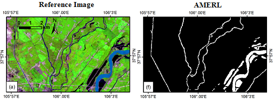
An automated method for extracting rivers and lakes (AMERL) is developed by combining WI with digital image processing techniques to identify water pixels, especially mixed water pixels in shallow or narrow water bodies. In this study, a narrow river is defined as having a width less than or equal to three pixels, because wide rivers (i.e., wider than three pixels) are more likely to contain pure water pixels that are easy to identify by the thresholding method.

2. Study Areas and Data Preparation

2.1. Study Areas

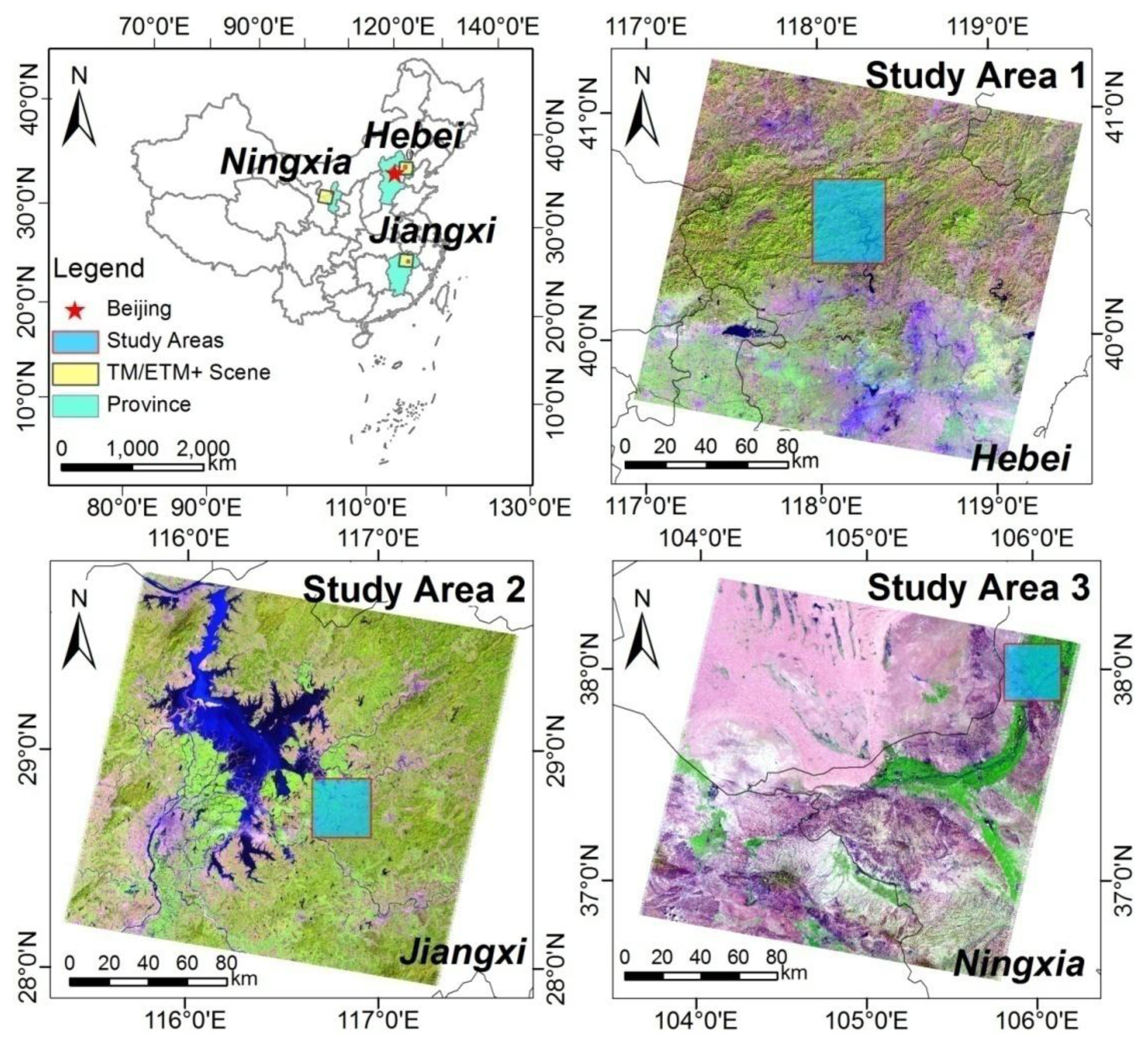
To evaluate the robustness of the new method, three study areas were selected in China with different water body types, climate conditions and land cover (

Table 1. Summary of the study areas and input Landsat images. Alt: altitude.

No	Study Area	Landsat Sensor	Path/Row	Acquisition Date	Image Size (Pixels)	Water Body Type	Climate	Mean Alt. (m)
1	Hebei	TM	p122/r032	23 September 2006	1200 × 1380	Reservoir, river	Temperate, semi-humid	441
2	Jiangxi	ETM+	p121/r040	5 October 2010	1000 × 1000	Reservoir, river	Subtropical, humid	25
3	Ningxia	TM	p130/r034	10 September 2010	1000 × 1000	River, canal	Temperate, semi-arid	1161

). Figure 1 shows the locations and visual characteristics of the three study areas.

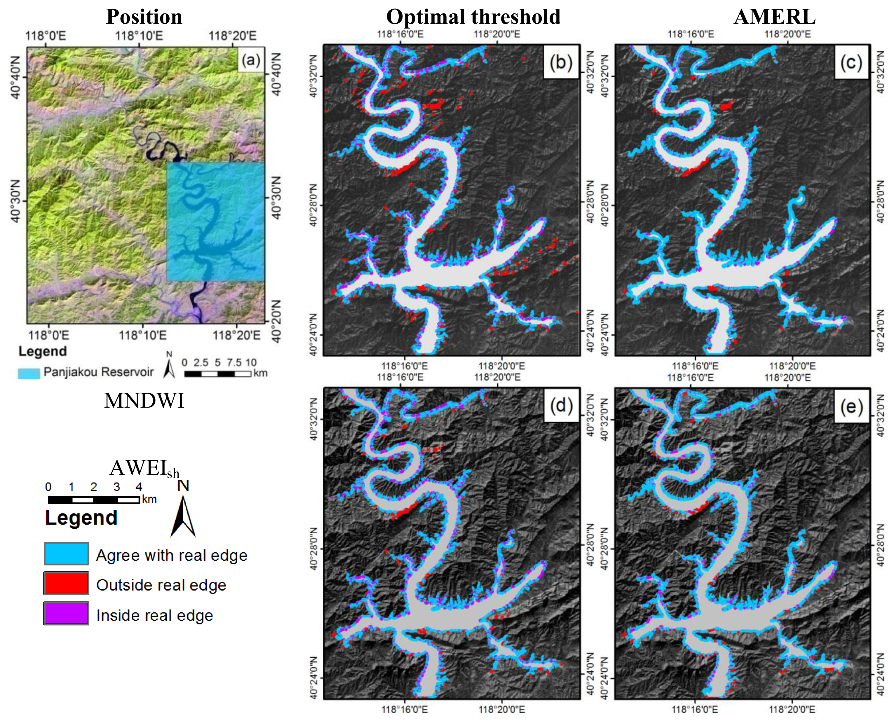
Study Area 1 is located in Hebei Province in northern China and encompasses the Panjiakou Reservoir and five rivers (i.e., Luanhe, Liuhe, Baohe, Heihe and Sahe). Primarily deciduous coniferous forest and shrubs cover the land surface. The area is rugged and mountainous; the elevation ranges from 107 to 1376 m. Therefore, the assessment of the water body extraction method in this area focused on distinguishing between water bodies and mountain shadows.

Study Area 2 is located at the southeast Poyang Lake, which is China’s largest freshwater lake located in Jiangxi Province in southern China. This area has abundant water resources that include eight reservoirs, three rivers (i.e., Leanjiang, Xinjiang and Wannianhe) and several tributaries. The area is primarily flat and is covered with irrigated farmland. Hilly land is located at the southeastern corner of the study area; this portion is covered by evergreen broad-leaved forest. The largest sources of background noise are Yugan County and several villages.

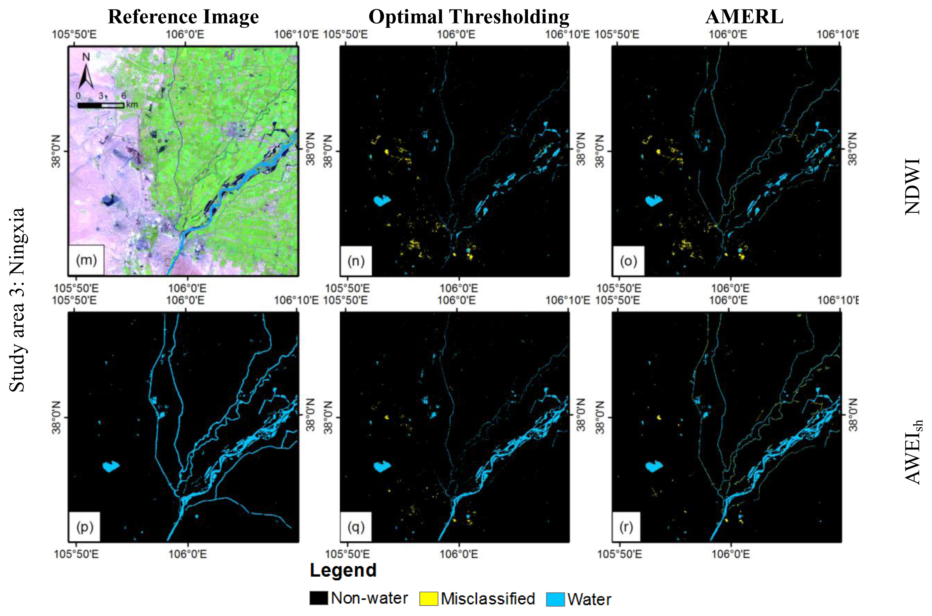
Study Area 3 is located in the Ningxia Hui Autonomous Region of northwestern China. The area is generally flat and is covered primarily by farmland and bare land. The Yellow River, which is the second longest river in China and well known for its turbid water, flows through the study area. This river was selected to test the robustness of the proposed method for turbid water bodies.

2.2. Image Preprocessing

Level 1T Landsat TM/ETM+ images were acquired for this study [3]. These images have been geometrically corrected and in the form of raw DN (digital-number) values. An atmospheric correction was needed to adjust for atmospheric scattering and absorption effects that are caused by ozone, water vapor, aerosols and other particles and for Rayleigh scattering [20]. The Landsat ecosystem disturbance adaptive processing system (LEDAPS, version 1.2.0) algorithm was used to retrieve the surface reflectance data from the DN value [21].

2.3. Reference Data

To provide a basis for comparison, the “true” water bodies were manually digitized from the Landsat images. High-resolution Google Earth™ images were used as a complementary reference to help distinguish confusing water pixels from background noise (e.g., mountain shadows or urban areas).

3. Methods

3.1. Representative Spectral Profiles

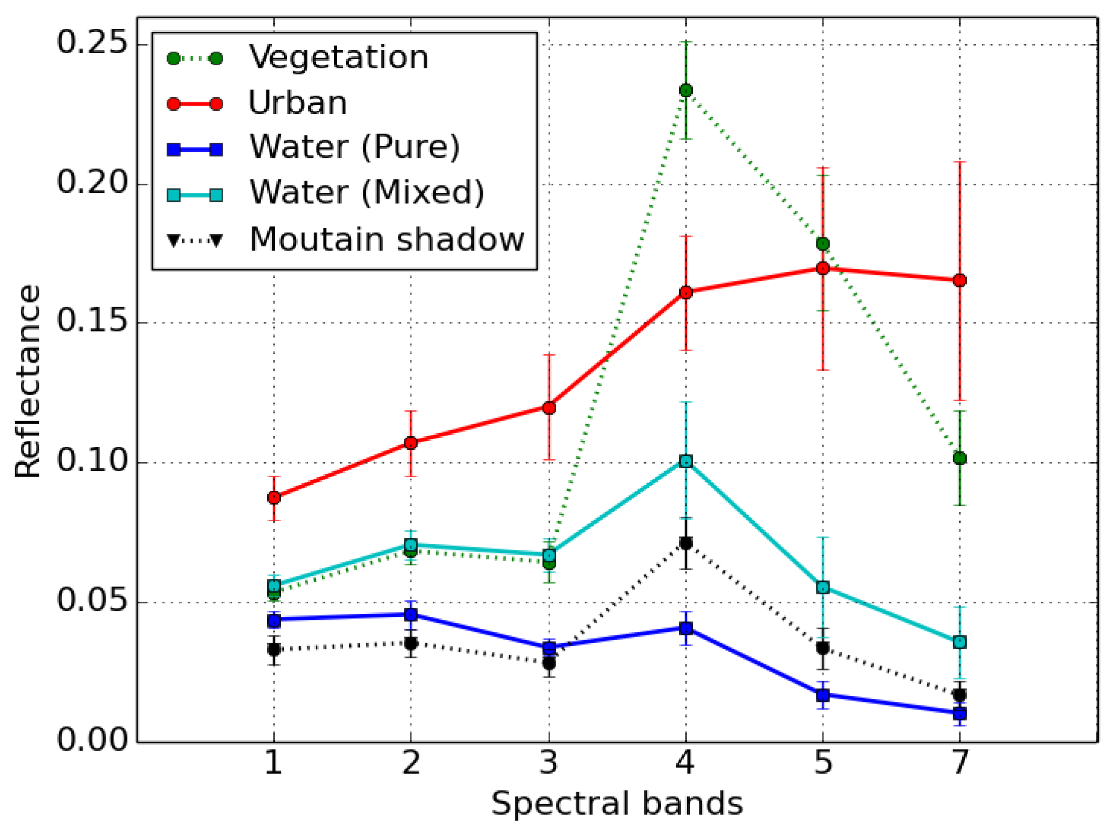
To describe the spectral differences between water bodies and land, 1000 samples were selected to represent the five land cover types (i.e., mixed water, pure water, vegetation, urban and mountain shadow) from the entire scene of the Hebei image, which was used as the source for study Area 1; each category contained 200 samples. The mixed water pixels were sampled from narrow rivers and the edges of lakes or wide rivers. The pure water pixels were selected from the center of reservoirs and lakes, where the water bodies were deep and clear, to guarantee that the pixels contained only water. The other three sample sets were collected based on similar principles to ensure the representativeness of each pixel in the sample sets.

Figure 2 summarizes the reflectance characteristics (mean ± standard deviation) of the samples. The overall spectral reflectance of pure water was lower than that of the vegetation, urban, mountain shadow and mixed water categories [22]. The mixed water reflectance increased with the presence of mud, hydrophytes, suspended sediments, the lake or river bed and/or land (i.e., the riverbank or lake shore). The reflectance pattern for mountain shadows was similar to the pattern for the two water categories, which may lead to confusion between these categories during automated image processing [14].

3.2. Water Index

The WIs are designed to enhance the discrimination between water bodies and land; however, their formulation makes them inherently sensitive to certain types of noise [13].

This study investigates four WIs, including the NDWI (Equation (1)), MNDWI (Equation (2)), AWEI_nsh (Equation (3)) and AWEI_sh (Equation (4)):

$$\text{NDWI}=({\mathrm{\rho }}_2-{\mathrm{\rho }}_4)/({\mathrm{\rho }}_2+{\mathrm{\rho }}_4)$$

(1)

$$\text{MNDWI}=({\mathrm{\rho }}_2-{\mathrm{\rho }}_5)/({\mathrm{\rho }}_2+{\mathrm{\rho }}_5)$$

(2)

$${\text{AWEI}}_{\text{nsh}}=4\times ({\mathrm{\rho }}_2-{\mathrm{\rho }}_5)-(0.25\times {\mathrm{\rho }}_4+2.75\times {\mathrm{\rho }}_7)$$

(3)

$${\text{AWEI}}_{\text{sh}}={\mathrm{\rho }}_1+2.5\times {\mathrm{\rho }}_2-1.5\times ({\mathrm{\rho }}_4+{\mathrm{\rho }}_5)-0.25\times {\mathrm{\rho }}_7$$

(4)

Here, ρ represents the reflectance from the Landsat TM/ETM+ data for Bands 1 (blue), 2 (green), 4 (near-infrared), 5 (SWIR1) and 7 (SWIR2).

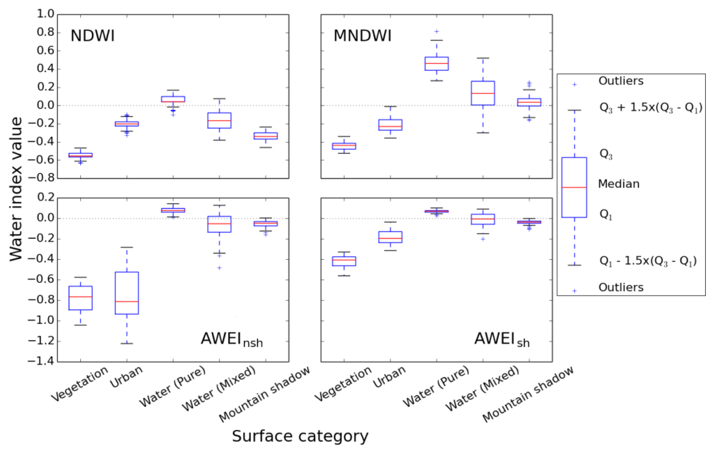
Figure 3 shows the distribution of WI values for the five land cover categories. The pure water pixels exhibit large differences relative to the non-water types for all WIs. The AWEI_nsh is most likely to confuse mixed water pixels with mountain shadow pixels, followed by the MNDWI, AWEI_sh and NDWI. For the NDWI, the mixed water pixels were more often confused with urban pixels than with shadow pixels. In addition, the NDWI and the two AWEIs had smaller ranges of values compared to the MNDWI for water pixels, whereas the AWEI_nsh exhibited the largest ranges of values for non-water pixels.

The characteristics of these distributions are important for developing the processing scheme (Section 3.3) and tuning its parameters (Section 3.6).

3.3. Automated Method for Extracting Rivers and Lakes (AMERL)

As discussed above, pure water pixels can be identified with strict WI thresholds; however, these thresholds may fail to identify mixed water pixels. In contrast, low WI thresholds may capture mixed water pixels; however, these thresholds include more noise.

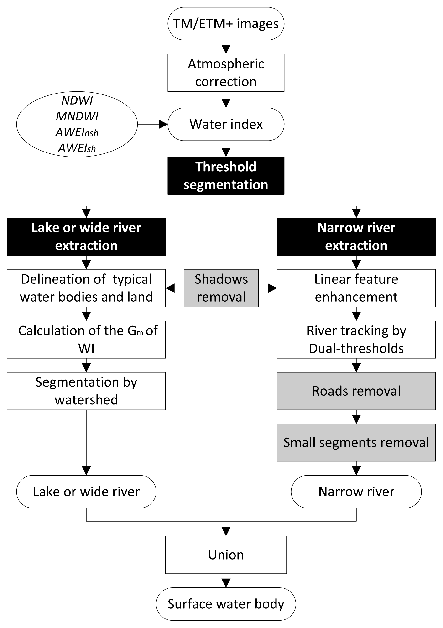
In this paper, an automated method for extracting rivers and lakes (AMERL) was developed to address this issue. Figure 4 illustrates the logic and sequence of operations for this processing scheme. Pure water pixels are extracted using a deliberately selected strict threshold (Thd_pure). This threshold (Thd_pure) is tested for each WI using several training images that have stable characteristics. A watershed segmentation method is then adopted to detect mixed water pixels at the edges of lakes or wide rivers. Moreover, a method based on linear feature enhancement is adopted to detect water pixels from narrow rivers. Lastly, the extracted lakes, wide rivers and narrow rivers are combined to produce the final water body results.

3.4. Lake and Wide River Extraction

The gradient of an image measures its changes in intensity in two aspects: the magnitude of the gradient (G_m) measures the rate at which the intensity changes; the direction of gradient depicts the direction of the maximum increase in intensity [23]. Because the intensity of remote sensing imagery is determined by the land cover spectral reflectance [24], pixels with low G_m represent areas of relatively homogeneous land cover types, whereas pixels with high G_m are associated with areas in which the surrounding land cover may be different.

Although there are differences in the WI values between pure and mixed water pixels, it is reasonable to assume that these differences are smaller than the differences between water and land pixels. Water bodies can be separated from land based on the G_m of WI using the watershed algorithm [23,25].

The original watershed algorithm is sensitive to regional minima and noise, which may lead to the over-segmentation of an image. One solution to this problem is to use markers to specify the allowed regional minima using prior knowledge about the image. The marker is composed of connected pixels in an image. Internal markers focus on objects of interest, while external markers are associated with the background [26]. This marker-controlled watershed segmentation proceeds in three steps.

Step 1: Delineation of typical water bodies and land. Pixels with values greater than Thd_pure are classified as pure water pixels (Section 3.3) and are labeled as internal markers. Pixels with values less than Thd_land are classified as land pixels and are labeled as external markers. Pixels with values between Thd_land and Thd_pure may be land or mixed water pixels; these unmarked pixels are classified in Step 3.

For images of mountainous or hilly regions, shadow pixels must be identified and excluded from internal markers. A simple method for doing this involves thresholding (Thd_shadow; Equation (5) based on the value of Band 2 (green), because Band 2 is more stable than the other bands for differentiating between water bodies and shadows [14]. Shadow reduction methods based on elevation data were not used in this study, because the water areas are highly uncertain in the current existing 30-m resolution digital elevation model (DEM) products, e.g., The Advanced Spaceborne Thermal Emission and Reflection Radiometer (ASTER) [27].

$${\mathrm{\rho }}_2<{\text{Thd}}_{\text{shadow}}$$

(5)

Step 2: Calculation of the G_m of WI. The Sobel operator is used to calculate the G_m of WI. The Sobel operator is a discrete differentiation operator that is used to estimate a digital image gradient. This operator performs better than other gradient operators, such as the Prewitt operator [28].

Step 3: Segmentation by watersheds. The watershed algorithm iteratively expands the internal and external markers [26], and each unmarked pixel is classified as either water body or land. Ultimately, all lakes and wide rivers are extracted in this step.

3.5. Narrow River Extraction

The narrow river extraction method presented here is primarily based on the work of Fischler et al. [29], which focused on the extraction of roads with widths less than or equal to three pixels from remote sensing imagery. Fischler’s method incorporates two steps. First, the method uses the Duda road operator to transform each pixel of an image into a numerical score that indicates the likelihood that the pixel belongs to a linear feature. In the second step, roads are extracted by connecting user-provided seed pixels with a heuristic path-tracking algorithm. This method has also been utilized for river extraction [30]. However, some difficulties prevent this method from being used to automatically map rivers over large areas. In the first step, the Duda road operator is designed to identify straight or smooth curving roads and is not entirely suitable for identifying the numerous and abrupt twists and turns that characterize most natural rivers. In addition, the operator is sensitive to stepwise edges between two homogeneous areas with different image intensity, which may result in several false detections. In the second step, the path-tracking algorithm requires manual intervention that is time consuming.

In this study, the two steps Fischler method was altered in favor of river extraction and added noise reduction procedures as a third step. The three steps of the new narrow river extraction method are introduced below. An example of the results of these steps is shown in Figure 5.

Step 1: Linear feature enhancement (LFE). The objective of LFE is to highlight pixels of linear spatial forms, while suppressing other pixels; thus, the narrow river pixels are easier to track in an LFE image (Figure 5d,e,f) compared with in WIs (Figure 5b,c). To eliminate the aforementioned difficulties that are associated with the Duda road operator, the LFE operator presented in Figure 6 considers only three pixels (the Duda road operator considers nine) at a time to detect the twisted portion of river (meanders). Equation (6) forces the values of pixels that are situated on stepwise edges to become 0:

$${LFE}_i=\{\begin{array}{ll}2a-b-c\hfill & (a>b\mathrm{\hspace{0.17em} }\mathrm{\hspace{0.17em} }\mathrm{\hspace{0.17em} }and\mathrm{\hspace{0.17em} }\mathrm{\hspace{0.17em} }\mathrm{\hspace{0.17em} }a>c)\hfill \\ 0\hfill & (a\le b\mathrm{\hspace{0.17em} }\mathrm{\hspace{0.17em} }\mathrm{\hspace{0.17em} }or\mathrm{\hspace{0.17em} }\mathrm{\hspace{0.17em} }\mathrm{\hspace{0.17em} }a\le c)\hfill \end{array}$$

(6)

Here, i is the index of the four directional operators, and a, b and c are the pixels for a single LFE operator (Figure 6).

The process begins by filtering the image using the four directional operators that are shown in Figure 6 and using Equation (6). Then, the LFE is equivalent to the maximum value of the four directions for each pixel. Lastly, the shadow threshold (Thd_shadow) that was described in Section 3.4 is used to remove mountain shadow pixels.

Step 2: Line tracking. A dual-threshold line tracking algorithm is used in this study to extract rivers from LFE images. This algorithm is based on the classic Canny’s edge-detection method [31]. As part of Canny’s method, dual-threshold line tracking is performed to exclude false edges, while preserving weak edges as much as possible.

During the river segment tracking process, a threshold (Equation (7)) is applied to the WI to exclude non-river areas.

$$\text{WI}>{\text{Thd}}_{\text{river}}$$

(7)

First, pixels with an LFE value that is greater than the higher threshold (Equation (8)) are extracted and classified as river pixels. Then, all pixels with values that are greater than the lower threshold (Equation (8)) and connected to the extracted pixels are also labeled as river pixels:

$$\{\begin{array}{l}{\text{LFE}}_{\text{high}}>0.3\hfill \\ {\text{LFE}}_{\text{low}}>0.2\hfill \end{array}$$

(8)

Step 3: Noise reduction. In this study, mountain shadows, roads and small segments are the primary causes of noise in the water detection results.

Table 2. Characteristics and reduction methods for three important types of noise. LFE, linear feature enhancement.

Noise Type	Cause	Characteristic	Reduction Method
Mountain shadow	Lack of direct sunlight	Low reflectance of each band	Thresholding based on Band 2 (green)
Roads	Introduced by LFE	LFE values that are similar to that of rivers	Thresholding based on LFE using Band 5 (SWIR1)
Small segments	Variety of reasons	Contains only a few pixels	Counting segment sizes to remove small segments

summarizes the characteristics of the noise.

(1)

Mountain shadows: The reduction of mountain shadow pixels is discussed in Section 3.4; it is required for both rivers and lakes extraction. This procedure is turned off by setting Thd_shadow to zero for images with flat topography.

(2)

Roads: Roads against a background of vegetation typically have LFE values that are similar to those of narrow rivers; therefore, roads can be erroneously extracted (Figure 5e). However, the reflectance of roads is higher than that of vegetation in Band 5 (SWIR1) (Figure 5a); thus, the LFE step is performed using Band 5 and then applying a threshold of 0 (Equation (9)) to exclude roads (Figure 5f):

$${\text{LFE}}_{\text{SWIR}1}<0$$

(9)

(3)

Small segments: Small segments are defined as groups of a few connected pixels in the extraction results. These segments are usually misclassifications of mountain ridges and shadows, open spaces, airports, coal yards and other artificial linear facilities or are residuals from the two previous noise reduction steps. These segments are likely to have LFE values that are similar to those of narrow rivers, but are shorter in length or smaller in size. Therefore, they can be eliminated by establishing a threshold for the segment size. The segment size is the number of connected pixels (NP) within a segment. Based on the results of the selected study areas, an empirical threshold of 60 is recommended (Equation (10)):

$$\text{Count\hspace{0.17em}}(\text{number\hspace{0.17em}of\hspace{0.17em}pixels})<60$$

(10)

3.6. Parameter Tuning

Because the AMERL considers comprehensive situations in water body extraction, eight parameters are utilized for different purposes. These parameters were trained on the three study areas and four additional test areas (the test areas are not included in this paper). The values used in study Area 1 are listed in

Table 3. AMERL parameters; the values correspond to those used in study area 1. Thd, threshold. NP, number of pixels.

Group	Threshold	Stability	Value for Each Water Index
			NDWI	MNDWI	AWEInsh	AWEIsh
Water body extraction	Thdpure	Very stable	0	0.3	0.05	0.05
	Thdland		−0.2	−0.2	−0.05	−0.05
	LFEhigh		0.3	0.3	0.6	0.4
	LFElow		0.2	0.2	0.2	0.2
Noise reduction	Thdriver	Relatively stable	−0.4
	NP		60
	Thdshadow	Unstable	0.4
	Thdroads		Not used

. The eight parameters can be categorized into two groups by considering their purpose:

Group 1, used for water body extraction: The values of Thd_pure, Thd_land, LFE_high and LFE_low are dependent on which WI the AMERL is using, because the range of values for a particular land cover varies with each WI (Section 3.2). However, for a given WI, the four parameters are very stable throughout the three study areas and the four test areas.

Group 2, used for noise reduction: The values of Thd_river, NP, Thd_shadow and Thd_roads are independent of the WI. However, this group of parameters is not as stable as those of the first group. The noise reduction parameters can be divided into two sub-groups based on their stability:

• Relatively stable: Thd_river and NP are the same in the three study areas; however, these parameters require additional training in two of the test areas. For example, images of rugged hills contain many non-water linear features; thus, increasing the values of the two parameters may eliminate more noise.
• Unstable: Thd_shadow and Thd_roads typically require manual decisions regarding whether the target image contains the corresponding noise; if the noise is present, a parameter training process should be performed. Otherwise, these parameters should be ignored, because noise reduction methods have the potential to misidentify water bodies as noise. In this study, Thd_shadow is not used in study Areas 2 and 3, whereas Thd_roads is not used in study Area 1.

The accuracy of AMERL in water body extraction is compared with that of an optimal thresholding method. To determine the optimal threshold, a series of thresholds are tested. Each possible threshold generates a water body extraction result; errors are calculated by comparing this result with the reference data. A higher threshold may identify only a few water bodies (i.e., higher omission error); a lower threshold may not only identify many water bodies, but also mistakenly identify land as water bodies (i.e., higher commission error). The optimal threshold corresponds to the minimum total error, which is the sum of the commission and omission errors. In this study, the thresholds for all WIs in this paper are tested using values ranging from −0.1 to 0.1 in increments of 0.01.

4. Results and Discussion

The overall water body extraction performance was first tested via visual inspection and a pixel-by-pixel assessment of the images. Subsequently, detailed evaluations of the results were conducted using several metrics to assess the performance of the proposed method in identifying mixed water pixels at the edges of lakes or wide rivers and in narrow rivers.

4.1. Overall Water Body Mapping Performance

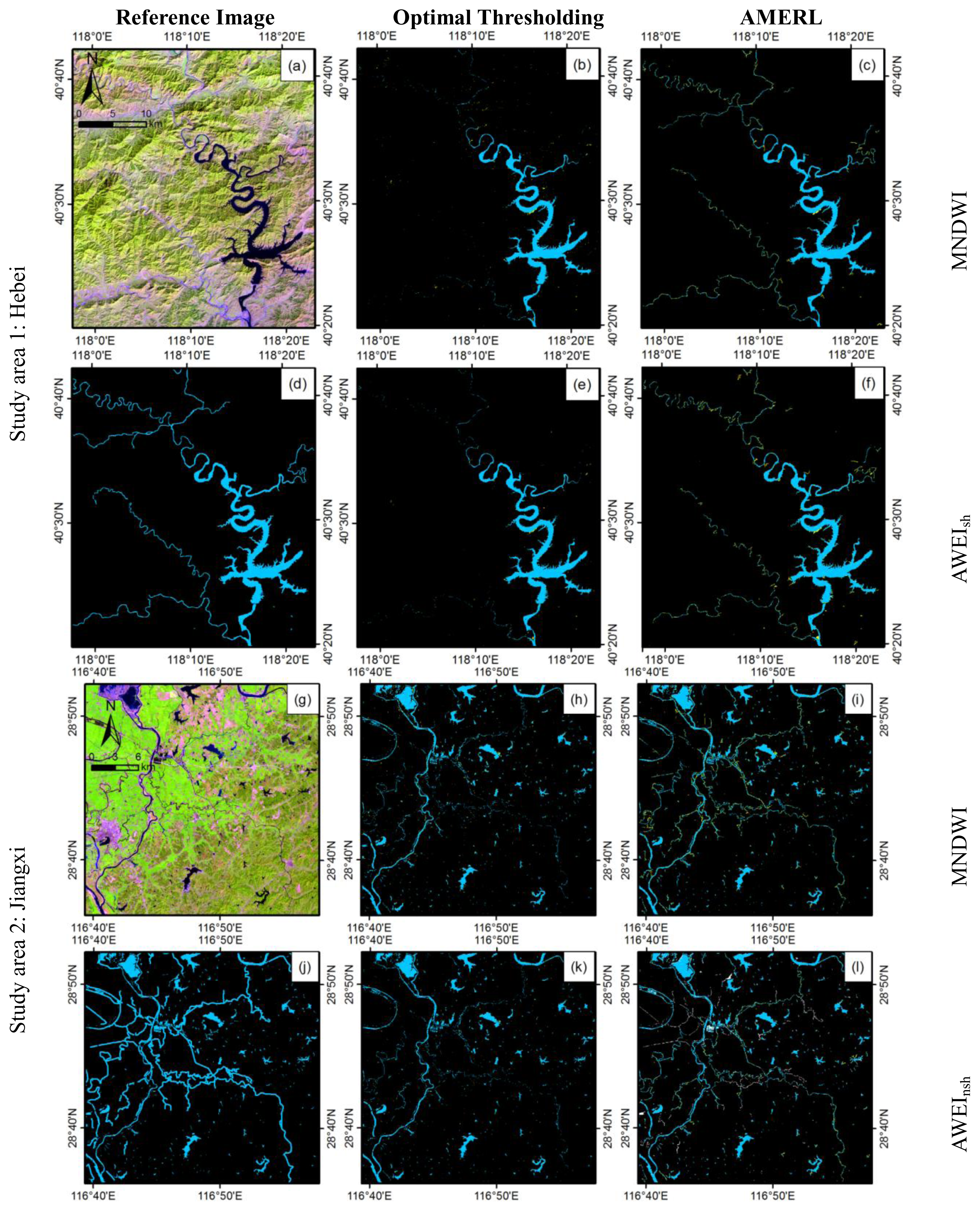
The performance of the AMERL was compared with the optimal thresholding results for each of the four WIs in the three study areas (

Table 4. Accuracies of water body extraction using the optimal thresholding method and the AMERL for the four water indices.

		Accuracy (%)
Study Area	Water Index	Method	User	Producer	Kappa	Total Error (%)
Hebei	NDWI	Thd = −0.1	98.71	79.58	0.9909	21.71
		AMERL	92.50	91.91	0.9934	15.59
	MNDWI	Thd = 0.06	96.67	84.50	0.9922	18.83
		AMERL	92.68	95.78	0.9950	11.54
	AWEInsh	Thd = −0.03	98.16	80.59	0.9912	21.25
		AMERL	91.42	89.19	0.9919	19.39
	AWEIsh	Thd = −0.02	97.75	85.31	0.9930	16.94
		AMERL	89.16	95.87	0.9933	14.97
Jiangxi	NDWI	Thd = −0.1	98.82	57.03	0.9726	44.15
		AMERL	93.07	72.72	0.9795	34.20
	MNDWI	Thd = −0.05	93.01	84.68	0.9864	22.31
		AMERL	85.42	93.25	0.9858	21.33
	AWEInsh	Thd = −0.1	96.95	80.58	0.9862	22.47
		AMERL	93.01	86.16	0.9872	20.83
	AWEIsh	Thd = −0.1	93.25	83.62	0.9859	23.13
		AMERL	85.06	90.95	0.9843	23.99
Ningxia	NDWI	Thd = −0.1	76.67	42.00	0.9765	81.33
		AMERL	77.27	54.24	0.9795	68.49
	MNDWI	Thd = −0.03	93.90	85.40	0.9933	20.70
		AMERL	91.65	90.35	0.9941	18.00
	AWEInsh	Thd = −0.1	99.10	69.29	0.9896	31.62
		AMERL	95.61	75.98	0.9909	28.41
	AWEIsh	Thd = −0.05	93.59	75.64	0.9902	30.77
		AMERL	88.44	91.01	0.9931	20.54

); however, to display the results concisely, only two representative WIs were demonstrated for each study area (Figure 7).

A visual inspection indicates that the AMERL successfully extracted most of the narrow rivers in all of the study areas, whereas the optimal thresholding method extracted only small portions of these narrow rivers. However, regarding most of the lakes or wide rivers, there was little difference between the optimal thresholding method and the AMERL or among the four WIs. This similarity arises because the optimal thresholding method is sufficient to extract pure water pixels in this water body type. However, the extraction of wide river pixels, primarily in the Yellow River within study Area 3, using the NDWI is an exception. Due to the very high sediment load, the reflectance of the Yellow River in the near-infrared band is larger than in the green band; thus, the NDWI values in the wide river were smaller than the value of several bare land pixels. Both the AMERL and the optimal thresholding method failed to extract most of the pixels in the Yellow River using the NDWI in study Area 3.

Table 4 provides a pixel-by-pixel analysis of the classification accuracies based on four metrics: the user’s and producer’s accuracy, the kappa coefficient, and the total error. In comparison with the optimal thresholding method, the total error of the AMERL decreased by 1% to 12.8% for eleven of the twelve tests (i.e., the tests of four WIs in three study areas). The one exception was the AWEI_sh in Jiangxi (i.e., study area 2), which had a slightly higher total error using the AMERL. The reason for this discrepancy is discussed in Section 4.3. The improvements of water body extraction accuracies are insignificant regarding these metrics, because AMERL’s main objective is to enhance the ability to identify the mixed water pixels; however, the mixed water pixels are less than pure water pixels. Thus, additional metrics are required for evaluating the extraction results that focus on the mixed water pixels, including three metrics for them on edges of lakes and wide rivers (Section 4.2) and three metrics for them on narrow rivers (Section 4.3).

Among the WIs, the optimal threshold values are varied with each study area (Table 4); however, the AMERL uses the same water extraction parameters for all three study areas. It is only required to specify the noise reduction parameters, Thd_shadow and Thd_roads. As AMERL’s accuracies are not less than the optimal thresholding method, it is reasonable to believe that the parameter tuning is easier in the AMERL than the thresholding method.

4.2. Accuracy of the Edge Positions for the Extracted Lakes and Wide Rivers

The accuracy of the extraction of lakes and wide rivers was assessed using a subset of the images for study Area 1 (Figure 8). The image size is 500 × 595 pixels and is focused on the Panjiakou Reservoir in an area without rivers. The results using the optimal thresholding method and the AMERL were compared for the four WIs; however, Figure 8 only shows the results for two representative WIs.

To further evaluate the identification of mixed pixels at the edges of lakes and wide rivers, the boundary extraction method was used to identify the edges of the extracted water bodies and the manually interpreted reference images. Boundary extraction is a simple morphological image processing algorithm that extracts the outermost pixels of features from a binary image [23]. Three metrics were applied to evaluate the results from different perspectives:

$$\text{A}={\text{N}}_{\text{t}}/{\text{N}}_{\text{R}}\times 100\%$$

(11)

$${\text{E}}_{\text{C}}={\text{N}}_{\text{C}}/{\text{N}}_{\text{R}}\times 100\%$$

(12)

$${\text{E}}_{\text{O}}={\text{N}}_{\text{O}}/{\text{N}}_{\text{R}}\times 100\%$$

(13)

such that A + E_C + E_O = 100%. Here, A is the accuracy of the edge position, E represents the edge position error frequency (C for commission and O for omission), N_R is the number of edge pixels in the reference image, N_t is the total number of extracted edge pixels in the reference image, N_C is the number of extracted edge pixels that lie outside the reference water bodies (i.e., the number of commission errors) and N_O is the number of extracted edge pixels that lie inside the reference water bodies and that are not directly adjacent to the actual edge (i.e., omission errors).

Table 5. Edge extraction accuracy assessment for Panjiakou Reservoir using the default thresholding method (Thd), the optimal thresholding method (Thd_opti) and the AMERL. The image used in this analysis was clipped from the image for study Area 1 and is shown in Figure 8. E: errors (C, commission; O, omission); A: accuracy of edge detection.

Water index	Method	EC (%)	EO (%)	A (%)
NDWI	Thd = −0.1	4.39	45.79	49.82
	Thdopti = −0.19	15.69	16.52	67.79
	AMERL	8.00	17.87	74.14
MNDWI	Thd = 0	17.31	17.94	64.75
	Thdopti = 0.02	13.97	21.15	64.88
	AMERL	6.66	11.23	82.11
AWEInsh	Thd = 0	1.69	58.22	40.09
	Thdopti = −0.05	9.19	35.94	54.88
	AMERL	9.60	15.30	75.10
AWEIsh	Thd = 0	4.32	32.52	63.16
	Thdopti = −0.02	9.83	20.64	69.53
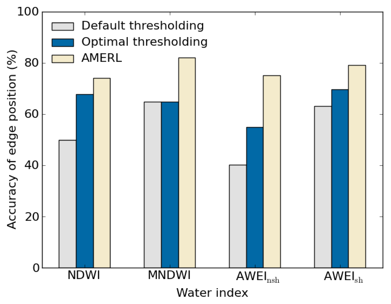
	AMERL	10.47	10.41	79.11

summarizes the edge extraction accuracy for Panjiakou Reservoir using the default thresholding method (non-optimized), the optimal thresholding method (Thd_opti) and the AMERL. The default thresholding method exhibits either high commission or omission errors in the water body results; therefore, this approach had the lowest accuracy among the three methods. For the optimal thresholding method, the highest A was achieved with the AWEI_sh, followed by the NDWI, MNDWI and AWEI_nsh. However, using the AMERL, the highest A was achieved with the MNDWI, followed by the AWEI_sh, AWEI_nsh and NDWI. The largest improvements relative to the optimal thresholding method using the AMERL were achieved by the AWEI_nsh (20.2%) and MNDWI (17.2%); the AWEI_sh (9.6%) and NDWI (6.4%) exhibited smaller improvements (Figure 9). The reason for this result is that the AWEI_nsh and MNDWI are more vulnerable to shadow pixels than the AWEI_sh and NDWI; thus, the extra shadow reduction procedure in the AMERL provides a larger improvement.

However, there is an area that is situated 260 m above the Panjiakou Reservoir (measured using Google Earth) and located in the central region of the reservoir (Figure 8). This area casts a shadow on the water body and bank. None of the methods used in this study were able to accurately identify the actual edge of the reservoir in this area. Although this problem did not introduce large errors in the overall water body extraction, it could be eliminated in future research by introducing a digital elevation model (DEM) with a sufficient spatial resolution and high data quality to accurately identify shadow pixels.

4.3. Completeness of the Narrow River Extraction

Metrics that are based on feature length are often used to assess the results of extracting linear features, such as roads or narrow rivers, instead of a pixel-by-pixel comparison. To provide a detailed analysis of the narrow river extraction results, three metrics were chosen [32]:

$$\text{completeness}={\text{L}}_{\text{m}}/{\text{L}}_{\text{r}}\times 100\%$$

(14)

$$\text{correctness}={\text{L}}_{\text{m}}/{\text{L}}_{\text{e}}\times 100\%$$

(15)

$$\text{quality}={\text{L}}_{\text{m}}/({\text{L}}_{\text{u}}+{\text{L}}_{\text{e}})\times 100\%$$

(16)

where L_m is the total length of the extracted river that matches the river in the reference image, L_r is the total length of the reference river, L_e is the total length of the extracted river and L_u is the total length of over- or under-extracted rivers that are unmatched with the reference rivers.

Table 6. Evaluation of the optimal thresholding method and the AMERL results.

Completeness (%)
Study Area	Water Index	Optimal Threshold	AMERL	Correctness (%)	Quality (%)
Hebei	NDWI	15.07	72.75	90.66	67.68
	MNDWI	31.07	84.85	90.23	77.71
	AWEInsh	12.47	50.38	76.39	43.59
	AWEIsh	19.00	74.94	82.96	64.94
Jiangxi	NDWI	9.44	58.53	98.67	58.07
	MNDWI	54.56	84.93	95.70	81.81
	AWEInsh	34.35	67.66	99.05	67.22
	AWEIsh	23.87	82.56	97.06	80.55
Ningxia	NDWI	41.80	75.22	96.69	73.34
	MNDWI	56.30	89.71	95.60	86.15
	AWEInsh	26.06	49.48	98.16	49.02
	AWEIsh	35.94	89.42	92.83	83.65

summarizes these values for the river extraction procedure.

Because the results extracted using the optimal thresholding method may contain large amounts of noise caused by urban areas and shadows that cannot be measured in terms of length, the optimal thresholding method is only compared with the AMERL using the completeness metric (Figure 10); however, the correctness and quality metrics are used to assess the results of the AMERL.

There are many mountain ridges and shadow areas in study Area 1: these regions may have a linear form in remote sensing imagery that can be enhanced during the linear feature enhancement procedure. Figure 7b (MNDWI) and Figure 7e (AWEI_sh) show that the optimal thresholding method extracted only a few fragments of the Luanhe, Liuhe and Sahe Rivers and completely missed the other two rivers. Figure 7c shows that the AMERL using the MNDWI extracted all five rivers and some of their tributaries; although there were a few gaps in the results. The AMERL using the AWEI_sh also extracted the five rivers; however, it failed to identify the tributaries. Table 6 shows that the optimal thresholding method exhibited poor completeness of river extraction for the four WIs (completeness_thd). The highest completeness among the optimal thresholding methods or the AMERL was for the MNDWI; the AWEI_nsh resulted in the lowest completeness. The highest completeness (MNDWI) was substantially increased with the AMERL (to 84.8%). Even the AMERL’s lowest completeness (50.4% for the AWEI_nsh) was higher than the highest completeness from the optimal thresholding method (31.1% for the MNDWI).

Study Area 2 is covered by dense vegetation and abundant water bodies. Figure 7e,f,h,i shows that the wide Leanjiang and Xinjiang Rivers were successfully extracted by the four WIs using both methods. The main difference occurred in narrow regions of the Wannianhe River and tributaries between the Leanjiang and Xinjiang Rivers. Table 6 shows that with the optimal thresholding method, the highest completeness for this area was achieved by the MNDWI (54.6%); the lowest completeness was achieved by the NDWI for both methods. The MNDWI also resulted in the highest completeness in the AMERL (84.9%); the lowest completeness in the AMERL (58.5%) was greater than the completeness for any WIs using the optimal thresholding method.

Study Area 3 contains six canals near the Yellow River; its primary noise sources are several roads near Qingtongxia City. Table 6 indicates that the MNDWI resulted in the highest completeness for both methods. The AWEI_sh performed as well as the MNDWI in the AMERL, although no mountain shadows were present in this area. The NDWI failed to identify the Yellow River; however, it extracted more canals than the AWEI_nsh, because the canals contained less sediment. Most roads were eliminated by the noise reduction process, while a few road segments that intersected the rivers remained; the line segment reduction process was unable to remove this noise.

According to the completeness metric, all WIs have the potential to improve narrow river extraction using the AMERL. Moreover, the MNDWI and AWEI_sh outperformed the NDWI and AWEI_nsh in all tests. The AMERL results were further assessed for correctness and quality (Table 6). With the exceptions of the two AWEIs in study Area 1, the correctness values for the other ten tests were greater than 90%, implying that the overestimation of narrow rivers by the proposed method is small. The quality may be reduced by either an overestimation or an underestimation of narrow rivers. The high correctness performed in this study suggests that underestimation has a larger effect on reducing quality. This finding is exemplified using the NDWI and the AWEI_nsh. Because study Area 2 is covered by dense vegetation, the narrow river pixels usually contain a mixture of water bodies and vegetation; the NDWI is inefficient at identifying this pixel type. The AWEI_nsh in study Areas 1 and 3 also exhibited a notable underestimation due to the misclassification of most of the narrow rivers.

The AMERL is designed to improve the WIs for the identifying of rivers with widths that are less than or equal to three pixels. However, portions of the extracted narrow rivers may wider than their actual width. The third column of images in Figure 7 shows a few misclassified pixels (yellow) along the narrow rivers, especially in study Area 2. Therefore, the user’s accuracy (Table 4) decreased for most of the WIs, whereas the producer’s accuracy (Table 4) and the completeness values (Table 6) increased. This pattern occurs because the WI value of mixed land pixels is higher than that of surrounding pure land pixels, even though land, not water body, is the dominant category. These pixels were connected to narrow river pixels and may also have been incorrectly extracted. To identify these pixels with sub-pixel precision, it would be necessary to analyze the proportions of land and water bodies in the mixed pixels and the surface type of the land, which is beyond the scope of this study. However, for simple applications, such as vectorizing rivers, the “thinning” morphological operator [33] may help to properly reduce the width of the extracted rivers.

The river extraction method may fail if a river is too narrow (i.e., less than one pixel), which means there is a minimum width below which the AMERL may provide unstable results. In this study, the width limitation in six canals of different widths in study Area 3 was tested using Google Earth™ by measuring the width of the canals where the river extraction method failed. In this analysis, the AMERL was used with the better performing WIs, i.e., the MNDWI and AWEI_sh. For the three canals that were wider than one pixel, the AMERL extracted the entire length of the canals with no failures. For the two canals with widths that ranged from 20 to 40 m (2/3 to 4/3 of a pixel), the extraction failed at three locations for each WI. The width of the three locations ranged from 17 m to 25 m, which means that the narrow river extraction method was unstable for rivers with a width of 25 m or less in the TM/ETM+ images. The canal at the bottom right of Figure 7p was approximately 12 m-wide; none of the WIs extracted even a small portion of this canal.

5. Conclusions

There are several difficulties associated with water body extraction from satellite imagery using water indices (WIs) that are based on the thresholding method, including: (1) inefficient identification of mixed water pixels; (2) confusion of water bodies with background noise; and (3) variations in the optimal water extraction threshold that depend on the characteristics of an individual scene. Considering that mixed water pixels usually appear in narrow rivers or along the edge of lakes or wide rivers, the automated method for extracting rivers and lakes (AMERL) is proposed for extracting mixed water pixels by considering not only their spectral characteristics, but also their topological connections. A series of processes are introduced to filter out noise caused by shadows, roads and small segments by considering both their spatial and spectral characteristics. The threshold optimization procedure is also simplified using AMERL.

The ability of the new method to improve the extraction of water bodies was tested based on four WIs calculated for Landsat TM (Thematic Mapper) and ETM+ (Enhanced Thematic Mapper Plus) imagery over three study areas in China. The AMERL outperformed the optimal thresholding method for most WIs in all study areas. The AMERL substantially improved the completeness of narrow rivers extraction for all four WIs. However, the modified normalized-difference water index (MNDWI) [12] and automated water extraction index (AWEI_sh, with shadow presence) [14] exhibited a larger improvement than the normalized-difference water index (NDWI) [11] and AWEI_nsh (without shadow presence) [14] in each of the three study areas. The proposed method can be further improved to take advantage of the high-resolution digital elevation model (DEM) for shadow reduction. Further applications are required to assess the robustness of the method on imagery from other sensors and other areas of the world.

References

1. Langbein, W.B.; Iseri, K.T. General Introduction and Hydrologic Definitions; US Government Printing Office: Washington, DC, USA, 1960. [Google Scholar]
2. National Research Council, Integrating Multiscale Observations of U.S. Waters; The National Academies Press: Washington, DC, USA, 2008.
3. U.S. Geological Survey. USGS Global Visualization Viewer. Available online: http://glovis.usgs.gov (accessed on 19 March 2014).
4. Goodwin, N.R.; Collett, L.J.; Denham, R.J.; Flood, N.; Tindall, D. Cloud and cloud shadow screening across Queensland, Australia: An automated method for Landsat TM/ETM+ time series. Remote Sens. Environ 2013, 134, 50–65. [Google Scholar]
5. Verpoorter, C.; Kutser, T.; Tranvik, L. Automated mapping of water bodies using Landsat multispectral data. Limnol. Oceanogr 2012, 10, 1037–1050. [Google Scholar]
6. Rundquist, D.C.; Lawson, M.P.; Queen, L.P.; Cerveny, R.S. The relationship between summer-season rainfall events and lake-surface area. J. Am. Water Resour. Assoc 1987, 23, 493–508. [Google Scholar]
7. Lu, D.; Weng, Q. A survey of image classification methods and techniques for improving classification performance. Int. J. Remote Sens 2007, 28, 823–870. [Google Scholar]
8. Otukei, J.; Blaschke, T. Land cover change assessment using decision trees, support vector machines and maximum likelihood classification algorithms. Int. J. Appl. Earth Obs. Geoinf 2010, 12, S27–S31. [Google Scholar]
9. Frazier, P.S.; Page, K.J. Water body detection and delineation with Landsat TM data. Photogramm. Eng. Remote Sens 2000, 66, 1461–1468. [Google Scholar]
10. Townshend, J.R.; Justice, C. Analysis of the dynamics of African vegetation using the normalized difference vegetation index. Int. J. Remote Sens 1986, 7, 1435–1445. [Google Scholar]
11. McFeeters, S. The use of the Normalized Difference Water Index (NDWI) in the delineation of open water features. Int. J. Remote Sens 1996, 17, 1425–1432. [Google Scholar]
12. Xu, H. Modification of normalised difference water index (NDWI) to enhance open water features in remotely sensed imagery. Int. J. Remote Sens 2006, 27, 3025–3033. [Google Scholar]
13. Ji, L.; Zhang, L.; Wylie, B. Analysis of dynamic thresholds for the normalized difference water index. Photogramm. Eng. Remote Sens 2009, 75, 1307–1317. [Google Scholar]
14. Feyisa, G.L.; Meilby, H.; Fensholt, R.; Proud, S.R. Automated Water Extraction Index: A new technique for surface water mapping using Landsat imagery. Remote Sens. Environ 2014, 140, 23–35. [Google Scholar]
15. Jiang, Z.; Qi, J.; Su, S.; Zhang, Z.; Wu, J. Water body delineation using index composition and HIS transformation. Int. J. Remote Sens 2012, 33, 3402–3421. [Google Scholar]
16. Lira, J. Segmentation and morphology of open water bodies from multispectral images. Int. J. Remote Sens 2006, 27, 4015–4038. [Google Scholar]
17. Lu, S.; Wu, B.; Yan, N.; Wang, H. Water body mapping method with HJ-1A/B satellite imagery. Int. J. Appl. Earth Obs. Geoinf 2011, 13, 428–434. [Google Scholar]
18. Fisher, A.; Danaher, T. A water index for SPOT5 HRG Satellite imagery, New South Wales, Australia, determined by linear discriminant analysis. Remote Sens 2013, 5, 5907–5925. [Google Scholar]
19. Sivanpillai, R.; Miller, S.N. Improvements in mapping water bodies using ASTER data. Ecol. Inform 2010, 5, 73–78. [Google Scholar]
20. Maiersperger, T.; Scaramuzza, P.; Leigh, L.; Shrestha, S.; Gallo, K.; Jenkerson, C.; Dwyer, J. Characterizing LEDAPS surface reflectance products by comparisons with AERONET, field spectrometer, and MODIS data. Remote Sens. Environ 2013, 136, 1–13. [Google Scholar]
21. Feng, M.; Sexton, J.O.; Huang, C.; Masek, J.G.; Vermote, E.F.; Gao, F.; Narasimhan, R.; Channan, S.; Wolfe, R.E.; Townshend, J.R. Global surface reflectance products from Landsat: Assessment using coincident MODIS observations. Remote Sens. Environ 2013, 134, 276–293. [Google Scholar]
22. Davis, S.M.; Landgrebe, D.A.; Phillips, T.L.; Swain, P.H.; Hoffer, R.M.; Lindenlaub, J.C.; Silva, L.F. Remote Sensing: The Quantitative Approach; McGraw-Hill International Book Co: New York, NY, USA, 1978. [Google Scholar]
23. Gonzalez, R.C.; Woods, R.E.; Eddins, S.L. Digital Image Processing Using MATLAB; Gatesmark Publishing Knoxville: Knoxville, TN, USA, 2009. [Google Scholar]
24. Sanderson, R. Introduction to Remote Sensing. Available online: http://faculty.kfupm.edu.sa/crp/bramadan/crp514/readings/7%20-%20Introd_Remote_Sensing_Dr_Sanderson_New_Mexico_State_Univ_38Pages.pdf (accessed on 14 February 2014).
25. Meyer, F. The Watershed Concept and Its Use in Segmentation: A Brief History. Available online: http://arxiv.org/pdf/1202.0216.pdf (accessed on 14 February 2014).
26. Soille, P.J.; Ansoult, M.M. Automated basin delineation from digital elevation models using mathematical morphology. Signal. Process 1990, 20, 171–182. [Google Scholar]
27. ASTER GDEM Validation Team. ASTER Global DEM Validation. Summary Report. 2009. Available online: https://lpdaac.usgs.gov/sites/default/files/public/aster/docs/ASTER_GDEM_Validation_Summary_Report.pdf (accessed on 10 February 2014).
28. Wikipedia Contributors. Sobel Operator. Available online: http://en.wikipedia.org/wiki/Sobel_operator (accessed on 19 March 2014).
29. Fischler, M.A.; Tenenbaum, J.M.; Wolf, H.C. Detection of roads and linear structures in low-resolution aerial imagery using a multisource knowledge integration technique. Comp. Graph. Image Proc 1981, 15, 201–223. [Google Scholar]
30. Dillabaugh, C.R.; Niemann, K.O.; Richardson, D.E. Semi-automated extraction of rivers from digital imagery. GeoInformatica 2002, 6, 263–284. [Google Scholar]
31. Canny, J. A computational approach to edge detection. IEEE Trans. Pattern Anal. Mach. Intell 1986, PAMI-8, 679–698. [Google Scholar]
32. Hu, J.; Razdan, A.; Femiani, J.C.; Cui, M.; Wonka, P. Road network extraction and intersection detection from aerial images by tracking road footprints. IEEE Trans. Geosci. Remote Sens 2007, 45, 4144–4157. [Google Scholar]
33. Lam, L.; Lee, S.-W.; Suen, C.Y. Thinning methodologies—A comprehensive survey. IEEE Trans. Pattern Anal. Mach. Intell 1992, 14, 869–885. [Google Scholar]
Figure 1. Locations of the three study areas in China. Study Area 1 includes the Panjiakou Reservoir in Hebei Province. Study Area 2 includes Yugan County in Jiangxi Province. Study Area 3 includes the Qingtongxia Reservoir in the Ningxia Hui Autonomous Region.
Remotesensing 06 05067f1
Figure 2. Means and standard deviations of surface reflectance in the five land cover types.
Remotesensing 06 05067f2
Figure 3. Water index (WI) value distributions for mixed water, pure water, vegetation, urban and mountain shadow surface categories. In the box and whisker plots, the second, third and fourth horizontal lines from the bottom represent the first quartile (Q1), median and third quartile (Q3), respectively. The bottom and top lines from the bottom represent Q1—1.5 × (Q3 − Q1) and Q3 + 1.5 × (Q3 − Q1), respectively. The crosses (+) indicate outliers.
Remotesensing 06 05067f3
Figure 4. The automated method for extracting rivers and lakes (AMERL) scheme for extracting rivers and lakes from Landsat imagery. NDWI, normalized-difference water index; MNDWI, modified NDWI; AWEI, automated water extraction index.
Remotesensing 06 05067f4
Figure 5. Results of several important steps in the AMERL. The images depict a portion of study area 3. (a) TM 543 band false-color image; (b) MNDWI; (c) results of the optimal thresholding method for comparison; (d) linear feature enhancement (LFE); (e) results of the AMERL without road (red-asterisk) reduction; (f) final results of the AMERL.
Remotesensing 06 05067f5
Figure 6. Four directional linear feature enhancement operators.
Remotesensing 06 05067f6
Figure 7. Comparison of reference images (left) with the water body mapping results using the optimal thresholding method (middle) and the AMERL (right). The images are labeled with the name of the study area (to the left of the images) and the WI used in the extraction (to the right of the images). Note that for demonstration purposes, the results of only two WIs are provided for each study area. The reference images are TM/ETM+ 543 band false-color images (a,g,m) and manually interpreted results images (d,j,p). Note that the manually interpreted results (d,j,p) have been vectorized in order to exhibit the spatial distributions of the narrow rivers more clearly.
Remotesensing 06 05067f7aRemotesensing 06 05067f7b
Figure 8. Comparison of reference images (left) the Panjiakou Reservoir extraction results using the optimal thresholding method (middle) and the AMERL (right).
Remotesensing 06 05067f8
Figure 9. The edge extraction accuracy for Panjiakou Reservoir using the three methods in study Area 1.
Remotesensing 06 05067f9
Figure 10. Improvement in completeness for the AMERL compared with the optimal thresholding method in twelve tests (i.e., four WIs and three study areas). The three study areas are Hebei, Jiangxi and Ningxia. The symbols N, M, Ansh and Ash represent the NDWI, MNDWI, AWEInsh and AWEIsh, respectively.
Remotesensing 06 05067f10