Evaluating the Effect of Different Wheat Rust Disease Symptoms on Vegetation Indices Using Hyperspectral Measurements

Abstract

Spectral Vegetation Indices (SVIs) have been widely used to indirectly detect plant diseases. The aim of this research is to evaluate the effect of different disease symptoms on SVIs and introduce suitable SVIs to detect rust disease. Wheat leaf rust is one of the prevalent diseases and has different symptoms including yellow, orange, dark brown, and dry areas. The reflectance spectrum data for healthy and infected leaves were collected using a spectroradiometer in the 450 to 1000 nm range. The ratio of the disease-affected area to the total leaf area and the proportion of each disease symptoms were obtained using RGB digital images. As the disease severity increases, so does the scattering of all SVI values. The indices were categorized into three groups based on their accuracies in disease detection. A few SVIs showed an accuracy of more than 60% in classification. In the first group, NBNDVI, NDVI, PRI, GI, and RVSI showed the highest amount of classification accuracy. The second and third groups showed classification accuracies of about 20% and 40% respectively. Results show that few indices have the ability to indirectly detect plant disease.

1. Introduction

Spectral data in different scales including leaf, canopy, and remote sensing have been widely used in precision farming [1–4]. In recent years, researchers have studied various Spectral Vegetation Indices (SVIs) to detect different vegetation diseases [4–6]. Efficient use of spectral data to detect diseases depends on aim and application. Only a few ranges of the spectrum are useful. The regions from 400 to 700 and 700 to 1100 nm are mainly influenced by pigments, structure, and water content [7].

The effect of a disease on the pigments and structure of a plant and the change in its spectral response makes SVIs very valuable for disease evaluation [8].

The indices designed and based on several wavelengths are able to detect and identify various substances in vegetation, such as Chlorophyll, Antocynin, Nitrogen, and Water [9,10]. Some investigations show the potential of SVIs for disease detection. Mahlein et al. and Rump et al. showed the effect of disease symptoms on recorded spectra [11,12].

Wheat has three types of rust disease called yellow rust, leaf rust, and stem rust. Leaf rust has the highest abundance compared with the other two types, making it have more priority for further assessment. Each year, it causes so much damage. Leaf rust is caused by the Puccinia triticina fungus and consists of different symptoms [13]. These symptoms begin by manifesting themselves in yellow, orange, and dark brown colors. Finally, the disease symptoms end in a dry leaf. Furthermore, different symptoms of the leaf rust are simultaneously observed in various areas of the leaf [14].

In a large number of investigations, vegetation indices are employed to study wheat rust in the leaf and canopy models. In 1991, Hansen studied the effect of yellow rust on crop yield [15]. Results showed that hyperspectral data have the potential to detect changes in crop productivity made by rust with a correlation higher than 0.9. In another study in 2007, Wenjiangn et al. investigated the relationship between wheat yellow rust and the Photochemical Reflectance Index (PRI) [16]. This index was found to detect yellow color variations with a correlation coefficient of (r² > 0.9). Meanwhile, spectrographical data in the 463~895 nm waveband with 19 bands using the neural network algorithm are able to detect the yellow rust disease with a precision of 0.99. Regarding the fact that the effect of the lack of nitrogen is similar, the detection of the wheat yellow rust in situations of nitrogen scarcity was studied by Zhang et al. using hyperspectral data [4]. Results showed that wheat yellow rust can be detected when nitrogen is lacking.

Yellow rust is seen as narrow yellow strips parallel to nervures on the leaf while leaf rust appears as spots with various colors and patterns [17]. However, research on the leaf rust has been limited compared to the yellow rust.

Devades et al. used 10 SVIs in the visible and infrared region to detect different types of rust at the leaf level [18]. In this research, none of the indices was able to detect and discriminate the three types of rust. However, the Anthocyanin Reflectance Index (ARI) can be used to detect the yellow rust while the Transformed chlorophyll Absorption and Reflectance Index (TCARI) can be used to detect the leaf rust. In another research conducted by Frank and Menz, hyperspectral and multispectral data were applied to estimate the severity of the leaf rust [19]. Results indicated that the leaf rust could be detected in the early symptoms by using hyperspectral data. The algorithm used in this research was based on the Minimum Noise Fraction (MNF) transformation. The pure spectra of the infected, non-infected, and dry classes as well as the soil class were at the canopy level. Although this research had acceptable results, it did not take into account the various disease symptoms.

In this research, a study of the wheat leaf rust at leaf scale is conducted aiming at two purposes:

• Considering the effect of disease symptoms on the SVIs.
• Introducing suitable SVIs to detect leaf rust.

2. Materials and Methods

2.1. Experimental Setup

A series of hyperspectral data along with RGB digital images showing leaf infection amounts were acquired. These data were used to evaluate SVIs regarding the detection of the wheat leaf rust in the visible and infrared ranges. Spectra were collected in controlled environmental conditions. In order to gather enough samples, wheat cultivation was repeated twice in completely similar conditions.

2.2. Cultivation Condition and Pathogen Inoculation

In order to conduct the studies, two cultivar of wheat called Bolani and Roshan were selected. These two types are sensitive to the leaf rust disease and are extensively grown in Iran. Cultivation was carried out in 1 × 1 m boxes, inoculation was done at specific conditions (spore suspension 0.6 mL per plant, temperature 15–16 °C and relative moisture more than 90%). Infected plants were transferred to a greenhouse with a temperature of 20–30 °C, relative moisture of 90%, and with photoperiod of 16 h a day. Each time, the cultivation was conducted in 14 boxes, 7 boxes for the Bolani, and the other 7 boxes for the Roshan. The seeds were planted within distances of 5 cm. Watering and fertilizing were done in a controlled way according to the needs of the plant. For each wheat item, 4 boxes were infected by spores and 3 boxes were kept as healthy samples.

2.3. Data Collection

2.3.1. Measuring the Reflectance of the Wheat Rust Leaves

To measure the spectral reflectance of the leaves infected with the wheat rust, a spectrometer (Analytical Spectral Device, Boulder, CO, USA) having a high spectral resolution was used. The spectrometer has a constant field of view equal to 25 degrees. The spectra were collected in the 350–2500 nm range with a bandwidth of 1 nm. The Spectralon plate with a dimension of 40 × 40 cm was used as a reference to calibrate the ASD spectrometer. The ratios of the recorded sample to the data acquired by the Spectralon were used as spectral reflectance. On the other hand, a contact probe (with sample holder) was employed to reduce the effect of environmental light scattering and to improve the measurement accuracy, so it was not necessary to smooth the spectra. The leaves used contained various fractions of the disease symptoms. Three or four separated leaves were immediately placed next to each other. Then, the spectra and digital images were collected. Spectral sampling was performed from the initial symptom of the disease until the symptom of full infection (from 6 days after inoculation to 42 days). The spectrum of each infected leaf sample was measured 15 times and then their mean was used as the reflectance spectrum. After measuring the spectrum of each area of an infected leaf, the area was marked so that the ratio and symptom of the disease could be determined by an RGB digital camera. In this experiment, each infected leaf was used only once for measurement. The electromagnetic region from 450 to 1000 nm was used in this research. The reason why this spectral region was used was to avoid the absorption bands of water in wavelengths bigger than 1000 nm. In this operation, the infected leaves were separated and the measurement was carried out by placing the leaves on a flat surface next to each other. In sum, 300 spectral samples were collected from the various disease symptoms. These data from infected and non-infected leaves were recorded on a weekly basis until 42 days after inoculation. During the sampling period, reflectance spectra of healthy (non-inoculated) wheat leaves were recorded. The comparison between recorded spectra of healthy wheat showed few changes. Therefore, the reflectance spectra could be regarded constant and it will be possible to distinguish the difference for the fraction of different disease levels at the same stage and different growth stages.

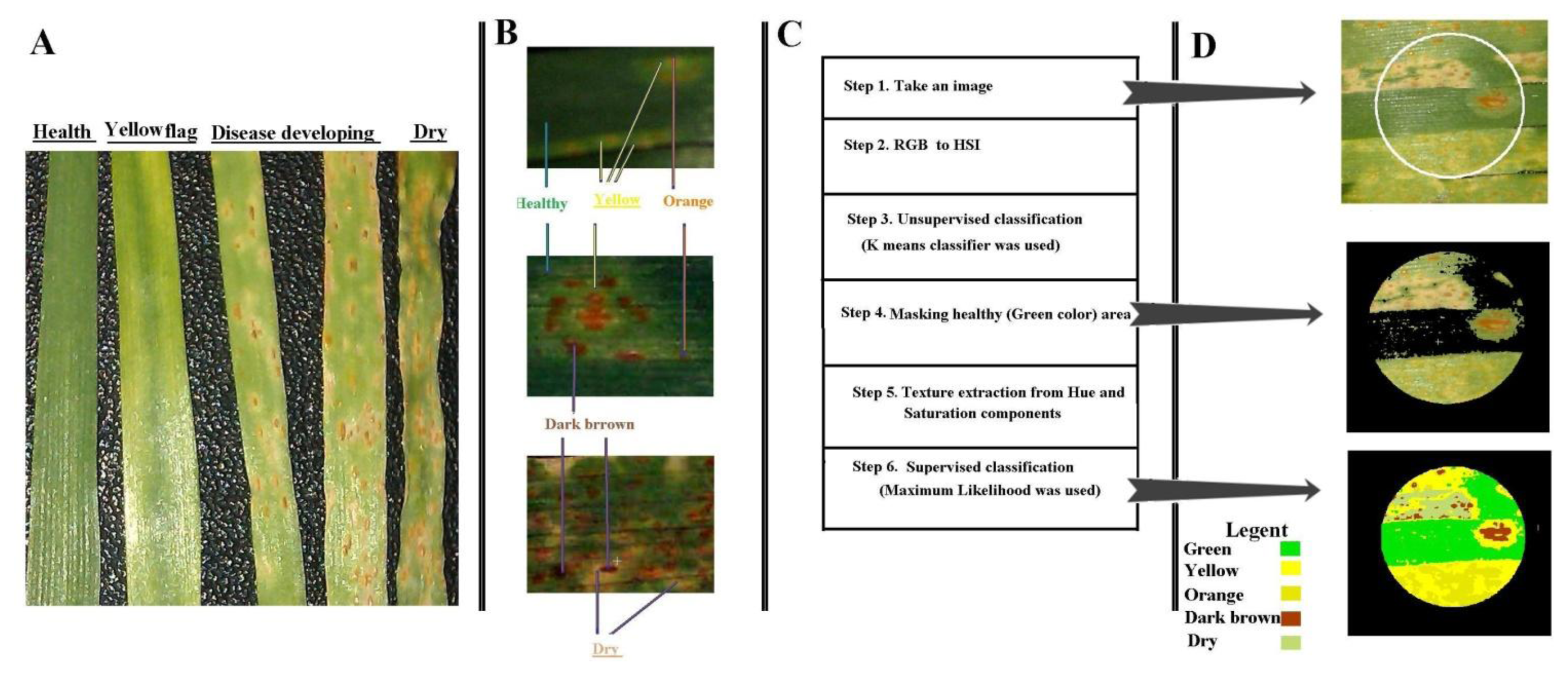
2.3.2. Extracting Disease Affected Fraction

To determine the ratio and symptoms of the leaf rust disease, a RGB digital camera with the following specifications was used: Camera model: Canon DIGITAL IXUS 85 IS; F-109 number: f/3.2; Shutter speed: 1/60. For all samples, the imaging height was 30 cm. Various symptoms of the leaf rust disease including yellow, orange, dark brown and the dry were extracted from the digital photos [14]. Different symptoms of the wheat rust have been illustrated in Figure 1A,B. After spectrometry, photography was performed outdoors. Therefore, in order to remove the effect of the light intensity, HIS system was used instead of the RGB system [20]. This algorithm is based on the transformation from the RGB to HIS space aiming to remove the effect of outdoor light intensity variations. Meanwhile, in this research, texture recognition algorithms were used to determine the boundaries of infected areas. Steps of classifying the disease symptoms by the images of the RGB digital camera are shown in Figure 1C. The amounts of different symptoms of the disease were determined by calculating the ratio of the areas of the infected spots to the total leaf area for each infected leaf. It must be taken into account that these measurements were conducted in the same area on which the spectrometry had been performed. The exact location of the spectral reflectance region on the leaf was marked with the contact probe so that the ratio and symptom of the disease could be extracted by the RGB digital camera. This area is displayed by a white circle in Figure 1D. Inside the marked area, a green mask was applied using a threshold value. The aim was to classify infected areas of the leaf with more precision. In addition, training samples were collected from the disease symptoms. Then, the maximum likelihood classification was applied on the H and S components in order to extract disease symptoms as shown in Figure 1C. The disease symptom fractions were used along with the spectra of the infected leaf as ground truth to evaluate the SVIs.

2.4. Spectral Vegetation Indices

The SVIs employed in this research include the common narrow-band ones such as the sensitivity to pigments, the indices independent of pigments, Chlorophyll absorption ratio index, the variables extracted from derivation of spectrum (maximum values of the first derivation of blue, red and yellow edges, sum of first derivation of blue, yellow, and red edge) and other variables related to SVIs such as the Greenness Index (GI), Normalized Difference Vegetation Index (NDVI), Narrow-band normalized difference vegetation index (NBNDVI), Nitrogen Reflectance Index (NRI), Photochemical Reflectance Index (PRI), The transformed chlorophyll Absorption and Reflectance Index (TCARI), Modified Simple Ratio (MSR), Plant Senescence Reflectance Index (PSRI), PhRI (Physiological Reflectance Index), Triangular Vegetation Index (TVI), Red-Edge Vegetation Stress Index (RVSI) and Anthocyanin Reflectance Index (ARI). The description of the total 22 indices can be seen in

Table 1. Description of vegetation indices.

Variable	Description
Db (Maximum value of 1st derivative within blue edge)	Blue edge covers 490–530 nm. Db is a maximum value of 1st order derivatives within the blue edge of 35 bands [21]
SDb (Sum of 1st derivative values within blue edge)	Defined by sum of 1st order derivative values of 35 bands within the blue edge [21]
Dy (Maximum value of 1st derivative within yellow edge)	Yellow edge covers 550–582 nm. Dy is a maximum value of 1st order derivatives within the yellow edge of 28 bands [21]
SDy (Sum of 1st derivative values within yellow edge)	Defined by sum of 1st order derivative values of 28 bands within the yellow edge [21]
Dr (Maximum value of 1st derivative within red edge)	Red edge covers 670–737 nm. Dr is a maximum value of 1st order derivatives within the red edge of 61 bands [21]
SDr (Sum of 1st derivative values within red edge)	Defined by sum of 1st order derivative values of 61 bands within the red edge [21]
GI (Greenness Index)	R554/R677 [22]
MSR (Modified Simple Ratio)	(R800/R670 − 1)/(R800/R670 + 1)1/2 [23,24]
NDVI (Normalized Difference Vegetation Index)	(RNIR − RR)/(RNIR + RR), where RNIR indicates 775–825 nm, RR indicates 650–700 nm, that include most key pigments [25]
NBNDVI (Narrow-band normalized difference vegetation index)	(R850 − R680)/(R850 + R680) [26]
NRI (Nitrogen Reflectance Index)	(R570 − R670)/(R570 + R670) [27]
PRI (Photochemical Reflectance Index)	(R570 − R531)/(R570 + R531) [28]
TCARI (the transformed chlorophyll Absorption and Reflectance Index)	3 × ((R700 − R670) − 0.2 × (R700 − R550) × (R700/R670)) [29]
SIPI (Structural Independent Pigment Index)	R800 − R445/R800 − R680 [30]
PSRI (Plant Senescence Reflectance Index)	(R680 − R500)/R750 [31]
PhRI (Physiological Reflectance Index)	(R550 − R531)/(R550 + R531) [28]
NPCI (Normalized Pigment Chlorophyll ratio Index)	(R680 − R430)/(R680 + R430) [32]
ARI (Anthocyanin Reflectance Index)	ARI = (R550)−1 − (R700)−1) [33]
TVI (Triangular Vegetation Index)	0.5(120(R750 − R550) − 200(R670 − R550)) [34]
CARI (Chlorophyll Absorption Ratio Index)	(|(a670 + R670 + b)|/(a2 + 1)1/2) × (R700/R670) [35] a = (R700 − R550)/150, b = R550 − (a × 550)
RVSI (Red-Edge Vegetation Stress Index)	((R712 + R752)/2) − R732 [36]
MCARI (Modified Chlorophyll Absorption in Reflectance Index)	(R701 − R671) − 0.2(R701 − R549)]/(R701/R671) [37]

[21–37]. Selected indices have been used to evaluate disease in various studies [8].

2.5. Investigation of SVIs

Assuming that different symptoms of a disease have various spectra [38], in a particular disease severity, distinct spectra of the disease symptoms with different fractions cause variations in the spectra recorded by the sensor. The sum of the first derivatives in the 450–1000 nm range was used as an indicator of a spectrum [19]. Variations of the first derivatives were computed at the specific disease severity level by Equation (1). Finally, the variations of spectra as a function of the disease severity were drawn. Results of the first derivative variations indicate at which disease severity level the sensitivity to disease symptoms is low.

Variations of the first derivative were calculated for specific disease severity levels by Equation (1).

$$\text{Variance}(\text{x})=\frac{1}{N}{\sum }_{i=1}^N{(x_i-m_i)}^2$$

(1)

For a single variate x, with a known mean value m, N is the number of data.

The first derivatives were used to examine the total wavelength range from 450 to 1000 nm, whereas SVIs are based on few wavelengths. It was expected, if there are variations in the first derivatives, this will certainly be reflected the index values.

In addition, the effect of the disease progress on each SVI was evaluated. SVIs have been developed to estimate different plant parameters using few wavelengths. The effect of the disease progress on SVIs was evaluated to understand the reaction of each SVI to disease severity. The within-class variance was measured by Equation (1) as a criterion to consider SVIs at different disease severity levels. It must be pointed out that the higher the value of the measure for the within-class variance the more difficult the detection of disease severity levels.

Disease progress from 0% to 100% of the leaf area was divided into 10 equal ranges. Each of the 10 regions of disease progress was assumed as one class. These regions were used to compute within-class and first derivative variance.

3. Results and Discussions

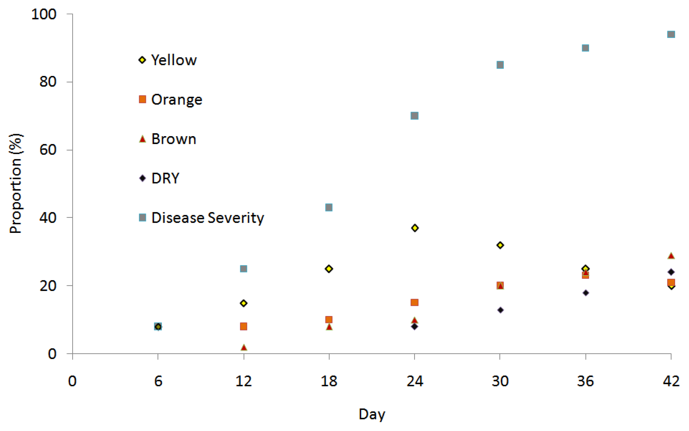
3.1. Disease Development in Leaves Inoculated with Rust

For each infected leaf, the proportions of different disease symptoms including yellow, orange, brown, dry, and the disease severity (the sum of the proportions of different disease symptoms) for 7, 14, 21, 28, 35, and 42 days after inoculation were extracted with a digital camera. On each day, about 50 leaves were evaluated randomly and the average of the proportions of different disease symptoms and disease severity were estimated.

Figure 2 shows the proportions of different disease symptoms and disease severity for a seven-day interval until the 42nd day after inoculation. On the 7th day after inoculation, the proportion of the yellow area is low, but it reaches the maximum value on day 21 (37%). However, the proportion of the yellow area decreases a little after 21 days. The orange and dark brown areas appear on the 14th day after inoculation and show an increasing trend. They reach their maximum values on day 42. The proportions of the orange and dark brown areas on day 42 are 23% and 24% of the leaf area, respectively. The dry area appears 28 days after inoculation and reaches its maximum (18%) on the 42nd day.

As shown in the Figure 2, disease severity which is the sum of the proportions of different disease symptoms increases with time after inoculation and peaks on day 42.

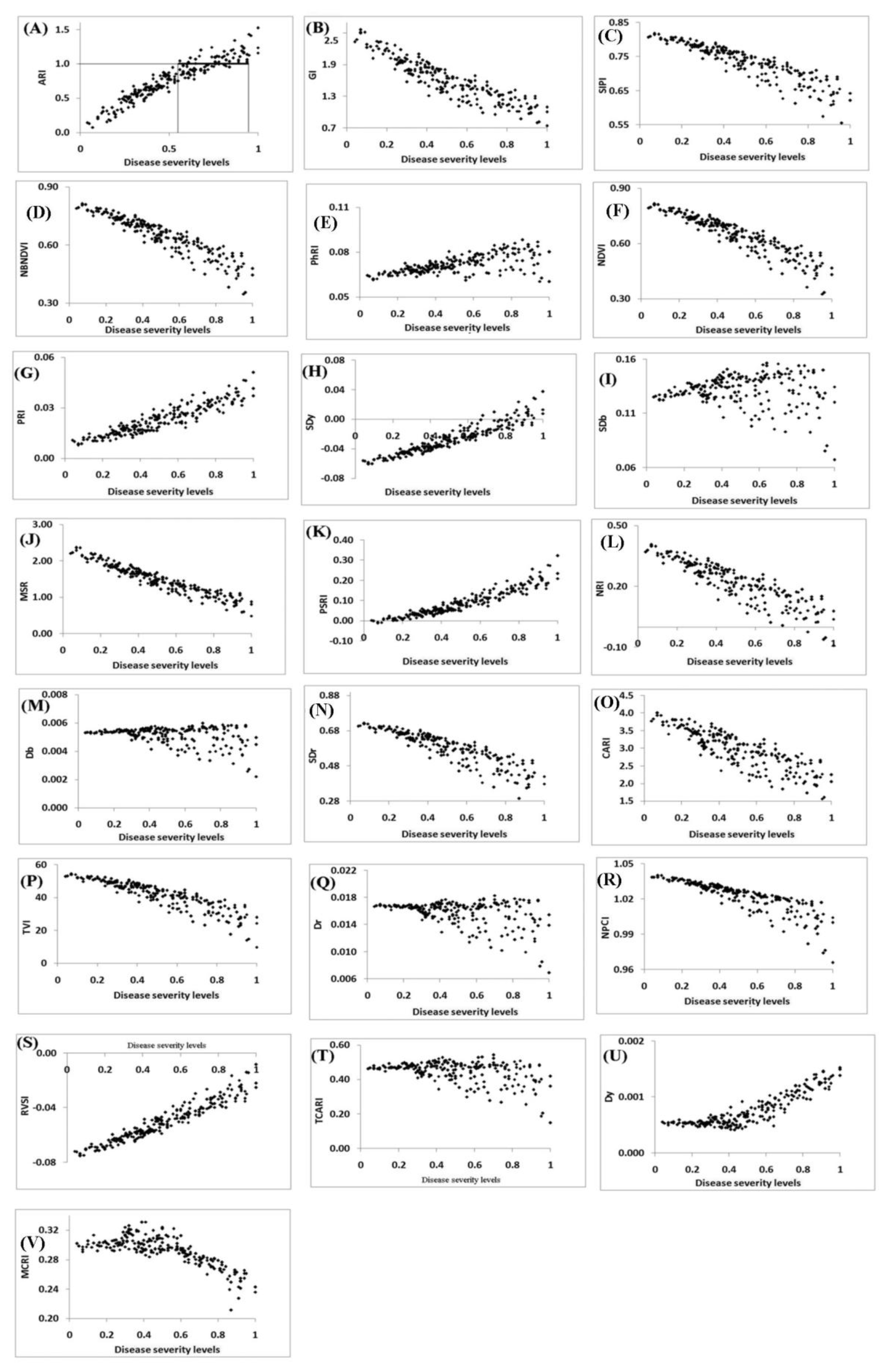
3.2. SVI Relationships with Disease Severity

Figure 3 demonstrates how the SVIs change as disease severity increases. The x and y vectors represent the disease severity levels (ratio of the leaf affected by the disease) and the numerical index values, respectively. According to Figure 3, as the disease severity increases, the scattering of the numerical values for all of the indices increases as well. However, SD_b, D_r, D_b and TCARI show more scattering (Figure 3I, M, Q, and T, respectively), while indices such as D_y and MCARI show erratic scattering (Figure 3U and V, respectively).

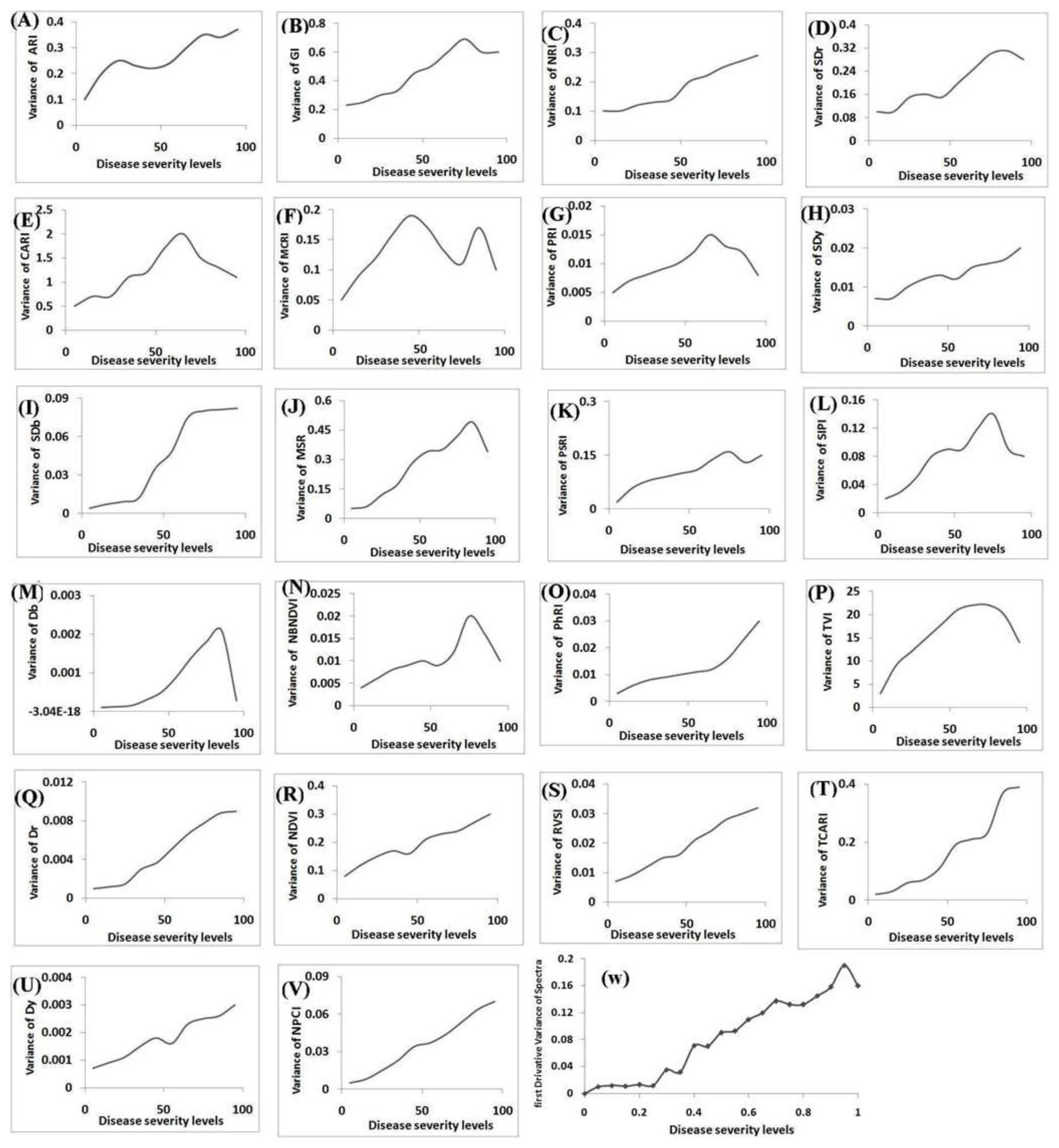
3.3. Evaluation of SVIs Variation

It was expected that as the disease progresses, the various disease symptoms will become more prominent. The within-class variance was calculated using Equation (1). The within-class variance was calculated for each disease level. Figure 4 demonstrates the changes of within-class variance as a function of disease severity levels for different indices.

Based on Figure 4, it can be concluded that for a great many of the SVIs, the within-class variance increases with the disease severity. However, the local decrease can be detected at some disease severity levels. Indices, such as D_y and MCARI, show different trends of scattering (Figure 4F,U, respectively).

The sum of the first derivatives in the 450–1000 nm range was used as the indicator of a spectrum. According to Figure 4W, as the disease severity increases, variations of the spectra also do. In addition, an increase in the spectra variation causes scattering in computed SVIs.

As shown in Figure 4, the variance of most of the SVIs increases as the disease develops. It is expected as variance declines, the SVIs classification accuracy increases in disease detection.

3.4. SVIs Capability to Detect Disease

The results show that as the disease develops so do the spectral variation and SVIs scattering. The Classification accuracy and error were used in order to choose the suitable SVI for disease estimation. The classification accuracy of SVIs to discriminate the healthy and infected areas has been shown in

Table 2. Comparison of the classification accuracy of Spectral Vegetation Indices (SVIs) to discriminate rust and healthy.

Index	Classification Accuracy	Recall		Index	Classification Accuracy	Recall
		Rust	Healthy			Rust	Healthy
Db	12%	11%	14%	TCARI	15%	17%	14%
SDb	14%	15%	12%	SIPI	73%	70%	75%
Dy	29%	31%	27%	PSRI	69%	71%	67%
SDy	9%	11%	8%	PhRI	71%	72%	69%
Dr	16%	15%	17%	NPCI	68%	67%	69%
SDr	13%	10%	15%	ARI	75%	73%	78%
GI	77%	81%	75%	TVI	69%	71%	68%
MSR	68%	65%	71%	NRI	67%	71%	65%
NDVI	81%	79%	83%	PRI	12%	11%	14%
NBNDVI	83%	84%	82%	MCRI	38%	36%	39%

. SDy and NBNDVI show the lowest and highest classification accuracy, respectively. After NBNDVI, SVIs such as NDVI, GI, ARI, SIPI, and PHRI show classification accuracy more than 70%.

Classification error of SVIs at 10 disease severity levels was measured. As the SVIs showed different levels of sensitivity to disease progress, a variety of classification errors was expected. According to the classification error results, SVIs were categorized in three groups. The first group showed low classification errors. This group includes NBNDVI, NDVI, GI, ARI, and PRI, as

Table 3. Classification error of SVIs at different disease severity levels. NDVI, PRI, NBNDVI and GI from the first group show low Classification error. TCARI, SD_b, D_b, D_r of the second group of SVIs show high classification error. MCRI and SD_y of the third group of SVIs show erratic classification error.

Disease Severity	Classification Error %
	NBNDVI		NDVI		PRI		GI		TCARI
	Healthy	Rust	Healthy	Rust	Healthy	Rust	Healthy	Rust	Healthy	Rust
1%–5%	25	34	29	38	44	43	31	34	32	36
5%–10%	12	14	13	14	11	19	16	18	23	17
10%–20%	11	12	14	10	13	18	14	12	19	19
20%–30%	15	10	17	14	17	15	13	13	21	27
30%–40%	14	13	26	18	11	22	18	14	19	19
40%–50%	25	21	26	28	21	28	22	24	27	18
50%–60%	28	29	19	37	29	32	23	23	26	37
60%–70%	31	37	44	36	34	47	33	33	41	43
70%–80%	38	55	47	54	44	61	36	51	52	54
>80%	53	44	61	52	49	58	46	40	61	39
Disease Severity	Classification Error %
	SDb		Db		Dr		Dy		MCRI
	Healthy	Rust	Healthy	Rust	Healthy	Rust	Healthy	Rust	Healthy	Rust
1%–5%	81	82	79	82	91	90	88	85	91	92
5%–10%	90	92	75	83	79	93	75	85	80	88
10%–20%	91	77	85	93	90	83	85	83	79	83
20%–30%	94	88	83	78	79	93	95	88	84	77
30%–40%	86	88	88	88	86	78	94	79	66	68
40%–50%	84	79	79	84	84	86	43	44	39	34
50%–60%	84	37	86	84	84	91	32	27	27	24
60%–70%	79	88	82	79	79	89	37	31	31	18
70%–80%	80	69	80	81	79	77	19	20	19	20
>80%	77	71	82	79	77	72	23	24	21	19

shows. These indices show high classification errors in the 1%–5% disease severity range. For example, NBNDVI shows errors of 45% and 55% for rust and other classes, respectively. However, for levels between 5% and 10%, the classification errors of NBNDVI, NDVI, PRI, and GI are less than 20%.

For disease severity levels of more than 40%, the error increases again. Finally, the error reaches around 50% for disease severity levels of more than 70%. The second group of SVIs includes SD_b, D_r, D_b, TCARI, and phRI that show high classification errors at all disease severity levels. The classification error slightly declines at the disease severity levels more than 70%. The error of these indices has been shown in Table 3.

The third group of SVIs includes MCRI and SD_y that show an erratic relationship with disease severity levels. As Table 3 shows, the classification error of MCRI and SD_y are around 70% for disease severity levels ranging from 0% to 50%. At severity levels more than 40%, the classification error decreases suddenly.

Using the first derivative showed spectrum variations at disease severity levels. Spectrum variations cause scattering of SVIs as the disease develops. Scattering of an SVI clearly has increased classification errors. Although the scattering of SVIs were low at disease severity levels between 0% and 5%, the classification error was high. This is due to the similarity of reflectance of healthy and infected leaves at first symptoms of disease.

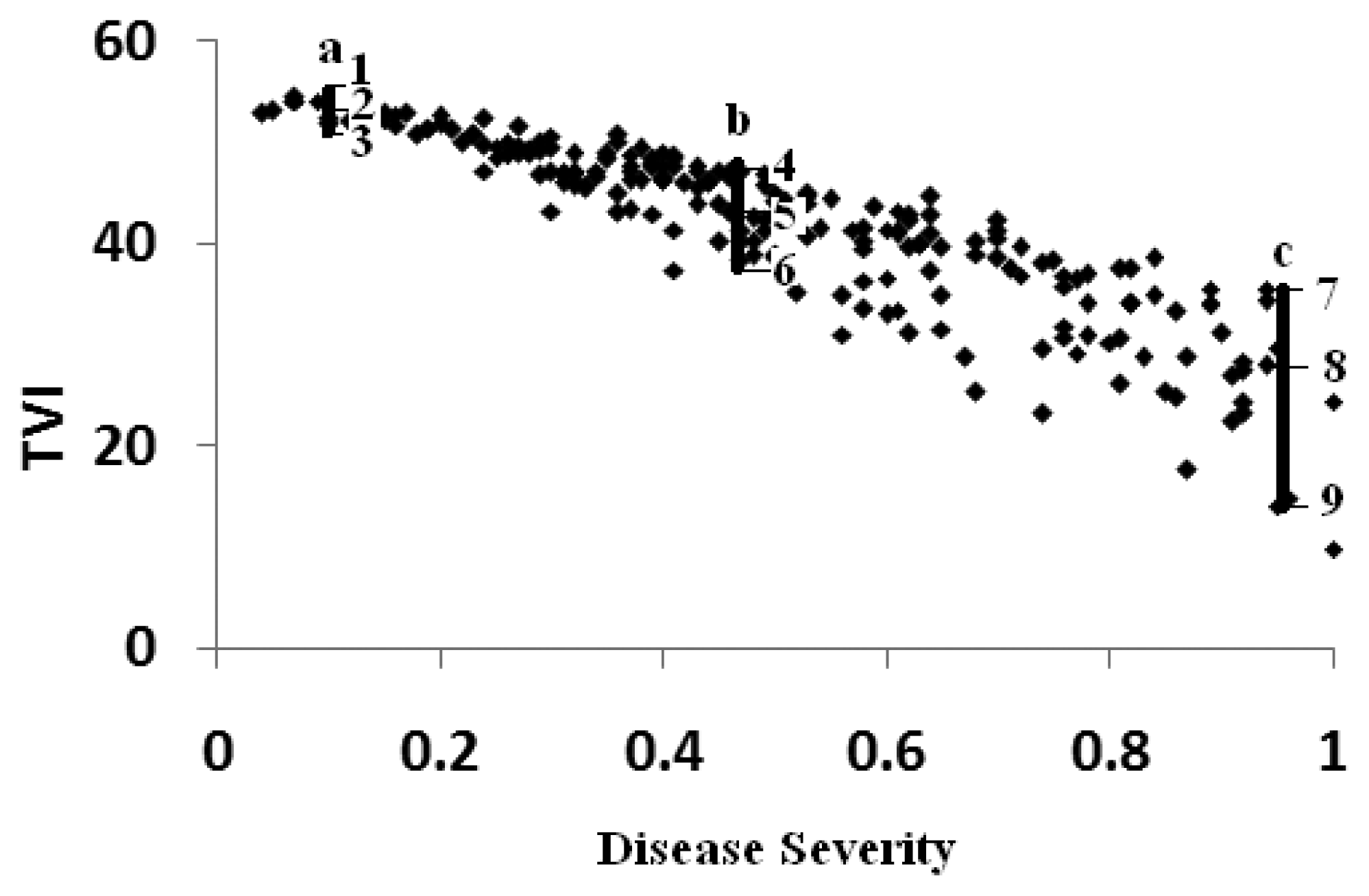
3.5. Scattering of SVI with Disease Severity

The effect of the disease symptoms on SVIs was investigated considering the scattering pattern of SVIs as the disease develops. Figure 5 illustrates the relationship between one of the SVIs (TVI), which shows high scattering, and the disease severity. Every point on the scatter plot shows the TVI value of a measured spectrum with known disease symptom fractions. 3 lines are shown on Figure 5 on each of which three points were chosen. Points 1, 2, and 3 on line a, points 4, 5, and 6 on line b, and points 7, 8, and 9 on line c. The disease severity levels for lines a, b and c are 0.1, 0.5 and 0.95, respectively. The points over each line have the same disease severity levels but different index values. These different index values at the same disease severity level cause scattering. Scattering of the data reduces the TVI accuracy in disease detection. The scattering is caused by changes in disease symptom proportions from a point to another one for the same disease severity level. The disease symptom fractions are illustrated for every point in

Table 4. The fractions of disease symptoms at three different disease severity levels for Triangular Vegetation Index (TVI).

Line Number	Point Number	Green %	Yellow %	Orange %	Dark Brown %	Dead %
A	1	90	7	3	0	0
A	2	90	5	5	0	0
A	3	91	8	3	0	0
B	4	50	7	12	11	20
B	5	51	19	18	11	2
B	6	50	17	13	15	5
C	7	6	12	28	21	33
C	8	5	11	9	7	47
C	9	5	10	11	15	59

.

As indicated by lines a, b, and c in Table 4, a point on each line contains different amounts of green, yellow, orange, brown, and dry values compared with other points on the same line. Based on Figure 4, it can be stated that although the disease severity of lines a, b, and c has remained fixed, the index value has changed. As shown in Table 4, index value scattering can be explained by different disease symptom fractions for the same disease severity. For example, points 7 and 9 at the same disease severity level (0.95) have different disease symptom fractions (Table 4); especially, the fraction of the dry area at point 9 is more than point 7. The fractions of the dry area are 59% and 33% for points 9 and 7, respectively. Figure 4 indicates that although the disease severity has fixed values over each line, the index value varies considerably due to different disease symptom fractions of the points.

As Figure 3 shows, the scattering of SVIs are different. The reason for the scattering at a specific disease severity is the presence of different combinations of disease symptoms. Collected spectra in this research contain mixed information over a certain area of the leaf. The proportions of the healthy to the diseased area change. In addition, in the diseased area, the proportion of different disease symptoms changes during pathogenesis. As studies have shown in the past [38], each symptom has a distinct spectrum. Therefore, the collected spectra are mixed and their reflectance values depend on the fractions of the disease symptoms.

Figure 2 shows that the multiplicity of disease symptoms increases as the disease severity does. SVIs show different sensitivities to an increase in disease severity (Figures 3 and 4). The amount of scattering is higher for some SVIs such as the second and third groups. The high scattering for such SVIs causes the classification error to increase. On the other hand, the first group of SVIs is less sensitive to disease symptoms and displays lower amounts of scattering (NBNDVI, NDVI, GI, ARI, and PRI). According to Table 3 and Figure 3, as the extent of scattering decreases, the classification accuracy of disease severity levels increases.

4. Conclusions

The results of this research showed that the disease symptoms have high impact on the infected plant spectra. The first derivative of the spectrum from 450 to 1000 nm can be used as its signature. A direct relationship was found to exist between the first derivative variation and the disease severity. It means that as the disease severity increases, so do the collected spectrum variations at a specific disease severity. It is expected that for a specific disease, as the number of disease symptoms increases, the spectra will become more complex at a specific disease severity level. All of the SVI values were sensitive to disease severity so that the classification accuracy decreased as the disease severity increased. For the different SVIs, the amounts of scattering and classification accuracy are not the same and depend on the wavelength(s) used. Difficulty remained in the early detection of the disease when the disease severity was less than 5%, due to minor changes of reflectance. However, for levels between 5% and 10%, the classification errors of the proposed indices (NBNDVI, NDVI, PRI, and GI) were low. Suitable SVIs for the detection of leaf rust also showed less classification accuracy in disease severity cases of more than 50%, because of the multiplicity of disease symptoms. Nevertheless, SVIs are valuable due to the reduction of data dimensionality and data processing. It is necessary to consider more carefully the capability of SVIs for the detection of plant diseases, especially for the diseases with different symptoms. It must be noted that the proposed SVIs need to be tested on various sensors and different varieties of wheat in order to be used in precision farming.

The results of this research demonstrated that the spectral mixture of disease symptoms must be taken into account in leaf disease studies. As a concluding remark, it must be mentioned that the spectral mixture analysis of disease symptoms reduces SVIs accuracy; however, it makes possible the estimation of disease symptoms.

References

1. Roelofsen, H.D.; van Bodegom, P.M.; Kooistra, L.; Witte, J.-P.M. Trait estimation in herbaceous plant assemblages from in situ canopy spectra. Remote Sens 2013, 5, 6323–6345. [Google Scholar]
2. Delalieux, S.; Auwerkerken, A.; Verstraeten, V.W.; Somers, B.; Valcke, R.; Lhermitte, S.; Keulemanss, J.; Coppin, P. Hyperspectral reflectance and fluorescence imaging to detect scab induced stress in Apple leaves. Remote Sens 2009, 1, 858–874. [Google Scholar]
3. Steiner, U.; Bürling, K.; Oerke, E.-C. Sensor use in plant protection. Gesunde Pflanz 2008, 60, 131–141. [Google Scholar]
4. Zhang, J.; Pu, R.; Huang, W.; Yuan, L.; Luo, J.; Wang, J. Using in-situ hyperspectral data for detecting and discriminating yellow rust disease from nutrient stresses. Field Crops Res 2012, 134, 165–174. [Google Scholar]
5. Hillnhütter, C.; Mahlein, A.-K.; Sikora, R.A.; Oerke, E.-C. Remote sensing to detect plant stress induced by heterodera schachtii and rhizoctonia solani in sugar beet fields. Field Crops Res 2011, 122, 70–77. [Google Scholar]
6. Moshou, D.; Bravo, C.; West, J.; Wahlen, S.; McCartney, A.; Ramon, H. Automatic detection of “yellow rust” in wheat using reflectance measurements and neuralnetworks. Comput. Electron. Agric 2004, 44, 173–188. [Google Scholar]
7. Mahlein, A.-K.; Rumpf, T.; Welke, P.; Dehne, H.-W.; Plümer, L.; Steiner, U.; Oerke, E.-C. Development of spectral indices for detecting and identifying plant diseases. Remote Sens. Environ 2013, 128, 21–30. [Google Scholar]
8. Zhang, J.-C.; Pu, R.-L.; Wang, J.-H.; Huang, W.-J.; Yuan, L.; Luo, J.-H. Detecting powdery mildew of winter wheat using leaf level hyperspectral measurements. Comput. Electron. Agric 2012, 85, 13–23. [Google Scholar]
9. Gitelson, A.A.; Kaufman, Y.J.; Stark, R.; Rundquist, D. Novel algorithms for remote estimation of vegetation fraction. Remote Sens. Environ 2002, 80, 76–87. [Google Scholar]
10. Peñuelas, J.; Baret, F.; Filella, I. Semiempirical indices to assess carotenoids/chlorophyll a ratio from leaf spectral reflectance. Photosynthetica 1995, 31, 221–230. [Google Scholar]
11. Rumpf, T.; Mahlein, A.-K.; Steiner, U.; Oerke, E.-C.; Dehne, H.-W.; Plümer, L. Early detection and classification of plant diseases with support vector machines based on hyperspectral reflectance. Comput. Electron. Agric 2010, 74, 91–99. [Google Scholar]
12. Mahlein, A.-K.; Steiner, U.; Dehne, H.-W.; Oerke, E.-C. Spectral signatures of sugar beet leaves for the detection and differentiation of diseases. Precis. Agric 2010, 11, 413–431. [Google Scholar]
13. Bolton, M.; Kolmer, J.; Garvin, D. Wheat leaf rust caused by Puccinia triticina. Mol. Plant Patol 2008, 9, 563–575. [Google Scholar]
14. Robert, C.; Bancal, M.-O.; Ney, B.; Lannou, C. Wheat leaf photosynthesis loss due to leaf rust, with respect to lesion development and leaf nitrogen status. New Phytol 2005, 165, 227–241. [Google Scholar]
15. Hansen, J.G. Use of multispectral radiometry in wheat yellow rust experiments. OEPP/EPPO Bull 1991, 21, 651–658. [Google Scholar]
16. Huang, W.; Lamb, D.W.; Niu, Z.; Zhang, Y.; Liu, L.; Wang, J. Identification of yellow rust in wheat using in-situ spectral reflectance measurements and airborne hyperspectral imaging. Precis. Agric 2007, 8, 187–119. [Google Scholar]
17. West, J.S.; Bravo, C.; Oberti, R.; Lemaire, D.; Moshou, D.; McCartney, H.A. The potential of optical canopy measurement for targeted control of field crop diseases. Annu. Rev. Phytopathol 2003, 4, 593–614. [Google Scholar]
18. Devadas, R.; Lamb, D.W.; Simpfendorfer, S.; Backhouse, D. Evaluating ten spectral vegetation indices for identifying rust infection in individual wheat leaves. Precis. Agric 2009, 10, 459–470. [Google Scholar]
19. Franke, J.; Menz, G. Multi-temporal wheat disease detection by multi-spectral remote sensing. Precis. Agric 2007, 8, 161–172. [Google Scholar]
20. Al-Hiary, H.; Bani-Ahmad, S.; Reyalat, M.; Braik, M.; ALRahamneh, Z. Fast and accurate detection and classification of plant diseases. Int. J. Comput. Appl 2011, 17, 31–38. [Google Scholar]
21. Gong, P.; Pu, R.; Heald, R.C. Analysis of in situ hyperspectral data for nutrient estimation of giant sequoia. Int. J. Remote Sens 2002, 23, 1827–1850. [Google Scholar]
22. Zarco-Tejada, P.J.; Berjón, A.; López-Lozano, R.; Miller, J.R.; Martín, P.; Cachorro, V.; González, M.R.; Frutos, A. Assessing vineyard condition with hyperspectral indices: Leaf and canopy reflectance simulation in a row-structured discontinuous canopy. Remote Sens. Environ 2005, 99, 271–287. [Google Scholar]
23. Chen, J.M. Evaluation of vegetation indices and a modified simple ratio for boreal applications. Can. J. Remote Sen 2000, 22, 229–242. [Google Scholar]
24. Haboudane, D.; Miller, J.R.; Pattery, E.; Zarco-Tejad, P.J.; Strachan, I.B. Hyperspectral vegetation indices and novel algorithms for predicting green LAI of crop canopies: Modeling and validation in the context of precision agriculture. Remote Sens. Environ 2004, 90, 337–352. [Google Scholar]
25. Rouse, J.W.; Haas, R.H.; Schell, J.A.; Deering, D.W. Monitoring Vegetation Systems in the Great Plains with ERTS. Proceedings of the 1973 Earth Resources Technology Satellite-1 Symposium, Washington, DC, USA, 10–14 December 1973.
26. Thenkabail, P.S.; Smith, R.B.; de Pauw, E. Hyperspectral vegetation indices and their relationships with agricultural crop characteristics. Remote Sens. Environ 2000, 71, 158–182. [Google Scholar]
27. Filella, I.; Serrano, L.; Serra, J.; Penuelas, J. Evaluating wheat nitrogen status with canopy reflectance indices and discriminant analysis. Crop Sci 1995, 35, 1400–1405. [Google Scholar]
28. Gamon, J.A.; Penuelas, J.; Field, C.B. A narrow-waveband spectral index that tracks diurnal changes in photosynthetic efficiency. Remote Sens. Environ 1992, 41, 35–44. [Google Scholar]
29. Haboudane, D.; John, R.; Millera, J.R.; Tremblay, N.; Zarco-Tejada, P.J.; Dextraze, L. Integrated narrow-band vegetation indices for prediction of crop chlorophyll content for application to precision agriculture. Remote Sens. Environ 2002, 81, 416–426. [Google Scholar]
30. Penuelas, J.; Gamon, J.A.; Fredeen, A.L.; Merino, J.; Field, C.B. Reflectance indices associated with physiological changes in nitrogen- and water-limited sunflower leaves. Remote Sens. Environ 1995, 48, 135–146. [Google Scholar]
31. Merzlyak, M.N.; Gitelson, A.A.; Chivkunova, O.B.; Rakitin, V.Y. Non-destructive optical detection of pigment changes during leaf senescence and fruit ripening. Physiol. Plant 1999, 106, 135–141. [Google Scholar]
32. Penuelas, J.; Pinol, J.; Ogaya, R.; Filella, I. Estimation of plant water concentration by the reflectance water index WI (R900/R970). Int. J. Remote Sens 1997, 18, 2869–2875. [Google Scholar]
33. Gitelson, A.A.; Merzlyak, M.N.; Chivkunova, O.B. Optical properties and nondestructive estimation of anthocyanin content in plant leaves. Photochem. Photobiol 2001, 74, 38–45. [Google Scholar]
34. Broge, N.H.; Leblanc, E. Comparing prediction power and stability of broadband and hyperspectral vegetation indices for estimation of green leaf area index and canopy chlorophyll density. Remote Sens. Environ 2000, 76, 156–172. [Google Scholar]
35. Kim, M.S.; Daughtry, C.S.T.; Chappelle, E.W.; McMurtrey, J.E. The Use of High Spectral Resolution Bands for Estimating Absorbed Photosynthetically Active Radiation (APAR). Proceedings of the 1994 International Symposium on Physical Measurements and Signatures in Remote Sensing, Val d’Isère, France, 1 January 1994.
36. Merton, R.; Huntington, J. Early Simulation of the ARIES-1 Satellite Sensor for Multi-Temporal Vegetation Research Derived from AVIRIS. In Summaries of the Eight JPL Airborne Earth; Jet Propulsion Laboratory, National Aeronautics and Space Administration: Pasandena, CA, USA, 1999; pp. 299–307. [Google Scholar]
37. Daughtry, C.S.; Walthall, C.L.; Kim, M.S.; de Colstoun, E.B.; McMurtrey, J.E. Estimating corn leaf chlorophyll concentration from leaf and canopy reflectance. Remote Sens. Environ 2000, 74, 229–239. [Google Scholar]
38. Mahlein, A.-K.; Steiner, U.; Hillnhütter, C.; Dehne, H.-W.; Oerke, E.-C. Hyperspectral imaging for small-scale analysis of symptoms caused by different sugar beet diseases. Plant Methods 2012, 8. [Google Scholar] [CrossRef]
Figure 1. (A) Disease progress of wheat leaf rust; (B) different symptoms of wheat leaf rust; (C) classification steps of disease symptoms of wheat leaf rust by RGB digital camera; (D) classification of different symptoms and masking green area of wheat leaf rust, the leaf area (Four leaves were placed next to each other) marked by the contact probe is shown by the white circle).
Remotesensing 06 05107f1
Figure 2. Proportion of disease severity and different disease symptoms in wheat flag leaf infected by Puccinia triticina from day 7 to 42 after inoculation.
Remotesensing 06 05107f2
Figure 3. The relationship between the SVIs and the disease severity. (AF) SVIs with low scattering; (GT) show SVIs with high scattering; (U,V) show SVIs with erratic scattering.
Remotesensing 06 05107f3
Figure 4. (AV) The relationship between disease severity levels and the variance of SVIs. (W) shows the sum of the first derivatives relationship and disease severity.
Remotesensing 06 05107f4
Figure 5. Relationship between the TVI and disease severity to evaluate scattering. Disease severity is constant over each line (lines a, b, and c).
Remotesensing 06 05107f5