Daytime Low Stratiform Cloud Detection on AVHRR Imagery

Abstract

The near-real time retrieval of low stratiform cloud (LSC) coverage is of vital interest for such disciplines as meteorology, transport safety, economy and air quality. Within this scope, a novel methodology is proposed which provides the LSC occurrence probability estimates for a satellite scene. The algorithm is suited for the 1 × 1 km Advanced Very High Resolution Radiometer (AVHRR) data and was trained and validated against collocated SYNOP observations. Utilisation of these two combined data sources requires a formulation of constraints in order to discriminate cases where the LSC is overlaid by higher clouds. The LSC classification process is based on six features which are first converted to the integer form by step functions and combined by means of bitwise operations. Consequently, a set of values reflecting a unique combination of those features is derived which is further employed to extract the LSC occurrence probability estimates from the precomputed look-up vectors (LUV). Although the validation analyses confirmed good performance of the algorithm, some inevitable misclassification with other optically thick clouds were reported. Moreover, the comparison against Polar Platform System (PPS) cloud-type product revealed superior classification accuracy. From the temporal perspective, the acquired results reported a presence of diurnal and annual LSC probability cycles over Europe.

1. Introduction

Low stratiform clouds (LSC) are of great importance for a wide range of disciplines including meteorology [1], transportation [2,3], economy [4] and air quality [5,6]. In terms of financial losses, the impact of reduced horizontal visibility associated with the LSC is comparable to tornado damages [7], thus there is a strong need for development of low-cloud monitoring systems. A network of ground synoptic stations provides detailed point visibility and cloud-base measurements at high temporal resolution, but only over highly populated areas. Furthermore, the measurements are performed in manual or automatic ways by various types of instruments, which complicates derivation of homogeneous data records. In this respect, spaceborne observations of the LSC cover benefit from their vast spatial coverage, high temporal sampling and consistent measuring technique. These features are of great importance for operational weather forecasting [1] and climatic research [8] and are only available by means of the remote sensing techniques [9]. There is substantial diversity in the definition of remotely sensed LSC products. Low stratus and fog covers might be combined due to their similar spectral signatures [10,11] or additional effort can be made to delineate only the conditions with reduced horizontal visibility [12]. In this study these categories are treated together as the LSC. The main intention for the development of the proposed method was to facilitate weather nowcasting systems by providing near-real time LSC coverage information supplemented by probability estimates.

The next section elaborates on the definition and properties of the LSC cover. Section 3 presents an overview on existing algorithms for the satellite LSC detection. Sections 4 and 5 describe the required datasets and the proposed methodology. In Section 6 the acquired classification results are discussed. Finally, overall conclusions about the proposed method for LSC detection on AVHRR imagery are drawn in Section 7.

2. Characteristics of Low Stratiform Clouds

The main focus of this study is on low-level clouds composed of stratus and fog layers. Therefore, in order to describe the LSC cover, two separate definitions are required. According to classification provided by the World Meteorological Organisation [13], the basic discrimination of clouds corresponds to their base heights: low (<2 km), middle (2–7 km) and high (5–13 km). Furthermore, they are divided into genus types, species, varieties and supplementary features which were combined in nine classes per altitude level, resulting in 27 categories in total (

Table 1. SYNOP cloud type codes from the C0000000000000013000 bufr table.

Code	Description
11	cirrus fibratus or cirrus uncinus
12	cirrus spissatus, in patches or entangled sheaves
13	cirrus spissatus cumulonimbogenitus
14	cirrus uncinus or fibratus,or both, progressively invading the sky
15–16	cirrus (often in bands) and cirrostratus, or cirrostratus alone with the continuous veil
17	cirrostratus covering the whole sky
18	cirrostratus not progressively invading the sky and not entirely covering it
19	cirrocumulus alone, or cirrocumulus predominant among others high clouds
21	altostratus translucidus
22	altostratus opacus or nimbostratus
23	altocumulus translucidus at a single level
24	patches (often lenticularis) of altocumulus translucidus
25	altocumulus translucidus in bands, or layers of altocumulus translucidus or opacus
26	altocumulus cumulogenitus (or cumulonimbogenitus)
27	altocumulus translucidus or opacus, or altocumulus opacus in a single layer
28	altocumulus castellanus or flocus
29	altocumulus of chaotic sky, generally at several levels
31	cumulus humilis or cumulus fractus other than of bad weather, or both
32	cumulus mediocris or congestus
33	cumulonimbus calvus, with or without cumulus, stratocumulus or stratus
34	stratocumulus cumulogenitus
35	stratocumulus other than stratocumulus cumulogenitus
36	stratus nebulosus or stratus fractus other than of bad weather, or both
37	stratus fractus or cumulus fractus of bad weather usually below altostratus or nimbostratus
38	cumulus and stratocumulus other than stratocumulus cumulogenitus
39	cumulonimbus capillatus (often with an anvil)

). This classification is utilised in the surface synoptic observations reports (SYNOP), which were employed in the scope of performed analyses as reference and validation data. However, it does not include a fog cover that, for the sake of synoptic reports, is not regarded as a cloud but as reduced visibility [14]. More specifically, fog is associated with the reduction of horizontal visibility below 1 km [7,15,16]. However, it may be treated as a stratiform cloud [17] that reaches the surface, or as precipitation [18], depending on a context of the analysis.

As far as the definition of LSC is concerned, this study follows the convention proposed by [19], who recognised LSC as an assembly of stratus and stratocumulus clouds together with the fog coverage. They also included the fractocumulus and fractostratus clouds, which are associated with non-stratiform or middle-altitude clouds in the SYNOP classification (codes 31, 37 in Table 1). Therefore, in this study, the LSC cover corresponds to codes: 34, 35, 36 and 38 in Table 1. Moreover, from the “present weather” SYNOP report, the following codes [20] associated with a fog occurrence were selected after [21]: 11, 12, 40–49 (

Table 2. SYNOP present weather codes from the C0000000000000013000 bufr table.

Code	Description
10	mist
11	patches of shallow fog or ice fog at station
12	more or less continuous shallow fog or ice fog at station
40	fog or ice fog at a distance at the time of observation but not at station
41	fog or ice fog in patches
42	fog or ice fog, sky visible, has become thinner during the preceding hour
43	fog or ice fog, sky invisible, has become thinner during the preceding hour
44	fog or ice fog, sky visible, no appreciable change during the preceding hour
45	fog or ice fog, sky invisible, no appreciable change during the preceding hour
46	fog or ice fog, sky visible, has become thicker during the preceding hour
47	fog or ice fog, sky invisible, has become thicker during the preceding hour
48	fog depositing rime sky visible
49	fog depositing rime sky invisible

).

2.1. Physical Properties of Stratiform Clouds

Detection of LSC by means of remote-sensing techniques requires broad knowledge of their physical properties that result in a particular spectral signature on satellite images. Characteristics of fog derived from the AVHRR data were explored in the study of [5]. Bendix determined that, on average, optical depth of fog equals 10.5 with a standard deviation (SD) of 9.1; droplet effective radius equals 7.14 with SD of 9.98; and liquid water path (LWP) equals 34.2 g/m² with SD of 21.1 g/m². The maximal geometrical thickness of the fog layer should not exceed 400 m [22]. The droplet number per air volume may vary from a few droplets to 100 per cm³ and may change significantly regardless of the total LWP [23]. On the other hand, stratus clouds in comparison to fog have a greater geometrical thickness of around 900 m, but a similar optical depth of 21.3–26.3, effective droplet size distribution of 5–12 μm and LWP 129.0–133.6 g/m² [24]. Therefore, a straightforward way to distinguish these two cloud types is to compute cloud top height (CTH) which for fog should not exceed 400 m. However, low-cloud top height does not directly indicate reduced visibility at the ground level in cases when low stratus or elevated fog are suspended above the surface. In such a situation, cloud geometrical thickness could be theoretically estimated on the basis of cloud physical properties [12]. Some solutions to this issue involve simple parameterisation of the geometrical thickness ΔZ as a function of optical depth. Other approaches [25] assume adiabatic increase of the cloud LWP with altitude up to its top which is related to the ΔZ through the temperature-dependent moist-adiabatic condensate coefficient. More advanced techniques [12] relate different penetration depths of the electromagnetic radiation within a cloud at certain spectral ranges (0.65, 1.64 and 2.1 μm) to the ΔZ by means of the iterative least square variance minimisation. Ultimately, the cloud/fog base height is computed by subtracting the geometrical thickness from its top height altitude. Nevertheless, for low clouds, the error of cloud top height retrieval is much greater than 400 m and, for instance, it equals 773 m on average for the Polar Platform System (PPS) CTH product [26]. Furthermore, cloud physical properties derivation adds another uncertainty to the geometrical thickness retrieval; therefore, this quantity can be only useful for climatological studies. Consequently, passive radiometers such as AVHHR do not provide sufficient information to assess if a cloud has physical contact with the surface. Thus, in this study, fog and low stratiform clouds together are considered to be the LSC.

2.2. Spectral Properties of Stratiform Clouds

Physical characteristics of LSC cover determine its interaction with the electromagnetic radiation. Concerning the IR spectrum, the LSC in liquid phase feature lower emissivity at 3.7 μm in comparison to the 10.8 μm wavelength range. Therefore, during the night for LSC, the 3.7–10.8 μm brightness temperature difference (BTD) is small or negative. Conversely, during the day, solar radiation contributes to the 3.7 μm signal, thereby making the difference positive. Consequently, it varies significantly with the sun zenith angle (SZA), which makes its parametrisation complex in the satellite LSC detection schemes. In this case, the reflective part of the 3.7 μm spectrum can be derived by subtracting a thermal component approximated by the 10.8 μm brightness temperature (BT) under the assumption of unit emissivity [27–29]. Furthermore, the retrieved reflectance should be normalised by the cosine of the SZA and corrected for the sun–earth distance variation. This makes the 3.7 μm reflectance almost independent of the illumination conditions [30]. Nevertheless, both reflective and thermal components of the 3.7 μm spectra depend on the cloud droplet size, underlying surface properties and sensor’s viewing zenith angle (VZA). This in turn implies that the LSC, which have generally smaller droplet sizes than higher clouds, are more reflective at this wavelength, and that the absolute 3.7–10.8 μm BTD is greater [30]. However, similar spectral characteristics are associated with low-emissivity deserts [11], thus these features have to be treated separately over such areas in the satellite cloud detection schemes [31]. Similar difficulties are related to the marine stratiform clouds which have larger droplets due to the smaller amount of cloud condensation nuclei (CCN) [32]. This results in low 3.7 μm reflectance and small 3.7–10.8 μm BTD, which is comparable to the clear-sky water background [30]. On the other hand, separation of clouds in different thermodynamic phases is less complicated as ice crystals are generally larger than water droplets, thus resulting in greater transmissivity in the shortwave infrared window, low 1.6 & 3.7 μm reflectances and positive 3.7–10.8 μm BTD.

The LSC albedo depends on different physical properties for particular spectral ranges. As mentioned previously, the reflected shortwave infrared radiation is almost entirely influenced by the droplet size as opposed to the visible spectrum that relies on the cloud optical depth and the LWP. In the case of non-opaque clouds, their albedo is also a function of spectral properties of the underlying surface. Although clouds are a highly diffusive medium for incoming solar radiation some studies [27] emphasised the need for the correction of anisotropic effects. Angular variations of the cloud albedo were studied in detail by [22], who stated that cloud reflectance is mainly a function of the SZA, whereas the relative azimuth angle (RAA) plays a secondary role. Nevertheless, for low-level water clouds, the RAA significantly influences the 3.7 μm spectrum especially for high SZA due to characteristics of the phase function of water droplets.

3. Overview on Satellite Low Stratiform Cloud/Fog-Detection Algorithms

Numerous techniques were developed to utilise spectral properties of the LSC to discriminate it on satellite imagery. Pioneer work in this field was done by [33], who established a simple thresholding algorithm based on the 3.7–10.8 μm BTD to delineate fog cover on the nighttime AVHRR imagery. Subsequent studies modified this concept [34,35] and applied it to other polar [36] and geostationary [9,37] satellites. The main advantage of LSC analyses with the latter type of platforms is related to high temporal sampling, which allows drawing conclusions about the LSC formation dynamics and gives the possibility of predicting its dissipation. However, low spatial resolution of such imagery, which decreases with latitude, is not suitable for detection of local-scale LSC events. The differences in cloud analysis between these two platform types was extensively elaborated by [38]. Recently, more approaches have been proposed for the LSC detection during twilight [11] and daytime conditions [10,12,39]. Reflected solar radiation around 0.6 μm, 1.6 μm and 3.7 μm allows retrieval of the LSC physical properties thus improving its discrimination from other cloud types. Moreover, the BT at 8.7 μm and 12.0 μm are used to exclude high-level cloudiness. Although most of the LSC detection algorithms are solely based on satellite measurements, some of them make use of ancillary data such as the numerical weather prediction (NWP) fields [40,41]. In fact, [42] stated that the satellite measurements alone are not sufficient to discriminate between low clouds and fog, thus requiring ground observations. Some solutions to this problem involve computation of cloud base height by subtracting cloud geometrical thickness from the cloud top height (see Section 2.1) and comparison of the results with a digital elevation model (DEM). Another challenging aspect of the satellite LSC detection is related to multilayer cloud formations that usually occur in the vicinity of low-pressure systems or around the zones with strong convection (especially in tropics) [43]. In such a case, radiance measured by a satellite sensor originates from the highest cloud layer or from a mixture of cloud signals, if the optical thickness of overlaying clouds is low. This leads to totally incorrect estimation of the LSC physical properties, as well as the top/base altitude. The solution to this issue proposed by [44] employs correction of BTD and reflectances of cirrus/fog formations derived from the precomputed look-up tables (LUTs) based on radiative transfer (RT) simulations.

The majority of satellite LSC detection methods is based on the decision-tree approach where measured multi-spectral radiances are compared to threshold values. The accuracy of these algorithms mostly depends on a threshold parameterisation and test sequence. Selection of a single value applied over a wide range of environmental conditions results in lower detection skills of the algorithm. Therefore, the thresholds should depend on the image acquisition geometry, atmospheric state and surface properties. They can be derived empirically or more objectively by means of the RT calculations, assuming the boundary LSC physical properties [22] are stored as LUTs or parameterised as a function. Moreover, the LSC detection skills rely greatly on the calibration and radiometric resolution of a satellite sensor and on the quality of ancillary datasets such as cloud mask accuracy. If the NWP data are utilised, their temporal sampling and spatial resolution can also significantly alter the classification results. Usually, the final product of thresholding algorithms consists of a binary LSC mask [10,12,39]. However, some approaches [42] provide categorised LSC occurrence probability estimates, which are useful for further interpretation of the classification results.

4. Input Data

In this study, two data sources originating from AVHRR satellite spectral measurements and from meteorological observation and simulations were utilised.

4.1. Satellite Data

The satellite data employed in the proposed LSC detection scheme originate from the AVHRR sensor mounted aboard numerous simultaneously operating platforms (six satellites on 19 November 2013). This allows data acquisition at different time of the day that is beneficial for nowcasting purposes. In this study, three NOAA platforms were selected featuring different characteristics:

• NOAA16—with the channel 3b (3.7 μm) configuration and early morning overpass time (as for the year 2011), which has been changing due to the satellite orbital drift.
• NOAA17—with the channel 3a/3b (1.6/3.7 μm) configurations and morning overpass time.
• NOAA18—with the channel 3b (3.7 μm) configuration and midday overpass time.

The AVHRR provides continuous spectral measurements in five channels, but only four of them are required by the algorithm. One is centred around 0.6 μm in the visible (VIS) spectrum, which mostly depends on the cloud optical thickness. Another channel is located in the short-wave infrared spectrum and consists either of the reflectance at 1.6 μm (channel 3a) for the daytime acquisitions or of the 3.7 μm (channel 3b) BT for the nighttime acquisition. For the NOAA16/18 platforms with the channel 3b constantly operating, the reflective part of 3.7 μm spectrum is retrieved according to the technique described in Section 2.2. The next channel is located in the long-wave infrared spectrum in the so-called “atmospheric window” at 10.8 μm, where absorption of radiation by water vapour and other trace gases is the lowest. Therefore, the measured BT is regarded to be in good agreement with the real surface temperature for the regions outside of the tropics. The last spectral information employed by the algorithm is based on the 10.8–12.0 μm BTD which is particularly useful for cirrus and high-cloud detection [31,45]. The 1 × 1 km AVHRR dataset originates from the extensive archive collected by the University of Bern [46]. It was processed by the software chain composed of the following parts: ATOVS and AVHRR Pre-Processing Package (AAPP) version 7.3, Automatic Navigation Adjustment (ANA) package version 3.1 [47], and the Polar Platform System (PPS) package version 2012. The selected region of interest (ROI) includes the extensive European subset which spreads from North Africa to the northernmost parts of Scandinavia. Due to the data availability issues, the analysed time frame was split between the year 2008 for NOAA17,18 satellites and the year 2011 for the NOAA16 platform. On the basis of pre-processed AVHRR data, the cloud mask [48] was derived in order to delineate spectral signature of clouds from the surface background. For the sake of comparison with other classification methods, the LSC cover was extracted from the PPS cloud-type product.

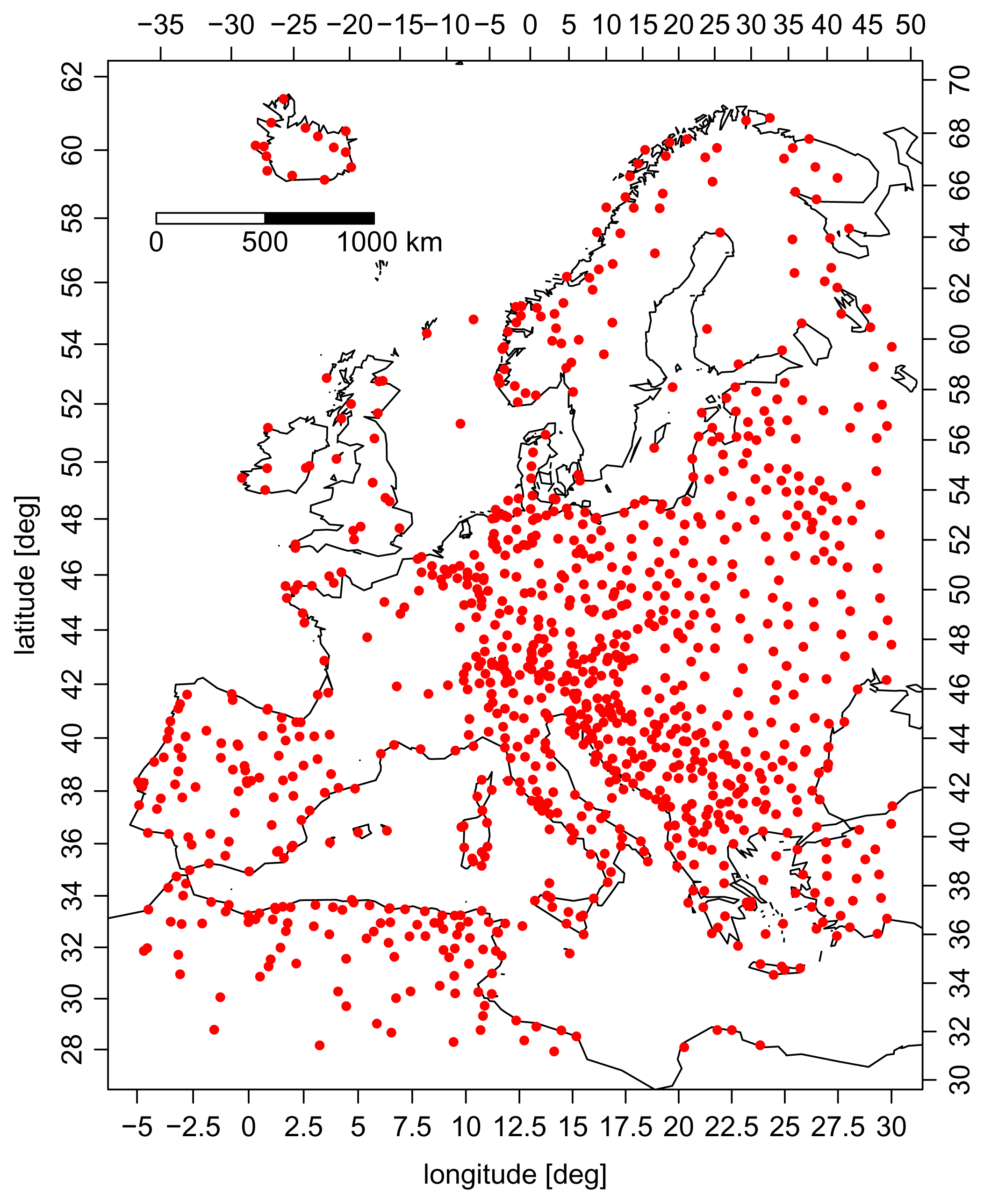
4.2. Meteorological and Ancillary Data

Two sources of meteorological information were used in this study. The first one consists of the SYNOP weather observations from more than 2000 land stations distributed over Europe (Figure 1), which were employed during the algorithm training phase, as well as for the validation purposes. They provide valuable details about the meteorological conditions including cloud coverage and horizontal visibility. Nevertheless, these point observations cannot be easily interpolated to a spatial grid due to the complex nature of cloudiness and visibility distributions [9]. The SYNOP observations are coded according to the scheme described by the WMO [20] and redistributed by the European Centre for Medium-Range Weather Forecasts (ECMWF). Out of this extensive set of synoptic information, the following variables were considered:

• cloud types (at low, middle and high levels).
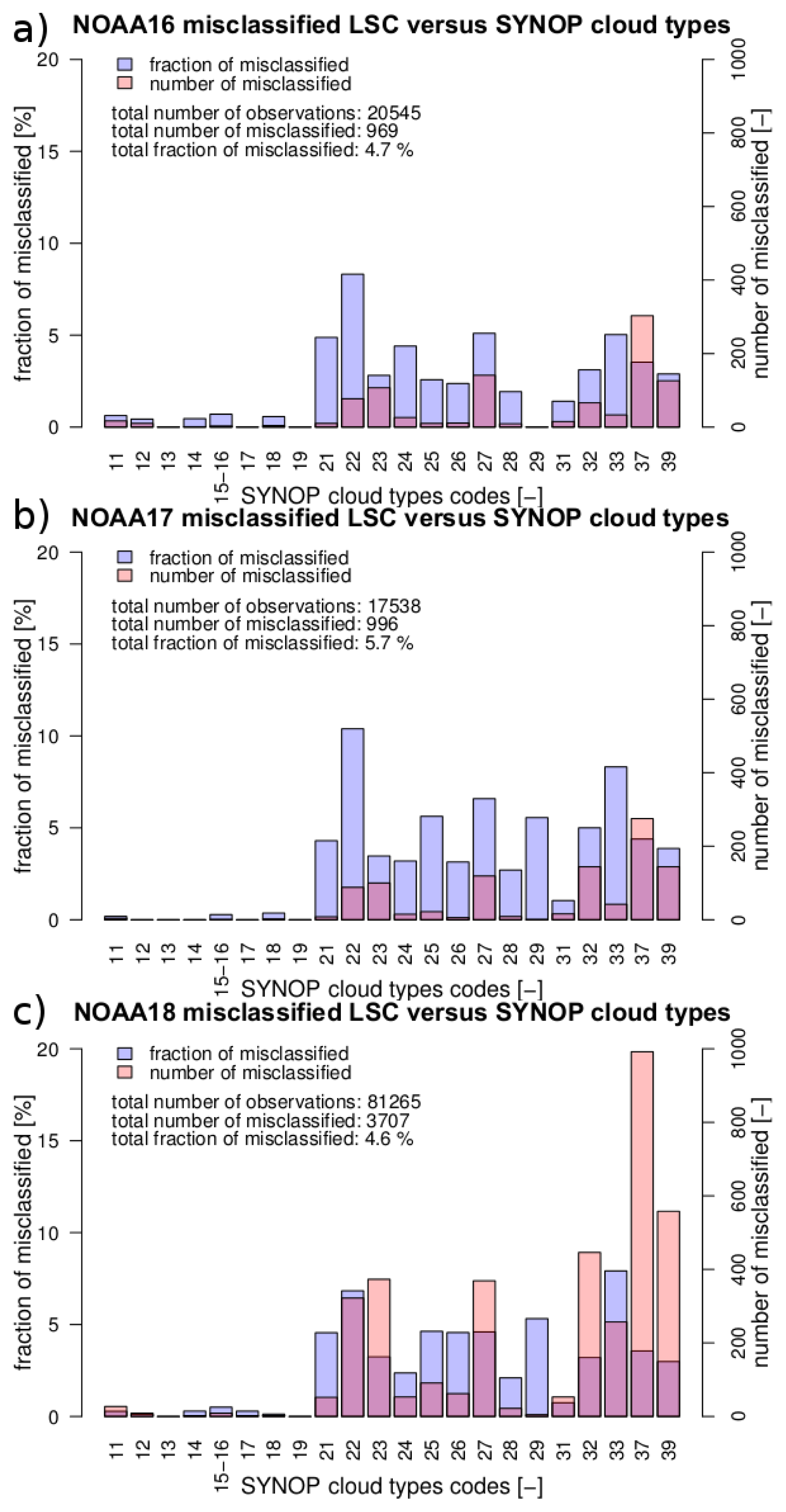
• present weather—coded values describing the current atmospheric conditions. Codes from 10–12 to 40–49 indicate different types of fog events.

The second type of meteorological data employed by the algorithm, consists of the skin surface temperature (SKT) field derived from the ECMWF deterministic forecast model with the three-hour step at 0.2° × 0.2° spatial resolution. Apart from the meteorological data, two DEM datasets provided by the ECMWF (geopotential at the surface) at 0.2° × 0.2° resolution and by the USGS at 1 × 1 km resolution were used to correct SKT estimates over mountainous terrains (see Section 5.3).

5. Methodology of LSC Detection

5.1. Probabilistic Cloud Mask (PCM)

The first step of proposed LSC detection algorithm incorporates utilisation of the probabilistic cloud mask (PCM) method [49] to delineate spectral signature of clouds; therefore, a brief description as an introduction follows. PCM is based on the multidimensional LUT, where classification probability estimates between clear-sky, cloudy and snow categories are stored. Each dimension consists of discrete information related to: satellite measurements, acquisition angles, land cover, and surface temperature. In order to transform a continuous dataset (e.g., satellite measurements) to a discrete form, its values are located within several binning thresholds by means of the Approximate Nearest Neighbour (ANN) technique [50]. One of the novel features of the PCM method is utilisation of the Invariant Coordinate System (ICS) transformation [51], which is employed to enhance spectral contrast of thin and broken clouds. The algorithm is trained against PPS cloud mask version 2012 [45] and MODIS snow mask collection 5 [52]. The image classification process involves application of the ICS technique and localisation of input datasets within the LUT by means of the ANN method. In this way, probability estimates are extracted from the LUT and acquired results are further post-processed to derive a binary dataset using probability threshold values. This product is further used in the proposed algorithm to discriminate cloud cover.

5.2. Algorithm Design

The proposed methodology of LSC detection stems from the collocated AVHRR/SYNOP observations that are utilised to separate the LSC spectral signature amongst other cloud types. This information is further employed during the algorithm training phase to construct two look-up vectors (LUVs) containing the precomputed probability estimates (separately suited for the 1.6/3.7 μm channel configurations). The classification process considers only pixels marked as overcast by the PCM cloud mask [48] and is limited to localisation of input data within the LUV composed of a bitwise combination of six features:

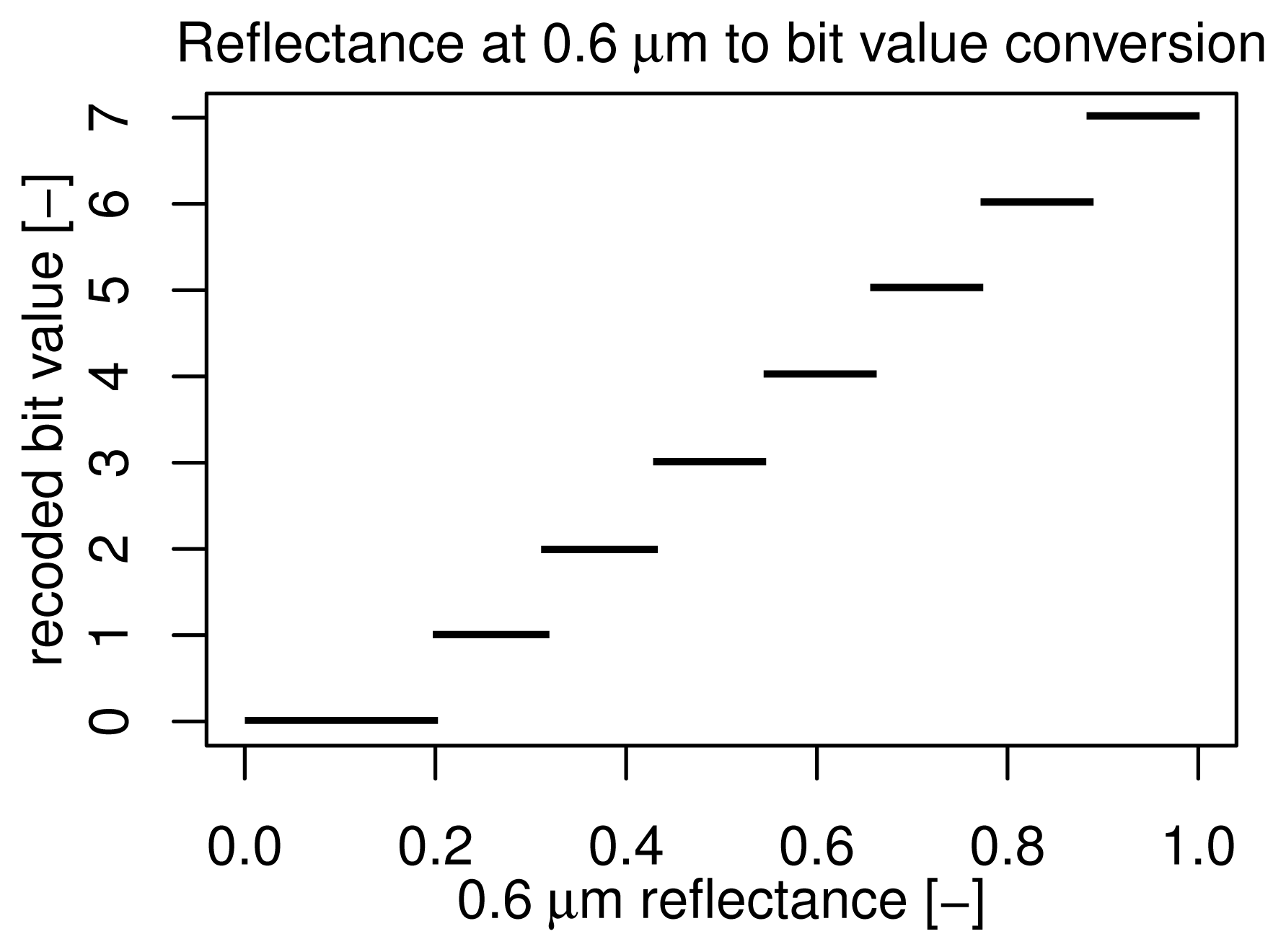
• 0.6 μm reflectance which contains information about the cloud optical depth.
• 1.6/3.7 μm reflectance which contains information about the cloud droplet radius.
• 10.8 μm BT which contains information about the thermodynamic state of a cloud.
• SKT-10.8 μm temperature difference which contains information about the cloud height.
• 10.8–12.0 μm BTD which indicates the presence of upper-level cloudiness.
• broken cloudiness flag (described in Section 5.3).

In order to combine continuous values of these features into a single vector they first have to be converted into integer representation F by means of the step functions (Figure 2). Such an approach allows specifying multiple binning values per feature, thereby offering great flexibility over the decision-tree approaches, where usually a single value suited for the instantaneous environmental conditions has to be selected. For each feature, a separate set of coefficients was empirically derived:

$$F_{brk}=\lfloor 0.3\times brk\rfloor$$

(1)

$$F_{0.6}=\lfloor 8.75\times re{f}_{0.6}-0.75\rfloor$$

(2)

$$F_{1.6or3.7}=\lfloor 8.75\times re{f}_{1.6or3.7}\rfloor$$

(3)

$$F_{10.8}=\lfloor 0.25\times b{t}_{10.8}-57\rfloor$$

(4)

$$F_{10.8-12.0}=\lfloor (b{t}_{10.8}-b{t}_{12.0})+1\rfloor$$

(5)

$$F_{SKT-10.8}=\lfloor 0.33\times (SKT-b{t}_{10.8})+1\rfloor$$

(6)

where ref_0.6, ref_1.6or3.7 correspond to the reflectance at 0.6, 1.6 or 3.7 μm; bt_10.8 and bt_12.0 denote the BT at 10.8 and 12.0 μm; SKT is the skin surface temperature; brk is the broken cloudiness feature; ⌊ . . . ⌋ denotes function “floor” that maps a real number to the largest previous integer. If the acquired value is not enclosed within the 0 to 2ⁿ−1 range, then it is set either to 0 if it is negative or to 2ⁿ−1 if it exceeds this value. For features: F_brk, n = 1; F_10.8−12.0, n = 2; F_0.6, F_1.6or3.7, F_SKT−10.8, n = 3; F_10.8, n = 4, which gives a total of 2¹⁶ possibilities.

Preceding the algorithm training phase, a pre-selection of collocated SYNOP/AVHRR observations was performed in order to distinguish unambiguous occurrences of the single-layered LSC cover. This step is crucial for the final classification accuracy as the satellite measurements may not directly correspond to the LSC cover reported by an observer at the ground in case of the multi-layered clouds. In such a situation, the algorithm would be trained against the spectral signature of higher, overlaying clouds and the overall LSC detection skills would deteriorate. Therefore, a presence of the single-layered LSC cover is assumed under the following conditions:

• SYNOP report indicates presence of the LSC.
• SYNOP report indicates absence of middle or high clouds (in case they could be visible through the inhomogeneous LSC cover).
• Thermal contrast between the 10.8 μm cloud top BT and the SKT does not exceed 18 K. This roughly corresponds to the cloud top height at 3 km assuming the temperature lapse rate of 0.6 K/100 m.
• 10.8 μm BT has to be greater than 232 K to exclude thick homogeneous cirrus clouds [53].
• 10.8–12.0 μm BTD has to be lower than 1 K to exclude high clouds.
• 0.6 μm reflectance has to be greater than 0.2 to exclude clouds with small optical thickness such as cirrus [54].

If one of those conditions is not met, then the collocated AVHRR/SYNOP observation is treated as a non-LSC case during the algorithm training and validation processes.

5.3. Preparation of Input Data

At the first step of the algorithm, all satellite datasets were remapped into the Lambert Equal Area (LAEA) projection that preserves ground pixel size and is thus suitable for spatial analyses. Furthermore, the SKT dataset was linearly interpolated between two forecast model time steps in order to match satellite acquisition time. These estimates together with the DEM were bilinearly interpolated from the 0.2° × 0.2° ECMWF grid to the 1 × 1 km LAEA projection. However, the upscaled SKT dataset does not resolve well small-scale temperature variations over rough topography. Thus, a simple temperature correction was employed on the basis of altitude difference between the upscaled ECMWF DEM and the 1 × 1 km USGS DEM multiplied by the temperature lapse rate of 0.6 K/100 m.

$$\mathbf{K}=\left[\begin{array}{ccccc}-\frac{1}{24}& -\frac{1}{24}& -\frac{1}{24}& -\frac{1}{24}& -\frac{1}{24}\\ -\frac{1}{24}& -\frac{1}{24}& -\frac{1}{24}& -\frac{1}{24}& -\frac{1}{24}\\ -\frac{1}{24}& -\frac{1}{24}& 1& -\frac{1}{24}& -\frac{1}{24}\\ -\frac{1}{24}& -\frac{1}{24}& -\frac{1}{24}& -\frac{1}{24}& -\frac{1}{24}\\ -\frac{1}{24}& -\frac{1}{24}& -\frac{1}{24}& -\frac{1}{24}& -\frac{1}{24}\end{array}\right]$$

(7)

Moreover, on the basis of binary PCM cloud mask (Figure 3a), broken clouds were discriminated by means of the double kernel convolution process. At the beginning, the cloud mask was convolved with the 5 × 5 kernel presented in the Equation (7). The acquired positive values (Figure 3b) for every pixel located near the cloud edge are related to the number of overcast pixels within the kernel window. High, positive values indicate an inhomogeneous sky with highly separated cloudiness. Conversely, zero or negative values are related either to clear-sky or fully overcast conditions. In order to exclude pixels located at the edges of vast homogeneous clouds, the positive values were used to mask (set to 0) pixels from the PCM cloud mask. This modified dataset was then convolved with the 7 × 7 kernel window composed of the value 1 (Figure 3c). The acquired positive values were further utilised to mask pixels from the previous convolution process (i.e., Figure 3b). The final result consists of a mask of broken cloudiness with values ranging between 0 and 100 (Figure 3d).

At the next step of the data preparation process, the SYNOP weather reports were collocated with the remapped satellite data in space and time domains. The maximum allowed time difference between a ground observation and a satellite overpass was set to 15 min. Furthermore, from the input datasets, only cloudy pixels were selected by means of the PCM cloud mask, and they were averaged within the 3 km radius around each SYNOP station. Some tests were performed with a larger 30 km radius (results not shown); however, the obtained results were of inferior quality. The reason for this may be related to fusion of spectral signatures from different cloud types within a larger search window. Finally, all of the collocated SYNOP observations, AVHRR measurements, PPS cloud type, broken cloudiness masks and SKT estimates extracted from cloudy pixels were divided between training and validation data.

5.4. Algorithm Training Phase

The algorithm training was performed on the basis of 70% of initially collocated SYNOP/NOAA16,18 observations (after [55]) and 90% of SYNOP/NOAA17 observations (due to a small amount of collocations for this platform). Then to the training data a set of functions (Equations (1)–(6)) was applied in order to transform continuous estimates to a discrete form. Acquired integer values were combined into a single feature which represents a unique combination of all input datasets. This was achieved by bitwise shifting and alternation (OR operator) which were performed in the specific order. First, the broken cloudiness flag F_brk was used as an initial value that occupies the least important first bit. Then, the F_SKT−10.8 values were shifted by a one-bit position and merged with the outcomes of F_brk by means of the OR operator. Consequently, the F_10.8−12.0 values were shifted by four-bit positions and merged with data from the previous steps. The same process was repeated for the remaining features in the following order: F_10.8, F_1.6or3.7 and F_0.6. The entire bitwise processing can be expressed by Equation (8). On the basis of combined data, a histogram was computed with bins located around each integer from the 0 to 2¹⁶ −1 range. This corresponds to the minimum and maximum values that could be obtained from the bitwise operations. As a consequence, a single vector V_all is derived, containing occurrence frequency of a particular unique combination of the six features within the training dataset.

$$V_{all}=(((((F_{brk}\hspace{0.17em}OR\hspace{0.17em}{F}_{SKT-10.8}\times 2)\hspace{0.17em}OR\hspace{0.17em}{F}_{10.8-12.0}\times 2^4)\hspace{0.17em}OR\hspace{0.17em}{F}_{10.8}\times 2^6)\hspace{0.17em}OR\hspace{0.17em}{F}_{1.6or3.7}\times 2^{10})\hspace{0.17em}OR\hspace{0.17em}{F}_{0.6}\times 2^{13})$$

(8)

The second stage of the training process was performed analogically to the previous one, but only for the collocated observations where an observer at a SYNOP station reported the LSC occurrence. As a result, the second 2¹⁶ element vector V_LSC was derived. It was further divided by the V_all vector element by element, producing a third vector LUV_prob with the LSC probability estimates (Equation (9)), where each element specifies the ratio between the number of LSC occurrences and the total number of observations for a particular bitwise combination of the selected features. For the elements where input data did not comply to the restrictions listed in Subsection 5.2, the LSC probability was prescribed to 0. Finally, the acquired results were stored as two separate look-up vectors (LUVs) depending on the 1.6/3.7 μm AVHRR channel configuration.

$$LU{V}_{prob}=\frac{V_{LSC}}{V_{all}}$$

(9)

5.5. Algorithm Validation and Derivation of LSC Data

Validation of the proposed algorithm was performed on 30% of the collocated NOAA16,18 observations and on 10% of the NOAA17 observations, which were not used for the algorithm training. In the beginning, selected features (Equations (1)–(6)) were combined into a single one by means of the bitwise operations analogically to the training phase (Equation (8)). Acquired bit representation corresponds to a unique position in the LUV and can be directly used as a vector index to extract the LSC probability values. These estimates were further transformed to a binary mask assuming LSC occurrence above the 50% probability threshold. Then the contingency matrices (Equation (10)) for the proposed algorithm and for the PPS cloud-type products were derived by collation with the SYNOP data and the following classification quality indicators were computed (Equations (11)–(17)): Probability Of Detection (POD), False Alarm Rate (FAR) for LSC and other cloud types, Bias, Hit Rate (HR) and Hanssen–Kuipers Skill Score (KSS). Analogous validation analysis was performed for the SYNOP stations located within the 20 km distance from a shoreline in order to assess the maritime stratus detection accuracy.

$$\begin{array}{ccc}counts& AVHRR\hspace{0.17em}other& AVHRR\hspace{0.17em}LSC\\ SYNOP\hspace{0.17em}other& a& b\\ SYNOP\hspace{0.17em}LSC& c& d\end{array}$$

(10)

$$PO{D}_{LSC}=\frac{d}{c+d}$$

(11)

$$PO{D}_{other}=\frac{a}{a+b}$$

(12)

$$FA{R}_{LSC}=\frac{b}{b+d}$$

(13)

$$FA{R}_{other}=\frac{c}{a+c}$$

(14)

$$BIAS=\frac{d+c}{d+b}$$

(15)

$$HR=\frac{a+d}{a+b+c+d},\mathrm{\hspace{0.17em} }\mathrm{\hspace{0.17em} }\mathrm{\hspace{0.17em} }\text{where\hspace{0.17em}}0\le HR\le 1$$

(16)

$$KSS=\frac{a\times d-c\times b}{(a+b)\times (c+d)},\mathrm{\hspace{0.17em} }\mathrm{\hspace{0.17em} }\text{where}-1\le KSS\le 1$$

(17)

Ultimately, the LSC spatial estimates were derived over the selected European region by means of the proposed algorithm. This involved the same procedure as in the case of the validation process, where initially the step functions were applied to the input data; secondly, the integer representations of features were combined by bitwise operations, and finally, the acquired values were used as indexes to extract probability estimates from the LUV. In this manner, scenes acquired by the NOAA17,18 satellites in the year 2008 and by the NOAA16 in 2011 were processed. An example of the final LSC probability product is presented in Figure 4.

6. Discussion of Acquired Results

Accuracy assessment of the proposed methodology involved spatial and temporal analyses of the LSC probability distribution over Europe, comparison with the PPS cloud-type product and validation against the SYNOP reports. However, while interpreting these results, it has to be emphasised that they refer to the LSC cover not overlaid by higher clouds as defined by constraints presented in Section 5.4. From the collocated SYNOP/AVHRR observations, it was determined that only 24% of LSC observations comply to these restrictions. This issue was also discussed by [56], who compared low-level cloudiness derived from the International Satellite Cloud Climatology Project (ISCCP) with global SYNOP cloudiness data over land and ocean compiled by [57]. We are found that ISCCP mean estimates in comparison to [57] are up to 40% lower and they feature a distinct annual cycle not evident in the latter dataset. We are justified these results, arguing that low-level cloud fraction estimated from satellite data depends not only on clouds in the lower atmosphere, but also on the clouds above. More recently, [58] found that 44% of global cloud cover retrieved from the CALIOP LIDAR measurements is composed of more than one layer. On the basis of European SYNOP data utilised in this study, it was determined that in 48% of all cases a low-level cloud (codes 31–39) was reported alongside a higher one (codes 11–19 and 21–29). To recapitulate the influence of multi-layered cloudiness, it has to be emphasised that the frequency and magnitude of LSC cover acquired in this study is not meant to correspond well with the real climatological values.

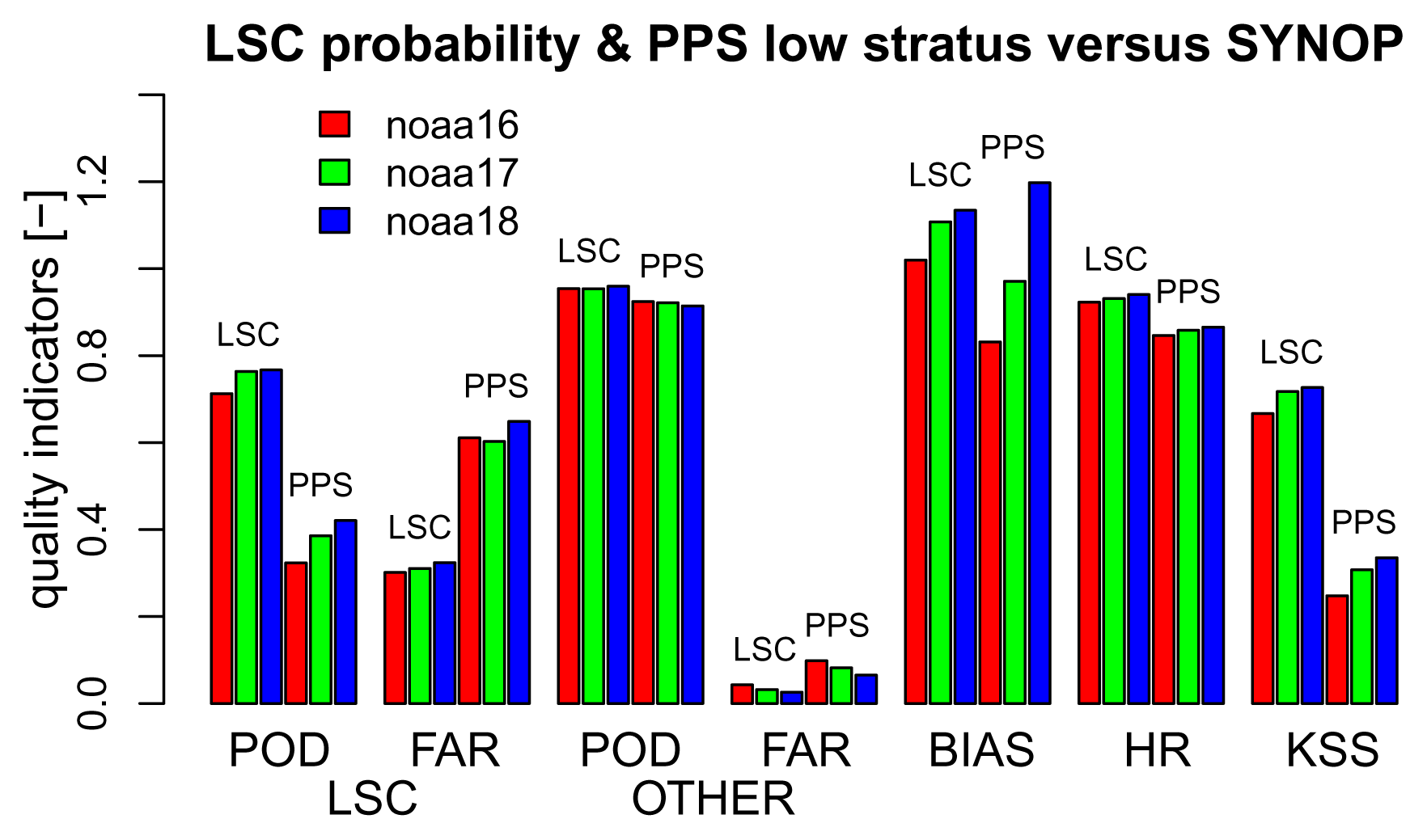
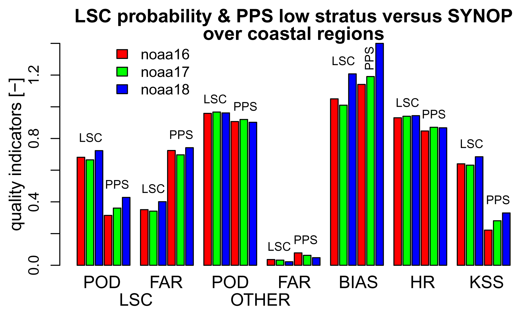
6.1. Validation against SYNOP Observations

Preceding the validation of the proposed algorithm, the low-level cloudiness detection accuracy of the input PCM cloud mask was determined from the comparison with SYNOP data. It occurred that the POD for LSC amongst other cloud types reaches 0.92, 0.95, 0.96 for the NOAA16,17,18 platforms, respectively. This implies that the accuracy of PCM cloud mask does not significantly affect the overall LSC detection skills. However, they are influenced by misclassified or erroneously coded cloud-type observations incorporated in the SYNOP reports that are difficult to identify.

The LSC mask derived by means of the proposed algorithm was validated together with the PPS cloud-type product [45] against the SYNOP observations for the sake of comparison with other well-established methods. LSC cover from the PPS data was determined as a combination of classes: “Very low stratiform cloud” and “Low stratiform cloud.” Computed quality indicators (Figure 5) retrieved from the collocated SYNOP/LSC data proved good detection skills of the proposed method and inferior accuracy of the PPS cloud-type product. The fraction of correctly detected LSC events (POD_LSC) as compared to the SYNOP reports equals around 74% for the proposed algorithm and 40% for the PPS product. The LSC occurrences not detected by the PPS algorithm contributes to the fraction of other misclassified cloud types (FAR_other), which is significantly greater for the PPS than in the case of the proposed algorithm. A high fraction of correctly identified non-LSC cases (POD_other) and a high fraction of hits as compared to a total number of samples (HR) for both analysed algorithms are related to an unbalanced contingency table. It contains 76% less LSC occurrences than in a true climatological value due to the multi-layered cloud formations. Consequently, the term “a” in the contingency table has by far the greatest value, rendering the numerator and denominator in Equations (12) and (16) almost equal. In such a case, the KSS value expresses objective LSC detection skills, clearly indicating better performance of the proposed algorithm (KSS ~ 0.70) in comparison to the PPS cloud-type product (KSS ~ 0.38). Regarding the differences in validation scores between satellites, they are small for both analysed algorithms with slightly worse results for the NOAA16 platform, which could be associated with the least favourable illumination conditions (high SZA) for this satellite and a different time frame of analysis. However, the Bias values for PPS product are quite variable and they indicate that the NOAA16 LSC occurrence frequency is underestimated, whereas the reverse pattern is related to the NOAA18 platform. Concerning the proposed algorithm, these discrepancies are smaller and the Bias revealed slight overestimation of the LSC occurrence frequency.

As mentioned in Section 2.2, spectral properties of the maritime stratus are slightly different than its land equivalent due to the lower concentration of CCN [32]. Therefore, to analyse the influence of this difference on the accuracies of selected algorithms, the validation analysis was performed once more only for the SYNOP stations located within the 20 km distance from a shoreline (Figure 6). It occurred that the acquired results are slightly inferior to the validation against all SYNOP stations for both algorithms. This may indicate that the spectral properties of maritime stratus are more similar to other cloud types, especially to altostratus [59]. As a result there is too much ambiguity to differentiate between them. Another reason might be related to lower accuracy of the up-scaled SKT data over coastal regions, which is the result of bi-linear interpolation of coarse resolution NWP data. However, the discrepancies in quality scores between land and oceanic regions do not preclude utilisation of the proposed method for the maritime LSC discrimination.

Overall accuracy of the proposed algorithm expressed by the KSS value is reduced by relatively high FAR_LSC. Therefore, additional analysis was performed in order to determine which cloud types are most frequently confused with the LSC cover. For each cloud type listed in Table 1, the number of misclassified cases was computed together with the fraction which they comprise in comparison to the total number of occurrences. For high clouds (codes 11–19) only cases when the observer did not report the lower ones were considered. Acquired results presented in Figure 7 clearly indicate that the applied constraints correctly excluded high-level cloudiness which are rarely classified as LSC.

Relative to the occurrence frequency (blue bars in Figure 7), the most ambiguous for the correct LSC discrimination are optically thick-cloud types such as altostratus opacus/nimbostratus (code 22); altocumulus translucidus or opacus, or altocumulus opacus in a single layer (code 27); cumulonimbus calvus, with or without cumulus, stratocumulus or stratus (code 33). From the quantitative perspective, it could be seen that the most frequently misclassified (red bars in Figure 7) are low-level clouds that well comply with the restrictions listed in Section 5.4. This analysis showed that the discrimination between LSC and other middle and low clouds is sometimes impossible, as from the satellite perspective they feature the same spectral characteristics, while an observer at the ground level is able to perceive their different base heights and macroscopic properties. Therefore, these limitations have to be taken into account while interpreting the presented results.

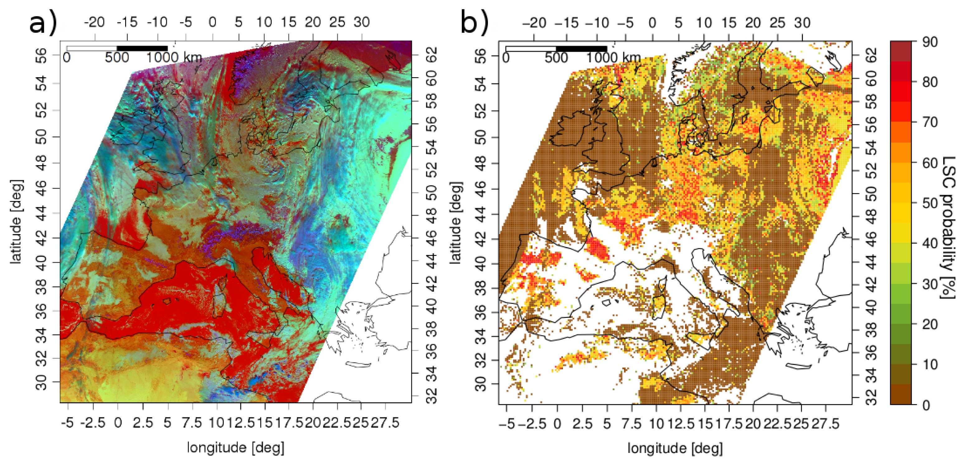
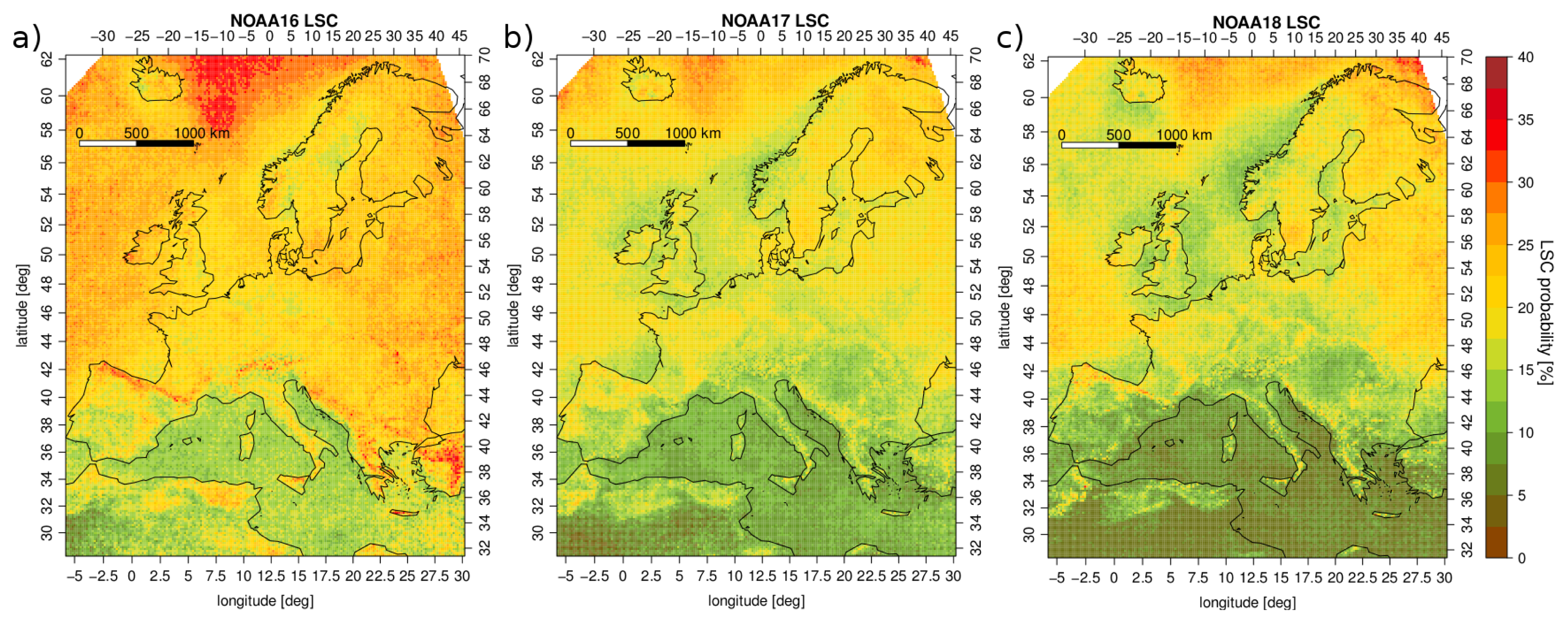
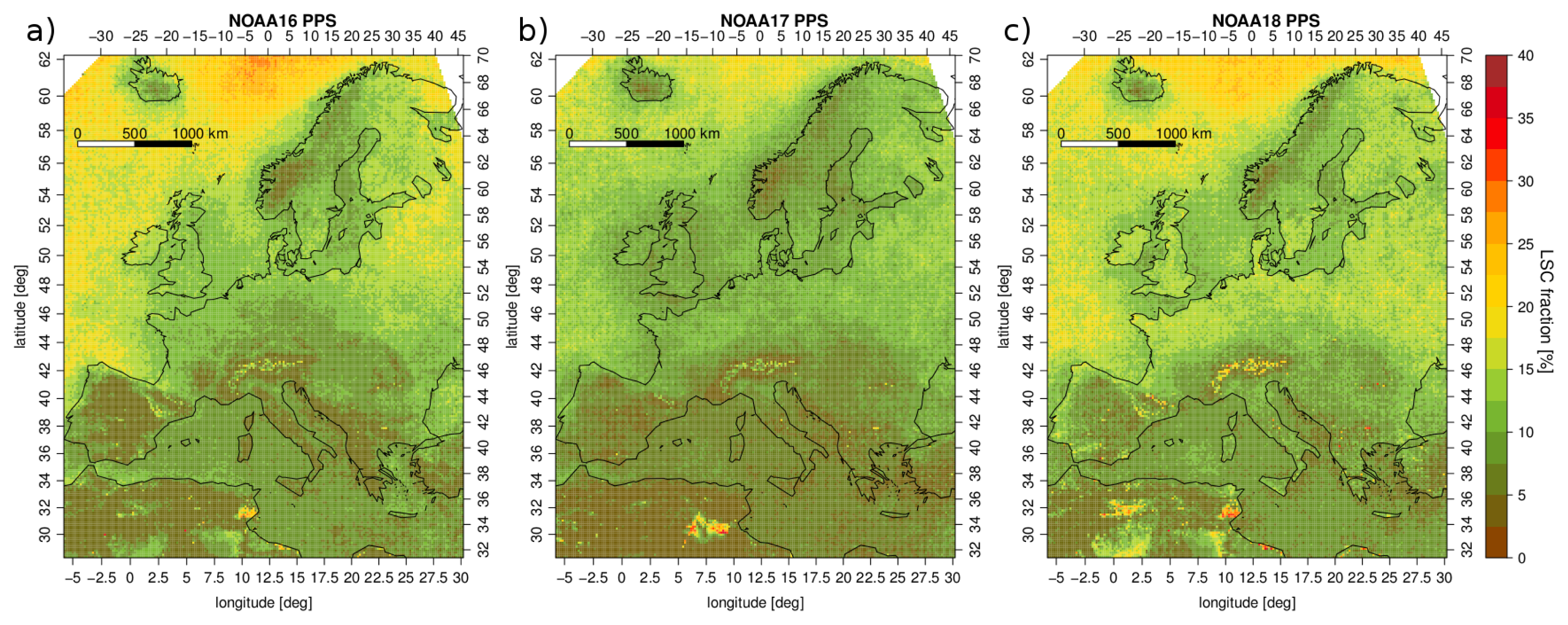
6.2. Spatial Distribution of LSC over Europe

Spatial patterns of the LSC occurrence were investigated on mean annual composites (Figures 8 and 9) covering the year 2008 for the platforms NOAA17,18, and the year 2011 for the platform NOAA16. The analyses were performed for the LSC probability and for the PPS LSC fraction (retrieved from the cloud type product). In theory they should stay in good agreement because the proposed algorithm describes probability as the ratio between the number of LSC occurrences and the total number of cases, which over a long time frame, corresponds well with the cloud fraction. However, in practise, the acquired results indicate that the PPS LSC fraction has significantly lower values than the LSC probability product. From the spatial perspective, both algorithms reported higher cloudiness over the Atlantic Ocean than over the Mediterranean Sea; however, over land, the LSC occurrence latitudinal gradient is less apparent in the PPS data, while the LSC probability increases in the northeastern direction. Over North Africa, the LSC product reports higher probability over the coastal region, where low clouds form during the night and remain in the morning. Conversely, in the PPS product, they are not apparent as opposed to other deserted areas which are misclassified as clouds [48]. All of the aforementioned issues adversely influence the PPS LSC discrimination accuracy which was assessed during the validation analysis (Figure 5).

Concerning the LSC probability (Figure 8), it could be easily noticed that the highest values correspond to NOAA16 satellite and the lowest to NOAA18 platform. This issue is related to the satellite overpass time (over Europe) which for NOAA16,17 platforms falls during the morning and evening hours, while for NOAA18 it falls around midday and midnight. Thus, the acquired imagery corresponds to different parts of the LSC diurnal cycle which has its minimum during the daytime. On the contrary, higher level clouds develop more efficiently during the day due to the convective processes; their maximal diurnal frequency thus overlaps with the minimum of the LSC cycle. Hence, the differences between morning and afternoon polar orbiting satellites are even more pronounced. In order to confirm this hypothesis, the annual distributions of mean hourly fractions of LSC, middle and high clouds in 2008 were derived from the SYNOP data and compared to the corresponding mean LSC probability estimates retrieved from AVHRR data (Figure 10). It occurred that SYNOP reports and AVHRR retrievals follow the same temporal pattern of the LSC cycle with different magnitudes.

On this basis it is evident that NOAA18 platform acquires data during the daily minimum of LSC cycle and the daily maximum of high-clouds cycle which corresponds well with the pattern revealed by the obtained results. Moreover, they are consistent with the findings of [60] who developed a cloud classification algorithm suited for data from the spaceborne Cloud Profiling Radar (CPR) mounted aboard the CloudSat platform. The CPR instrument provides a unique information on the atmospheric vertical profile of clouds due to the characteristics of 94 GHz radiation, which is able to penetrate through thick clouds down to the surface. This in turn allows for accurately discriminating low clouds which were further classified by [60] into the joined Stratus (St) and Stratocumulus (Sc) category. For the period from June 2006 to June 2007 they derived the 2.5° × 2.5° mean St & Sc fraction, which is consistent with the LSC probability estimates acquired in this study from the spatial and qualitative perspectives. The overpass time of CloudSat satellite is similar to the NOAA18 platform; thus over Europe it corresponds to the diurnal minimum of LSC occurrence. The acquired mean annual LSC probability composites were further compared to the annual LSC fraction computed for each SYNOP station (Figure 11). It occurred that differences between these two datasets are high possibly due to the multi-layered cloud formations. They might be also the reason for different spatial patterns of the LSC occurrence which for the station data exhibit an increase in the east–west direction. The reverse pattern is apparent on the mean annual LSC composites (Figure 8) possibly due to the higher frequency of low-pressure systems with multi-layered cloud formations occurring in the oceanic climate of Western Europe. They are less frequent over the eastern parts with a more continental climate; the single-layered LSC cases are thus more common. Nevertheless, to prove this hypothesis, a more detailed analysis based on blended CALIOP and CPR data is needed.

6.3. Spatio-Temporal Distribution of LSC over Europe

At the next step of analysis, spatial and temporal aspects of the latitudinal LSC probability distribution across Europe over the course of selected years were investigated (Figure 12). The acquired results indicate a presence of the annual LSC probability cycle with the lowest values for the NOAA18 platform. However, the cycle is only well pronounced over the latitude range between 40° and 60°, where the LSC probability is significantly lower for the summer months from the beginning of May until the end of August. This period is consistent with the findings of [61] who investigated monthly mean fog frequency for a long time series (1901–2012) of synoptic observations collected at the Zürich/Fluntern weather stations in Switzerland. Mean LSC probability for the latitudes below 40° is lower than 7.5% and the annual variations are small. On the other hand, for latitudes greater than 60° the LSC cover is persistent (>15%) over the course of the year. Nevertheless, it should be emphasised that these results correspond to daytime data only and they are influenced by unequal distribution of land and water surfaces over the selected region. This implies that for higher latitudes, most of the signal originates from ocean surfaces where low-level cloudiness is predominant. On the contrary, the latitudinal range between 40° and 60° corresponds mainly to the land surfaces, where convection processes are more pronounced during a warmer part of the year. This leads to unstable atmospheric conditions which are unfavourable for the LSC formation.

7. Conclusions

In this study, a novel method for the daytime low stratiform clouds (LSC) detection on Advanced Very High Resolution Radiometer (AVHRR) imagery was presented. Its unique feature is related to estimation of LSC occurrence probability based on satellite spectral information and simulated skin surface temperature. Such an approach allows specification of different confidence intervals which expands the usability of binary output provided by various contemporary algorithms. The proposed methodology stems from the collocated synoptic (SYNOP) cloud-type reports and AVHRR measurements that were employed to train and validate the algorithm. However, direct utilisation of the collocated data is limited due to the multi-layered cloud formations, where the spectral signature of LSC is masked or modified by overlaying clouds. In order to discriminate such situations, the following set of constraints was applied:

• Within the SYNOP reports, LSC cannot be identified together with middle and/or high clouds.

When higher clouds are invisible through the homogeneous LSC cover, the constraints based on satellite data are applied:

• Thermal contrast between the 10.8 μm cloud top brightness temperature (BT) and skin surface temperature retrieved from a climate model cannot exceed 18 K.
• 10.8 μm BT has to be greater than 232 K.
• 10.8–12.0 μm BT difference has to be lower than 1 K.
• 0.6 μm reflectance has to be greater than 0.2.

The satellite image classification process is based on six features that are initially converted to the integer form by step functions and combined by means of bitwise operations. As a result, a set of values reflecting the unique combination of six features is derived which is further employed to extract LSC occurrence probability estimates from the precomputed look-up vectors (LUVs). The acquired product consists of continuous probability estimates that can be transformed to a binary form, assuming the LSC presence above the threshold of 50%. Performed analyses revealed a diurnal probability cycle, where the NOAA16,17 satellites with morning overpass time reported higher values than the midday NOAA18 platform. Moreover, the study of spatio-temporal pattern revealed the existence of the annual cycle, which is mostly apparent for the latitudinal range between 40° and 60° . During the validation analysis quality indicators confirmed good accuracy of the proposed LSC detection algorithm (KSS > 0.6) and inferior accuracy of the reference PPS method (KSS > 0.4). In some of the cases, the LSC presence was erroneously assigned to other cloud types. This issue was further analysed and it occurred that the most frequently misclassified objects are low-level clouds, whereas single-layered high clouds are rarely confused with the LSC. Considering the total fraction of misclassified cases within a particular cloud type, it was found that the most dubious cases for correct LSC discrimination are: altostratus opacus, nimbostratus, altocumulus translucidus or opacus, cumulonimbus calvus, with or without cumulus. On this basis it was concluded that without the cloud-base altitude estimates and macroscopic properties apparent to an observer at the ground level, there is no possibility when relying solely on data acquired by passive satellite radiometers, to distinguish between LSC and other optically thick middle and low clouds. Although the classification accuracy of the proposed LSC detection algorithm for nowcasting purposes was proven during the validation against instantaneous SYNOP observations, in the context of operational weather analysis, the usability of the derived product is still to be determined. This should be further assessed by an expert at a weather station who is the main target of the LSC product. Future development of the algorithm will involve expansion of the training dataset beyond the European region and utilisation of satellite data acquired by early generations of the AVHRR instrument.

References

1. Jacobs, W.; Nietosvaara, V.; Bott, A.; Bendix, J.; Cermak, J.; Michaelides, S.; Gultepe, I. Microphysical data of fog observed in Clermont-Ferrand and corresponding satellite images. Short range forecasting methods of fog, visibility and low clouds. COST Action 2008, 722, 2–11. [Google Scholar]
2. Guo, F.; Gu, W.; Yuan, F. Real-time risk assessment model of freeway traffic in rain and fog weather. Appl. Mech. Mater 2012, 226, 2370–2375. [Google Scholar]
3. Cools, M.; Moons, E.; Wets, G. Assessing the impact of weather on traffic intensity. Wea. Clim. Soc 2010, 2, 60–68. [Google Scholar]
4. Gultepe, I.; Pearson, G.; Milbrandt, J.; Hansen, B.; Platnick, S.; Taylor, P.; Gordon, M.; Oakley, J.; Cober, S. The fog remote sensing and modeling field project. Bull. Am. Meteorol. Soc 2009, 90, 341–359. [Google Scholar]
5. Bendix, J. A satellite-based climatology of fog and low-level stratus in Germany and adjacent areas. Atmos. Res 2002, 64, 3–18. [Google Scholar]
6. Błaś, M.; Polkowska, Ż.; Sobik, M.; Klimaszewska, K.; Nowiński, K.; Namieśnik, J. Fog water chemical composition in different geographic regions of Poland. Atmos. Res 2010, 95, 455–469. [Google Scholar]
7. Gultepe, I.; Tardif, R.; Michaelides, S.; Cermak, J.; Bott, A.; Bendix, J.; Müller, M.; Pagowski, M.; Hansen, B.; Ellrod, G.; et al. Fog research: A review of past achievements and future perspectives. Pure Appl. Geophys 2007, 164, 1121–1159. [Google Scholar]
8. Vautard, R.; Yiou, P.; van Oldenborgh, G.J. Decline of fog, mist and haze in Europe over the past 30 years. Nat. Geosci 2009, 2, 115–119. [Google Scholar]
9. Cermak, J.; Bendix, J. Dynamical Nighttime Fog/Low Stratus Detection Based on Meteosat SEVIRI Data: A Feasibility Study. In Fog and Boundary Layer Clouds: Fog Visibility and Forecasting; Springer: Berlin, Germany, 2007; pp. 1179–1192. [Google Scholar]
10. Cermak, J.; Bendix, J. A novel approach to fog/low stratus detection using Meteosat 8 data. Atmos. Res 2008, 87, 279–292. [Google Scholar]
11. Schreiner, A.J.; Ackerman, S.A.; Baum, B.A.; Heidinger, A.K. A multispectral technique for detecting low-level cloudiness near sunrise. J. Atmos. Ocean. Technol 2007, 24, 1800–1810. [Google Scholar]
12. Bendix, J.; Thies, B.; Cermak, J.; Nauß, T. Ground fog detection from space based on MODIS daytime data—A feasibility study. Wea. Forecast 2005, 20, 989–1005. [Google Scholar]
13. WMO, International Cloud Atlas; World Meteorological Organization: Geneva, Switzerland, 1956; p. 62.
14. Houze, R.A., Jr. Cloud Dynamics; Academic Press: Waltham, MA, USA, 1994; Volume 53. [Google Scholar]
15. WMO, International Meteorological Vocabulary; Revised ed; World Meteorological Organization: Geneva, Switzerland, 1986; p. 276.
16. NOAA, Surface Weather Observations and Reports; Office of The Federal Coordinator for Meteorological Services and Supporting Research: Washington, DC, USA, 2005.
17. Welch, R.M.; Wielicki, B.A. The stratocumulus nature of fog. J. Appl. Meteorol 1986, 25, 101–111. [Google Scholar]
18. Allaby, M. Encyclopedia of Weather and Climate, 2nd ed; Facts on File: New York, NY, USA, 2002. [Google Scholar]
19. Klein, S.A.; Hartmann, D.L. The seasonal cycle of low stratiform clouds. J. Clim 1993, 6, 1587–1606. [Google Scholar]
20. WMO, Manual on Codes; Secretariat of the World Meteorological Organization: Geneva, Switzerland, 1995.
21. Cermak, J.; Eastman, R.M.; Bendix, J.; Warren, S.G. European climatology of fog and low stratus based on geostationary satellite observations. Q. J. R. Meteorol. Soc 2009, 135, 2125–2130. [Google Scholar]
22. Bendix, J.; Thies, B.; Nauß, T.; Cermak, J. A feasibility study of daytime fog and low stratus detection with TERRA/AQUA-MODIS over land. Meteorol. Appl 2006, 13, 111–125. [Google Scholar]
23. Gultepe, I.; Milbrandt, J. Microphysical observations and mesoscale model simulation of a warm fog case during FRAM project. Pure Appl. Geophys 2007, 164, 1161–1178. [Google Scholar]
24. Dong, X.; Minnis, P.; Ackerman, T.P.; Clothiaux, E.E.; Mace, G.G.; Long, C.N.; Liljegren, J.C. A 25-month database of stratus cloud properties generated from ground-based measurements at the Atmospheric Radiation Measurement Southern Great Plains Site. J. Geophys. Res. Atmos 2000, 105, 4529–4537. [Google Scholar]
25. Brenguier, J.L.; Pawlowska, H.; Schüller, L.; Preusker, R.; Fischer, J.; Fouquart, Y. Radiative properties of boundary layer clouds: Droplet effective radius versus number concentration. J. Atmos. Sci 2000, 57, 803–821. [Google Scholar]
26. SMHI, Products Validation Report for the SAFNWC/PPS Version 2012; EUMETSAT: Norrköping, Finland, 2012.
27. Allen, R.; Durkee, P.; Wash, C. Snow/cloud discrimination with multispectral satellite measurements. J. Appl. Meteorol 1990, 29, 994–1004. [Google Scholar]
28. Key, J. The Cloud and Surface Parameter Retrieval (CASPR) System for Polar AVHRR: User’s Guide: Version 4.0; University of Wisconsin: Madison, WI, USA, 2002. [Google Scholar]
29. Khlopenkov, K.; Trishchenko, A. SPARC: New cloud, snow, and cloud shadow detection scheme for historical 1-km AVHHR data over Canada. J. Atmos.Ocean. Technol 2007, 24, 322–343. [Google Scholar]
30. Lee, T.F.; Turk, F.J.; Richardson, K. Stratus and fog products using GOES-8-9 3.9-_ m data. Wea. Forecast 1997, 12, 664–677. [Google Scholar]
31. Ackerman, S.; Strabala, K.; Menzel, W.; Frey, R.; Moeller, C.; Gumley, L. Discriminating clear sky from clouds with MODIS. J. Geophys. Res 1998, 103, 32–141. [Google Scholar]
32. Yum, S.S.; Hudson, J.G. Maritime/continental microphysical contrasts in stratus. Tellus 2002, 54, 61–73. [Google Scholar]
33. Eyre, J.; Brownscombe, J.; Allam, R. Detection of fog at night using Advanced Very High Resolution Radiometer (AVHRR) imagery. Meteorol. Mag 1984, 113, 266–271. [Google Scholar]
34. Turner, J.; Allam, R.; Maine, D. A case study of the detection of fog at night using channels 3 and 4 on the Advanced Very High Resolution Radiometer (AVHRR). Meteor. Mag 1986, 115, 285–290. [Google Scholar]
35. Dybbroe, A. Automatic Detection of Fog at Night Using AVHRR Data. Proceedings of the 6th AVHRR Data Users’ Meeting, Belgirate, Italy, 29 June–2 July 1993; pp. 254–252.
36. Chaurasia, S.; Sathiyamoorthy, V.; Paul Shukla, B.; Simon, B.; Joshi, P.; Pal, P. Night time fog detection using MODIS data over Northern India. Meteorol. Appl 2011, 18, 483–494. [Google Scholar]
37. Ellrod, G.P. Advances in the detection and analysis of fog at night using GOES multispectral infrared imagery. Wea. Forecast 1995, 10, 606–619. [Google Scholar]
38. Roebeling, R.; Feijt, A.; Stammes, P. Cloud property retrievals for climate monitoring: Implications of differences between Spinning Enhanced Visible and Infrared Imager (SEVIRI) on METEOSAT-8 and Advanced Very High Resolution Radiometer (AVHRR) on NOAA-17. J. Geophys. Res.: Atmos 2006, 111, 20210–20226. [Google Scholar]
39. Anthis, A.; Cracknell, A. Use of satellite images for fog detection (AVHRR) and forecast of fog dissipation (METEOSAT) over lowland Thessalia, Hellas. Int. J. Remote Sens 1999, 20, 1107–1124. [Google Scholar]
40. Wright, B.; Thomas, N. An objective visibility analysis and very-short-range forecasting system. Meteorol. Appl 1998, 5, 157–181. [Google Scholar]
41. Herzegh, P.; Wiener, G.; Bankert, R.; Benjamin, S.; Bateman, S.; Cowie, J.; Hadjimichael, M.; Tryhane, M.; Weekley, B. Development of FAA National Ceiling and Visibility Products: Challenges, Strategies and Progress. Proceedings of the 12th Conference on Aviation Range and Aerospace Meteorology, Atlanta, GA, USA, 28 January–2 February 2006.
42. Guidard, V.; Tzanos, D. Analysis of fog probability from a combination of satellite and ground observation data. Pure Appl. Geophys 2007, 164, 1207–1220. [Google Scholar]
43. Wind, G.; Platnick, S.; King, M.D.; Hubanks, P.A.; Pavolonis, M.J.; Heidinger, A.K.; Yang, P.; Baum, B.A. Multilayer cloud detection with the MODIS near-infrared water vapor absorption band. J. Appl. Meteorol. Climatol 2010, 49, 2315–2333. [Google Scholar]
44. Yoo, J.M.; Jeong, M.J.; Hur, Y.M.; Shin, D.B. Improved fog detection from satellite in the presence of clouds. Asia-Pac. J. Atmos. Sci 2010, 46, 29–40. [Google Scholar]
45. Dybbroe, A.; Karlsson, K.; Thoss, A. NWCSAF AVHRR cloud detection and analysis using dynamic thresholds and radiative transfer modeling. Part I: Algorithm description. J. Appl. Meteorol 2005, 44, 39–54. [Google Scholar]
46. Hüsler, F.; Fontana, F.; Neuhaus, C.; Riffler, M.; Musial, J.; Wunderle, S. AVHRR archive and processing facility at the University of Bern: A comprehensive 1-km satellite data set for climate change studies. EARSeL eProc 2011, 10, 83–101. [Google Scholar]
47. Brunel, P.; Marsouin, A. Operational AVHRR navigation results. Int. J. Remote Sens 2000, 21, 951–972. [Google Scholar]
48. Musial, J.; Hüsler, F.; Sütterlin, M.; Neuhaus, C.; Wunderle, S. Probabilistic approach to cloud and snow detection on Advanced Very High Resolution Radiometer (AVHRR) imagery. Atmos. Meas. Tech 2014, 7, 799–822. [Google Scholar]
49. Musial, J.; Hüsler, F.; Sütterlin, M.; Neuhaus, C.; Wunderle, S. Probabilistic approach to cloud and snow detection on AVHRR imagery. Atmos. Meas. Tech. Discuss 2013, 6, 8445–8507. [Google Scholar]
50. Arya, S.; Mount, D.; Netanyahu, N.; Silverman, R.; Wu, A. An optimal algorithm for approximate nearest neighbor searching fixed dimensions. J. ACM 1998, 45, 891–923. [Google Scholar]
51. Tyler, D.E.; Critchley, F.; Dümbgen, L.; Oja, H. Invariant co-ordinate selection. J. R. Stat. Soc.: Ser. B (Stat. Methodol.) 2009, 71, 549–592. [Google Scholar]
52. Hall, D.; Riggs, G.; Salomonson, V.; DiGirolamo, N.; Bayr, K. MODIS snow-cover products. Remote Sens. Environ 2002, 83, 181–194. [Google Scholar]
53. Ou, S.; Liou, K.; Baum, B. Detection of multilayer cirrus cloud systems using AVHRR data: Verification based on FIRE-II-IF0 composite measurements. J. Appl. Meteorol 1996, 35, 178–191. [Google Scholar]
54. Minnis, P.; Alvarez, J.; Young, D.; Sassen, K.; Grund, C. The 27-28 October 1986 FIRE IFO cirrus case study—Cirrus parameter relationships derived from satellite and lidar data. Mon. Wea. Rev 1990, 118, 2402–2425. [Google Scholar]
55. Miller, A. Subset Selection in Regression; CRC Press: Boca Raton, FL, USA, 2002. [Google Scholar]
56. Weare, B.C. Near-global observations of low clouds. J. Clim 2000, 13, 1255–1268. [Google Scholar]
57. Hahn, C.J.; Warren, S.G.; London, J. Edited Synoptic Cloud Reports from Ships and Land Stations Over the Globe, 1982–1991; Technical report; Carbon Dioxide Information Analysis Center, Oak Ridge National Laboratory: Oak Ridge, TN, USA, 1996. [Google Scholar]
58. Wu, D.; Hu, Y.; McCormick, M.P.; Yan, F. Global cloud-layer distribution statistics from 1 year CALIPSO lidar observations. Int. J. Remote Sens 2011, 32, 1269–1288. [Google Scholar]
59. Bankert, R.L. Cloud classification of AVHRR imagery in maritime regions using a probabilistic neural network. J. Appl. Meteorol 1994, 33, 909–918. [Google Scholar]
60. Sassen, K.; Wang, Z. Classifying clouds around the globe with the CloudSat radar: 1-year of results. Geophys. Res. Lett 2008, 35, L04805. [Google Scholar]
61. Scherrer, S.C.; Appenzeller, C. Fog and low stratus over the Swiss Plateau—A climatological study. Int. J. Climatol 2013, 34, 678–686. [Google Scholar]
Figure 1. Spatial distribution of SYNOP stations used in the study.
Remotesensing 06 05124f1
Figure 2. Conversion between the 0.6 μm reflectance and the bit representation (Equation (2)).
Remotesensing 06 05124f2
Figure 3. Derivation of the broken cloudiness mask (clouds are marked with blue color): (a) input binary PCM cloud mask; (b) result of convolution of the PCM cloud mask with the kernel presented in Equation (7); (c) result of convolution of the eroded (with the values from (b) masked out) PCM cloud mask with the 7 × 7 kernel composed of value 1; (d) final broken cloudiness mask—result of subtraction of (c) from (b).
Remotesensing 06 05124f3
Figure 4. Panel (a) presents the NOAA17 scene acquired on 1 January 2008. The false colour composite was derived from the following channel combination: red = 10.8 μm, green = 1.6 μm, and blue = 0.6 μm. High, cold clouds in the ice phase have bluish colours while low, warm water clouds have whitish colours. Panel (b) presents the corresponding LSC probability estimates.
Remotesensing 06 05124f4
Figure 5. Classification accuracy indicators for the LSC and PPS cloud-type products derived from the validation against SYNOP cloud observations.
Remotesensing 06 05124f5
Figure 6. Classification accuracy indicators for the LSC and PPS cloud-type products derived from the validation against SYNOP cloud observations reported at coastal stations (located within the 20 km distance from a shoreline).
Remotesensing 06 05124f6
Figure 7. Fraction and the total number of misclassified LSC occurrences as a function of the SYNOP cloud-type codes for satellites NOAA16 (a); NOAA17 (b); NOAA18 (c). Two distributions are overlaid resulting in triple colour combination.
Remotesensing 06 05124f7
Figure 8. Mean annual composites of LSC probability derived by the proposed algorithm from: (a) NOAA16 data for the year 2011; (b, c) NOAA17,18 data for the year 2008.
Remotesensing 06 05124f8
Figure 9. Mean annual composites of LSC fraction derived from the PPS cloud-type product for: (a) NOAA16 data for the year 2011; (b, c) NOAA17,18 data for the year 2008.
Remotesensing 06 05124f9
Figure 10. Comparison of mean diurnal fraction of LSC, middle and high clouds in 2008 retrieved from SYNOP observations over Europe against corresponding LSC probability estimates derived from AVHRR data.
Remotesensing 06 05124f10
Figure 11. Mean annual differences of LSC occurrence frequency between the proposed product and SYNOP observations collocated with NOAA16 satellite overpasses for the year 2011 (a) and with NOAA17,18 satellite overpasses for the year 2008 (b,c).
Remotesensing 06 05124f11
Figure 12. Distribution of mean latitudinal LSC probability estimates over Europe derived from: (a) NOAA16 data for the year 2011; (b, c) NOAA17,18 data for the year 2008.
Remotesensing 06 05124f12