Land Surface Temperature Retrieval from MODIS Data by Integrating Regression Models and the Genetic Algorithm in an Arid Region

Abstract

The land surface temperature (LST) is one of the most important parameters of surface-atmosphere interactions. Methods for retrieving LSTs from satellite remote sensing data are beneficial for modeling hydrological, ecological, agricultural and meteorological processes on Earth’s surface. Many split-window (SW) algorithms, which can be applied to satellite sensors with two adjacent thermal channels located in the atmospheric window between 10 μm and 12 μm, require auxiliary atmospheric parameters (e.g., water vapor content). In this research, the Heihe River basin, which is one of the most arid regions in China, is selected as the study area. The Moderate-resolution Imaging Spectroradiometer (MODIS) is selected as a test case. The Global Data Assimilation System (GDAS) atmospheric profiles of the study area are used to generate the training dataset through radiative transfer simulation. Significant correlations between the atmospheric upwelling radiance in MODIS channel 31 and the other three atmospheric parameters, including the transmittance in channel 31 and the transmittance and upwelling radiance in channel 32, are trained based on the simulation dataset and formulated with three regression models. Next, the genetic algorithm is used to estimate the LST. Validations of the RM-GA method are based on the simulation dataset generated from in situ measured radiosonde profiles and GDAS atmospheric profiles, the in situ measured LSTs, and a pair of daytime and nighttime MOD11A1 products in the study area. The results demonstrate that RM-GA has a good ability to estimate the LSTs directly from the MODIS data without any auxiliary atmospheric parameters. Although this research is for local application in the Heihe River basin, the findings and proposed method can easily be extended to other satellite sensors and regions with arid climates and high elevations.

1. Introduction

As one of the most important parameters of surface-atmosphere interactions, land surface temperature (LST) plays a crucial role in modeling hydrological, ecological, agricultural and meteorological processes on Earth’s surface [1,2]. Thermal remote sensing data can be used to retrieve the spatially distributed LSTs by measuring the upward longwave radiation from the land surface under clear-sky conditions. The thermal signal acquired by a remote sensor at the top of the atmosphere (TOA) is influenced by surface parameters, e.g., temperature and land surface emissivity (LSE). In addition, the atmosphere is another important factor influencing the thermal signal at the satellite level, due to the atmospheric temperature and concentration of absorbents, such as water vapor, carbon dioxide, nitrogen oxide, ozone oxide, methane and carbon monoxide [3]. Therefore, estimating the LST from satellite data is not an easy task and has attracted the attention of scientists over the past several decades.

The LST is independent of the wavelength. The derivation of LST would be straightforward if the atmospheric profile and LSEs were collected while acquiring the remote sensing image. In this case, the atmospheric profile, which can be derived from a radiosonde, provides detailed vertical distributions of the temperature, humidity, pressure, and atmospheric contents in aerosols and molecular gases. Atmospheric effects can be quantified with atmospheric radiative transfer models and eliminated from the TOA spectral radiances of the remote sensing image. Next, the LST can be calculated from the surface radiances by taking the inverse of Planck’s function with the LSE and the effective wavelength of the corresponding thermal channel.

The simultaneous atmospheric profile and in situ measurements of LSEs corresponding to the remote sensing image are often unavailable. The influences of the LSE and atmospheric effects are commonly treated separately. The LSE influences the TOA spectral radiance by reducing surface-emitted and reflected radiances. Anisotropy of reflectivity and emissivity may also reduce or increase the total radiance from the surface [4]. The emissivity of a surface is controlled by factors such as water content, chemical composition, structure, roughness, and the observation conditions [5]. Therefore, the LSE and LST must be estimated simultaneously. To achieve this goal, a number of temperature and emissivity separation (TES) algorithms have been developed for multispectral thermal infrared data [6–8]. These TES algorithms require the challenging task of calculating the land-leaving radiance after compensating for atmospheric absorption and path radiance based on radiative transfer simulation with the necessary atmospheric parameters (i.e., temperature, water vapor, ozone and aerosols) [7]. In fact, LSE is often assumed to be either constant or estimated based on empirical knowledge in practical applications [5,9].

To correct the atmospheric influences, split-window (SW) algorithms are commonly applied to remote sensing images acquired by two adjacent thermal channels located in the atmospheric window between 10 μm and 12 μm. The basis of the SW algorithm lies in the different atmospheric absorptions of the two channels. Assuming that the LSE has been estimated, the LST can be retrieved using the SW algorithm. During the past four decades, a number of SW algorithms have been proposed for thermal remote sensing images acquired by the Advanced Very High-Resolution Radiometer (AVHRR) and MODIS instruments. Some of these SW algorithms are listed in

Table 1. Split-Window (SW) algorithms published by studies in recent decades.

No.	SW Algorithm	Reference
1	Ts = A0 + A1T11 + A2 (T11 −T12)	Ottlé and Vidal-Madjar (1992) [10]
2	Ts = A0 + A1T11 + A2 (T11 −T12) + A3 (T11 −T12)2	François and Ottlé (1996) [11]
3	Ts = A0 + A1T11 + A2 (T11 −T12 )+ A3 T11ɛ11 + A4 (T11 −T12)(1− ɛ11)+ A5T12Δɛ	Price (1984) [12]
4	Ts = A0 + A1T11 + A2 (T11 −T12 )+ A3 (1 −ɛ)	Ulivieri and Cannizzaro (1985) [13]
5	$T_{\text{s}}=A_0+\left(A_1+A_2\frac{1-\varepsilon }{\varepsilon }+A_3\frac{\mathrm{\Delta }\varepsilon }{{\varepsilon }^2}\right)(T_{11}+T_{12})+\left(A_4+A_5\frac{1-\varepsilon }{\varepsilon }+A_6\frac{\mathrm{\Delta }\varepsilon }{{\varepsilon }^2}\right)(T_{11}-T_{12})$	Becker and Li (1990) [14], Wan and Dozier (1996) [15]
6	$T_{\text{s}}=A_0+A_1\frac{T_{11}-T_0}{{\varepsilon }_{11}}+A_2\frac{T_{12}-T_0}{{\varepsilon }_{12}}+A_3\frac{1-{\varepsilon }_{11}}{{\varepsilon }_{11}}+T_0$	Prata and Platt (1991) [16]
7	$T_{\text{s}}=A_0+A_1{T}_{11}+A_2(T_{11}-T_{12})+A_3\frac{1-\varepsilon }{\varepsilon }+A_4\frac{\mathrm{\Delta }\varepsilon }{\varepsilon }$	Vidal (1991) [17]
8	Ts = A0 + A1T11 + A2 (T11 −T12 )+ A3 (1−ɛ)+ A4Δɛ	Ulivieri et al. (1994) [18]
9	Ts = A0 +(A1 w + A2 w2 + A3 )T11 +(A4 w + A5 w2 + A6 )T12 + A7 w + A8 w2	François and Ottlé (1996) [11]
10	$\begin{array}{l}{T}_{\text{s}}=A_0+A_1{T}_{11}+[A_{2}w+A_3+(A_{4}w+A_5)(1-{\varepsilon }_{11})+(A_{6}w+A_7)\mathrm{\Delta }\varepsilon ](T_{11}-T_{12})\\ +\frac{1-{\varepsilon }_{11}}{{\varepsilon }_{11}}{T}_{11}[A_{g}w+A_9+(A_{10}w+A_{11})\mathrm{\Delta }\varepsilon ]\\ -\frac{1-{\varepsilon }_{12}}{{\varepsilon }_{12}}{T}_{12}[A_{12}w+A_{13}+(A_{14}w+A_{15})\mathrm{\Delta }\varepsilon ]\end{array}$	Sobrino et al. (1991) [19]
11	Ts = A0 + A1T11 +(A2 w + A3 )(T11 −T12 ) +(A4 w + A5 )(1−ɛ) +(A6 w + A7 )Δɛ	Ulivieri et al. (1994) [18]
12	Ts = A0 + A1T11 + A2 (T11 −T12 ) + A3 (T11 −T12 )2 +[( A4 w + A5 )T11 + ( A6 w + A7 ) ](1−ɛ) −[( A8 w + A9 )T11 + ( A10 w + A11 )]Δɛ	Coll et al. (1994) [20]
13	Ts = A0 + A1T11 + A2 (T11 −T12 )+ A3 (T11 −T12)2 + (A4 w + A5 )(1−ɛ)−(A6 w + A7)Δɛ	Sobrino and Raissouni (2000) [21]
14	Ts = A0 + A1T11 + A2 (T11 −T12) + A3 (T11 − T12)2 + (A4 w + A5) (1−ɛ)	Ma (2003) [22]
15	Ts = A0 + A1 w +[A2 + ( A3 w cosθ+ A4 )(1−ɛ11 ) −( A5 w + A6 )Δɛ](T11 +T12 ) +[A7 + A8 w + ( A9 + A10 w)(1−ɛ11 ) −( A11 w + A12 )Δɛ](T11 −T12 )	Becker and Li (1995) [23]

Note: T_s is the LST; T₁₁ and T₁₂ represent the TOA brightness temperatures in the 11 μm and 12 μm channels, respectively; ɛ₁₁ and ɛ₁₂ are the corresponding LSEs, respectively; ɛ and Δɛ are the average value and mean value of ɛ₁₁ and ɛ₁₂, respectively; θ is the view zenith angle of the thermal sensor; T₀ is 273.15 K; w is the atmospheric water vapor content; and A_i is the coefficient.

[10–23]. A thorough review of these algorithms can be found in [1].

Many SW algorithms emphasize the correction of atmospheric effects by decreasing the number of unknown parameters relating to the atmospheric state in the atmospheric radiative transfer equations (RTEs). This is accomplished by introducing other auxiliary parameters. Examinations of the SW algorithms for AVHRR and MODIS data reveal that many algorithms relate the atmospheric state to the atmospheric water vapor content, as shown in Table 1. Water vapor is the most important atmospheric component that influences radiance transfer in the thermal infrared range, and it is correlated with the atmospheric upwelling radiance, downwelling radiance, and transmittance [24,25]. Therefore, the SW algorithms’ performance strongly depends on accurate determination of the water vapor content [26,27]. The atmospheric water vapor content may be inferred from radiosonde profiles and the Global Positioning System (GPS) or estimated from in situ measurements of meteorological parameters at the ground surface using empirical equations [28–30]. However, radiosonde profiles are often unavailable, and in situ measurements cannot provide spatially distributed water vapor content over large areas. It is possible to estimate the water vapor content from remote sensing images [31,32]. However, there are many uncertainties with the satellite-derived water vapor product, especially with respect to nighttime data. Another possible routine for reducing the number of unknown parameters in the RTEs of adjacent thermal channels is based on correlations between the channel-integrated atmospheric parameters. Because the representative atmospheric parameters at each channel highly depend on one another, the linear or nonlinear relationship can be expressed analytically, thereby assisting the user in solving the RTEs [33].

In this research, an arid region in northwestern China is selected as the study area, and MODIS is selected as a test case. The relationships between the atmospheric parameters in MODIS thermal channels 31 and 32 are investigated. A simple RM-GA (regression model-genetic algorithm) method for retrieving LST from the at-sensor spectral radiances of MODIS channels 31 and 32 is proposed. The main advantage of this method is that no auxiliary atmospheric parameter is required. The RM-GA method is validated. The possibility for its extension to other regions and thermal sensors and its possible applications are discussed.

2. Methodology

2.1. Study Area and Datasets

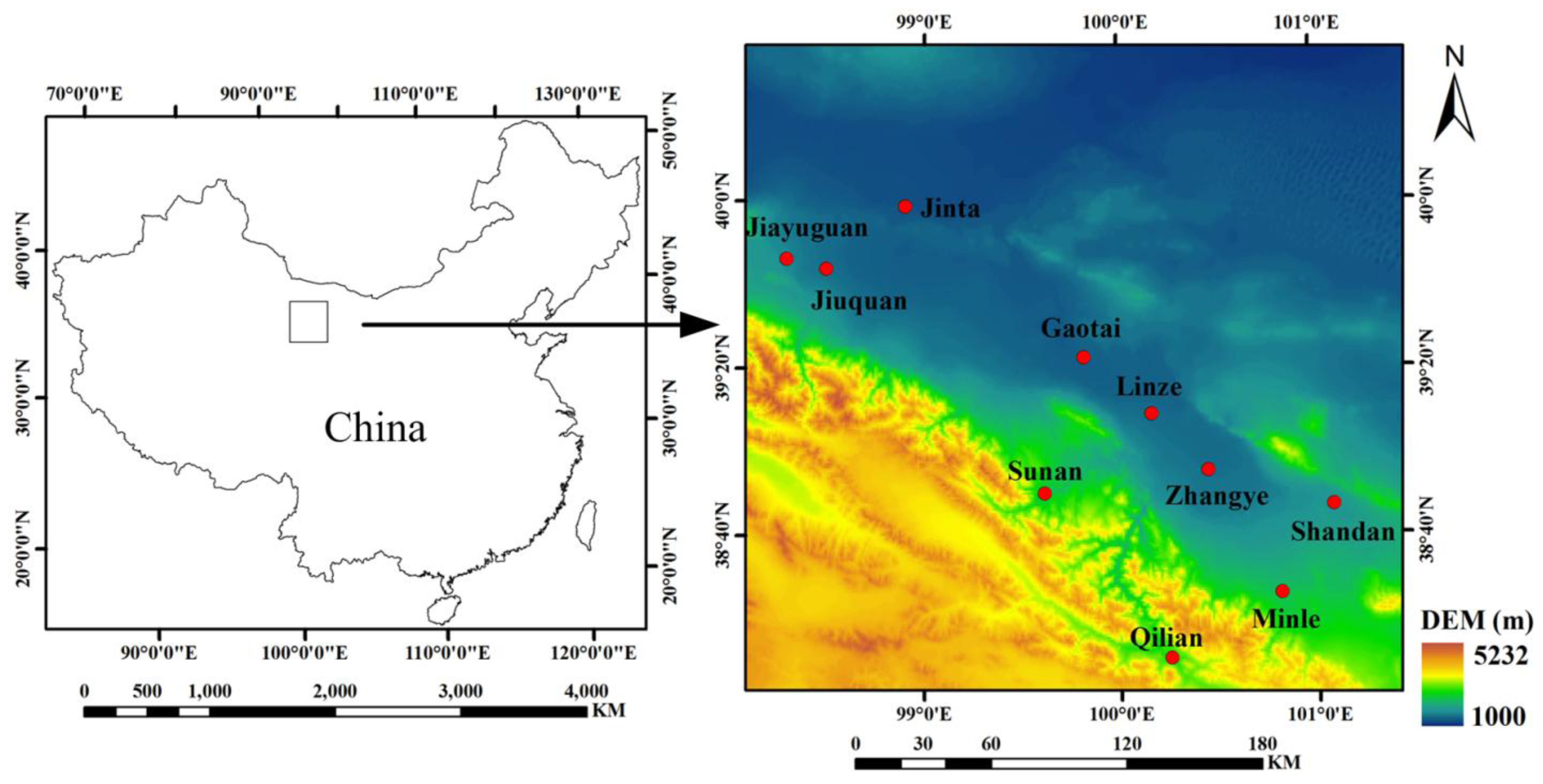
The study area, the Heihe River basin, is located in northwestern China (Figure 1). The Heihe River is the most important inland river in northwestern China. The Heihe River basin has an elevation higher than 1000 m and an arid climate with low atmospheric water vapor content [34]. It is one of the most arid regions in China. The land surface processes in the study area are important components of many field experiments, such as the HEIhe basin Field Experiment (HEIFE) [35]. The Watershed Allied Telemetry Experimental Research (WATER), which was a simultaneous remote sensing and ground-based experiment, was conducted in the study area from March to July of 2008. The overall objectives of this field experiment were to improve the understanding of hydrological and related ecological processes on a catchment scale, to accumulate a comprehensive dataset for the development of watershed science, and to promote the applicability of quantitative remote sensing in watershed science studies [36].

Atmospheric profiles are necessary to investigate the radiative transfer between the Sun-target-sensor paths. Eighteen radiosonde profiles under clear-sky conditions were collected in the study area during the field experiment from March to July of 2008. These radiosonde profiles covered elevations ranging from 1360 m to 3414 m and atmospheric water vapor contents ranging from 0.098 g·cm⁻² to 1.706 g·cm⁻². The March radiosonde profiles represented dry and cold weather, whereas those acquired in July represented relatively humid and warm weather. Outputs of the Global Data Assimilation System (GDAS) were also collected for examining the atmospheric parameters in the study area. GDAS is one of the operational systems of the National Weather Service’s National Center for Environmental Prediction (NCEP). It is run four times per day (at 00, 06, 12, and 18 UTC), and the outputs include geopotential height, atmospheric temperature at 26 fixed pressure levels and relative humidity at 21 levels. The output is in GRIB (GRIdded Binary) format and extends from (0W, 90°S) to (1°W, 90°N), with 1° × 1° spatial resolution. Publications have reported that GDAS outputs yield advantages for applications such as atmospheric correction of thermal infrared remote sensing images [37], at-sensor signal simulation with radiative transfer models [38], and calibration of thermal remote sensors [39]. Four grids located in the study area, including (100°E, 38°N), (100°E, 39°N), (98°E, 40°N), and (99°E, 40°N), were selected to extract the atmospheric profiles. The temporal coverage of the extracted GDAS atmospheric profiles spans January to December 2008. Finally, 422 GDAS atmospheric profiles under clear-sky conditions were extracted to establish the prior knowledge database of the atmospheric state in the study area.

In situ LST measurements were collected near the Biandukou site (location: 100.97°E, 38.27°N; elevation: 2690 m). The land surface at the this site was homogenous during the field experiment, and the dominating land cover type was bare cropland covered by soil and sparse barley straws, as well as some meadows with dry grasses. Simultaneous filed measurements were conducted on 14 March 2008, for comparing the measured LSTs with the LSTs provided by the Terra and Aqua MODIS. Two key areas were selected to collect the ground truths of the LSTs. The locations of these two key areas were (100.98°E, 38.22°N) and (100.97°E, 38.26°N). Both of these two key areas were homogenous with bare soil. The key areas and their surrounding areas were homogenous. The size of each key area was set at 120 by 120 m, and each key area was divided into 16 sub-areas with 30 by 30 m sizes.

During the daytime on 14 March 2008, the overpassing times of the Terra and Aqua satellites were 04:30 and 06:10 (UTC). While the satellites were overpassing, the radiative temperature at the center of each sub-area was measured using Testo handheld infrared thermometers (IRT). The wavelength range of this instrument is 8 μm to 14 μm. The temperature range is −35.0 °C to 950.0 °C, and the precision is ±0.75 °C in the temperature range of −35.0 °C to 75.0 °C. Next, the radiative temperatures within a key area were averaged to denote the radiative temperature of the key area. The measured surface radiative temperatures with IRT were converted to the surface temperatures after correcting the broadband emissivity and atmospheric influences. Due to the lack of instruments for measuring the surface emissivities, the broadband emissivity of bare soil was assumed to be 0.950. Details about the conversion of radiative temperatures to surface temperatures can be found in [40].

2.2. Regression Models for Atmospheric Parameters

The construction of this method involves three stages. In the first stage, the radiative transfer equations of MODIS channels 31 and 32 are simplified. In the second stage, the GDAS atmospheric profiles are used to simulate channel-integrated atmospheric parameters in MODIS channels 31 and 32 based on the MODTRAN4 code [41]. Regression models that describe the relationships between these parameters are developed. In the third stage, new radiative transfer equations are established by substituting the regression models into the simplified radiative transfer equations. The LST is calculated with the genetic algorithm through iteration and optimization processes.

The radiative transfer equation (RTE) in the thermal infrared range is based on the following assumptions [3,42]: (1) the atmosphere is at local thermodynamic equilibrium; (2) no scattering occurs, and thus only cloud-free and non-hazy conditions are considered; and (3) the target is a Lambertian surface. Assuming that the land is a Lambertian surface in the thermal infrared range, the radiative transfer process from the ground to the remote sensor can be described as Equation (1) [43]:

$$L_{\lambda }={\varepsilon }_{\lambda }{\tau }_{\lambda }B(\lambda ,T_{\text{s}})+(1-{\varepsilon }_{\lambda }){\tau }_{\lambda }{L}_{\lambda }^{\downarrow }+L_{\lambda }^{\uparrow }$$

(1)

where λ is the wavelength; L_λ is the TOA radiance; ɛ_λ is the surface emissivity; τ_λ is the total transmittance of the atmosphere; B(λ, T_s) is the radiance emitted by a blackbody at temperature T_s; and $L_{\lambda }^{\downarrow }$ and $L_{\lambda }^{\uparrow }$ are the atmospheric downwelling and upwelling radiance, respectively.

B(λ, T_s) can be calculated using Planck’s function, but deriving an operative expression of the temperature is complex, and the function should be simplified. Applying Taylor’s approximation of radiance around a certain temperature value or linearization is a commonly used method [20,44]. We calculated the channel-integrated radiances of MODIS channels 31 and 32 in the temperature range of 250.0 K to 340.0 K, with a temperature increment of 0.5 K, according to the variability of LST in the study area. Then, the relationships between temperature and radiance in these two thermal channels were investigated. A significant linear relationship was found between the radiance and the temperature. Six linear functions are proposed to replace Planck’s functions of MODIS channels 31 and 32 in three temperature ranges. These linear functions follow the general form:

$$B_i(T)=a_{i}T+b_i$$

(2)

where i = 31, 32; B_i is the radiance in channel i; T is temperature; and a_i and b_i are coefficients. The values a_i, b_i, and the parameters of regression analysis are listed in

Table 2. Coefficients for linearizing Planck’s functions of MODIS channels 31 and 32 in different temperature ranges. The parameters for regression analysis are also shown.

Temperature Range	MODIS Channel	a	b	Adjusted R2	Significance Level	Sample Size
250 K–280 K	31	0.1003	−21.175	0.998	0.001	61
	32	0.0902	−18.637	0.998	0.001	61
280 K–310 K	31	0.1350	−30.917	0.999	0.001	60
	32	0.1169	−26.110	0.999	0.001	60
310 K–340 K	31	0.1693	−41.560	0.999	0.001	60
	32	0.1422	−33.966	0.999	0.001	60

. Equation (2) can also be extended to other areas because the radiance only depends on the temperature and the effective wavelength of the thermal channel.

In Equation (1), the atmospheric upwelling radiance $L_{\lambda }^{\uparrow }$ is usually computed as [45]:

$$L_{\lambda }^{\uparrow }={\int }_0^Z{B}_{\lambda }(T_z)\frac{\partial {\tau }_{\lambda }(\theta ,z,Z)}{\partial z}dz$$

(3)

where Z is the altitude of the remote sensor; T_z is the atmospheric temperature at altitude z; and τ_λ(θ, z, Z) is the upwelling atmospheric transmittance from altitude z to the sensor height Z. After employing the mean value theorem to express the upwelling radiance, $L_{\lambda }^{\uparrow }$ can be expressed as [46]:

$$L_{\lambda }^{\uparrow }=[1-{\tau }_{\lambda }(\theta )]B_{\lambda }(T_{\text{a}})$$

(4)

where T_a is the effective mean atmospheric temperature.

With a similar simplification, $L_{\lambda }^{\downarrow }$ can be calculated as:

$$L_{\lambda }^{\downarrow }=[1-{\tau }_{\lambda }(\theta )]B_{\lambda }(T_{\text{a}}^{\downarrow })$$

(5)

where $T_{\text{a}}^{\downarrow }$ is the average temperature of the atmospheric downwelling radiance. Qin et al. (2001) concluded that using T_a to replace $T_{\text{a}}^{\downarrow }$ in Equation (5) does not have much influence on the accuracy of the retrieved LST [46]. Therefore, it is reasonable to use $L_{\lambda }^{\uparrow }$ replace $L_{\lambda }^{\downarrow }$. Consequently, the channel-integrated thermal radiances acquired by MODIS channels 31 and 32 at TOA can be described as follows:

$$L_i={\varepsilon }_i{\tau }_i{B}_i(T_{\text{s}})+[1+(1-{\varepsilon }_i){\tau }_i]L_i^{\uparrow }$$

(6)

The parameters in Equation (6) have the same meanings as those in Equation (1), and the subscript i means that the parameters are for MODIS channels 31 or 32. According to the correlations between atmospheric radiations in adjacent thermal channels of a sensor, it is reasonable to assume that the atmospheric parameters, including τ₃₁, $L_{31}^{\uparrow }$, τ₃₂, and $L_{32}^{\uparrow }$, can be expressed as functions of a single parameter. Therefore, radiative transfer simulations are conducted to analyze the relationships between these atmospheric parameters. The extracted atmospheric profiles from the described GDAS datasets are put into the MODTRAN4 code to simulate the TOA radiances and other atmospheric parameters. It should be noted that the altitude, pressure, air temperature, and humidity at each layer of each atmospheric profile are used here. The radiative transfer simulations follow these conditions: (1) the MODTRAN4 code is executed in the thermal radiance mode; (2) the sensor view zenith angles in MODTRAN4 are set to range from 0° to 60° in 5° increments to cover the view angles of MODIS; and (3) the sky is clear, and the visibility is 23 km. The water vapor content along the atmospheric path can be extracted from MODTRAN4 outputs. The simulated parameters are converted to the channel-integrated values following [47]:

$$<x>=\frac{{\int }_{{\lambda }_{\text{min}}}^{{\lambda }_{\text{max}}}x(\lambda )f(\lambda )d\lambda }{{\int }_{{\lambda }_{\text{min}}}^{{\lambda }_{\text{max}}}f(\lambda )d\lambda }$$

(7)

where <x> is the channel-integrated value of the parameter x; λ_min and λ_max are the lower and upper wavelengths of the corresponding channels; x(λ) is the value of parameter x at wavelength λ; and f(λ) is the spectral response function.

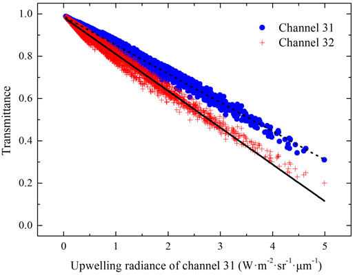
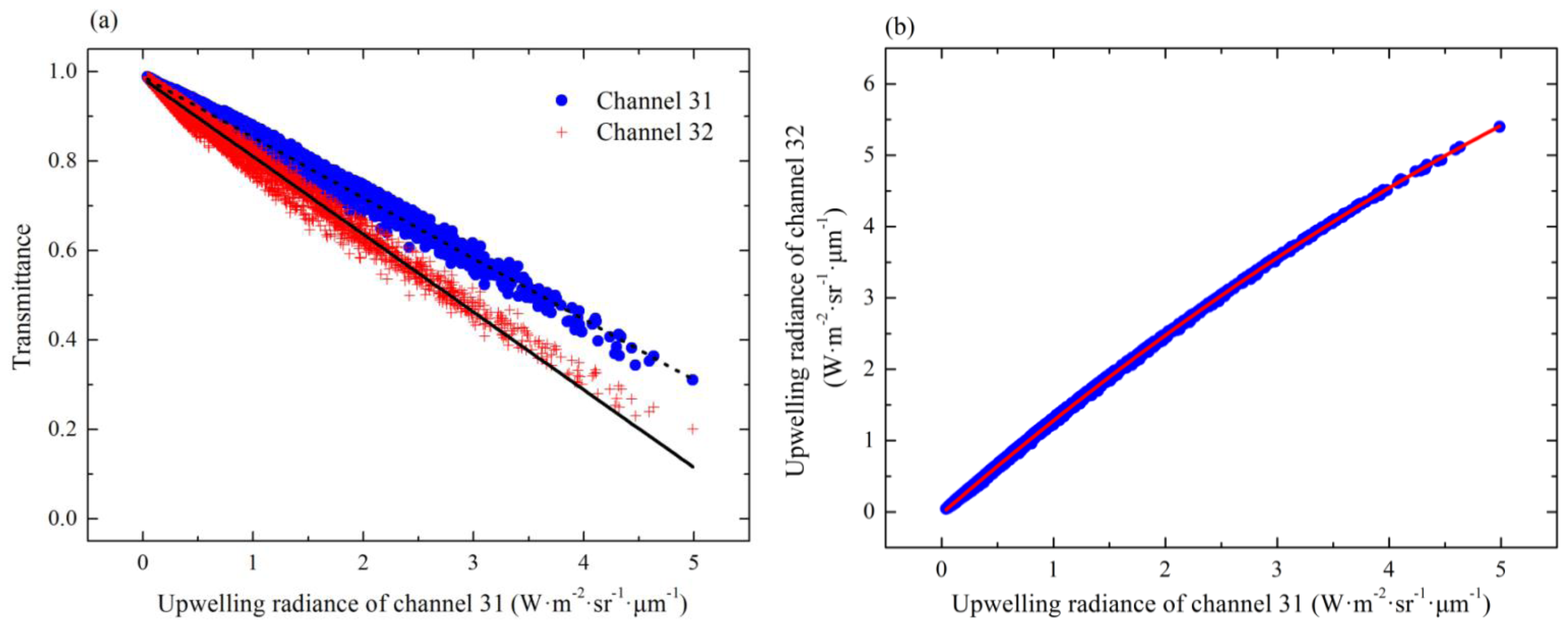
In total, 5486 samples covering 13 zenith angles for all GDAS atmospheric profiles are used to analyze the relationships between τ₃₁, τ₃₂, $L_{31}^{\uparrow }$ and $L_{32}^{\uparrow }$. The scatter plots between $L_{31}^{\uparrow }$ and the other three parameters are displayed in Figure 2. Regression analysis reveals that τ₃₁ and τ₃₂ can be linearly parameterized by $L_{31}^{\uparrow }$ with sufficient accuracy, and $L_{32}^{\uparrow }$ can be estimated by $L_{31}^{\uparrow }$ with a quadric function. The adjusted R² values used to establish the regressions between τ₃₁, τ₃₂, $L_{32}^{\uparrow }$ and $L_{31}^{\uparrow }$ are 0.990, 0.988, and 1.0, respectively. All the correlations are significant at the 0.001 probability level. The formula is listed below:

$$\left[\begin{array}{c}{\tau }_{31}(L_{31}^{\uparrow })\\ {\tau }_{32}(L_{31}^{\uparrow })\\ L_{32}^{\uparrow }(L_{31}^{\uparrow })\end{array}\right]=\left[\begin{array}{ccc}0& -0.136& 0.988\\ 0& -0.174& 0.984\\ -0.054& 1.358& -0.023\end{array}\right]\hspace{0.17em}\left[\begin{array}{c}{L_{31}^{\uparrow }}^2\\ L_{31}^{\uparrow }\\ 1\end{array}\right]$$

(8)

We use the eighteen radiosonde profiles collected during the field experiment to quantify the uncertainties of Equation (8). The simulated $L_{31}^{\uparrow }$ of all the radiosonde profiles based on the MODTRAN4 code are used to calculate τ₃₁, τ₃₂ and $L_{32}^{\uparrow }$ following Equation (8). Statistics on the errors of the calculated values, including the error ranges, standard deviations of the error and absolute error, mean absolute errors (MAEs), and root-mean-square errors (RMSEs), are presented in

Table 3. Statistics on the errors of the calculated τ₃₁, τ₃₂ and $L_{32}^{\uparrow }$ based on $L_{31}^{\uparrow }$ for the radiosonde profiles collected during the field experiment.

Parameter	Error Range	Standard Deviation of the Error	Standard Deviation of the Absolute Error	MAE	RMSE
τ31	−0.0189–0.0042	0.0059	0.0054	0.0080	0.0097
τ32	−0.0221–0.0035	0.0044	0.0042	0.0098	0.0107
$L_{32}^{\uparrow }(\text{W}·{\text{m}}^{-2}·{\text{sr}}^{-1}·\mathrm{\mu }{\text{m}}^{-1})$	−0.0144–0.0517	0.0122	0.0098	0.0083	0.0128

. Based on Table 3, it can be concluded that the regression models are highly accurate. Table 3 also demonstrates that the calculated τ₃₂ has a slightly larger error than τ₃₁ does because MODIS channel 32 suffers stronger significant atmospheric influences than channel 31 does.

2.3. Determination of LST with a Genetic Algorithm

The genetic algorithm (GA) is a technique for searching and optimizing based on selection and natural genetics [48]. The basic principle of the GA is similar to natural selection and inheritance during biological evolution. It begins with a population that contains potential solutions. Then, an objective function is used to assess each potential solution. The solutions with good abilities are selected and inherited by the next generation. The other solutions are changed by mutation or crossover. The new potential solutions are assessed again with the objective function. The iteration process stops when the objective function reaches the defined threshold or the iteration time exceeds a pre-defined value. Compared with other optimization algorithms, the GA has a good ability for global optimization and does not trend to a local solution. The GA has a high probability of finding the global optimal solution even when the objective function has noise [49].

The GA can resolve ill-posed problems where there are more unknowns than equations. These ill-posed problems are common when retrieving parameters from remote sensing data. Xu et al. (2001) and Zhuang et al. (2001) reported instances where the GA was used to retrieve the component temperature from multi-angular thermal remote sensing images, and they concluded that the GA is a robust tool for estimating the component temperature [50,51]. Song and Zhao (2007) applied the GA to retrieve component temperature from MODIS data based on a linear spectral mixing model [52]. The GA appears to be a good method for retrieving the LST from thermal remote sensing images.

In the case where LSEs in MODIS channels 31 and 32 have been obtained, there are two unknowns left after substituting the regression models into the two RTEs. The unknown parameters are LST and $L_{31}^{\uparrow }$. It is straightforward to obtain their analytical solutions. If the LST is calculated directly from the two RTEs, the errors and noises of the parameters (e.g., LSEs) and regression models may lead to an unacceptable error in the LST. To obtain physically meaningful estimations, the variation ranges of LST and $L_{31}^{\uparrow }$ should be determined first to constrain the equation solutions. The GA is able to generate stable results and is not sensitive to the parameter errors or noises with the objective function [49,50]. Furthermore, the GA does not tend to generate local solutions for non-linear inversion problems. Although a disadvantage of using the GA for solving multi-dimensional problems is that it is time-consuming, the present problem that must be solved is positive definite, and the GA is efficient. Therefore, the GA algorithm in the Global Optimization Toolbox provided by the Matlab software is used here.

After replacing τ₃₁, τ₃₂, and $L_{32}^{\uparrow }$ in the RTEs of MODIS channels 31 and 32 with Equation (8), two new RTEs are obtained, as follows:

$$L_{31}={\varepsilon }_{31}{\tau }_{31}(L_{31}^{\uparrow })B_{31}(T_{\text{s}})+[1+(1-{\varepsilon }_{31}){\tau }_{31}(L_{31}^{\uparrow })]L_{31}^{\uparrow }$$

(9)

$$L_{32}={\varepsilon }_{32}{\tau }_{32}(L_{31}^{\uparrow })B_{32}(T_{\text{s}})+[1+(1-{\varepsilon }_{32}){\tau }_{32}(L_{31}^{\uparrow })]L_{32}^{\uparrow }(L_{31}^{\uparrow })$$

(10)

The configuration of GA for calculating LST from Equations (9) and (10) contains the following four steps:

(1)

Defining the ranges of $L_{31}^{\uparrow }$ and T_s: The ranges of $L_{31}^{\uparrow }$ and T_s are defined as 0.01 W·m⁻²·sr⁻¹·μm⁻¹ to 3.0 W·m⁻²·sr⁻¹·μm⁻¹ and 250.0 K to 340.0 K, respectively. The previous two ranges are set according to the conditions of the study area and our investigations of the radiosonde profiles, GDAS profiles, and MODIS LST/emissivity products. On the one hand, the maximum value of $L_{31}^{\uparrow }$ calculated based on all the in situ atmospheric radiosondes is 1.8821 W·m⁻²·sr⁻¹·μm⁻¹, appearing in the region with low elevation in summer. For all the GDAS profiles, over 98% of the simulated samples have $L_{31}^{\uparrow }$ lower than 3.0 W·m⁻²·sr⁻¹·μm⁻¹, and the GDAS profiles are found to overestimate the water vapor contents. On the other hand, a range of 250.0 K to 340.0 K covers most possible conditions in the study area, according to our finding based on MODIS LST products of the study area.

(2)

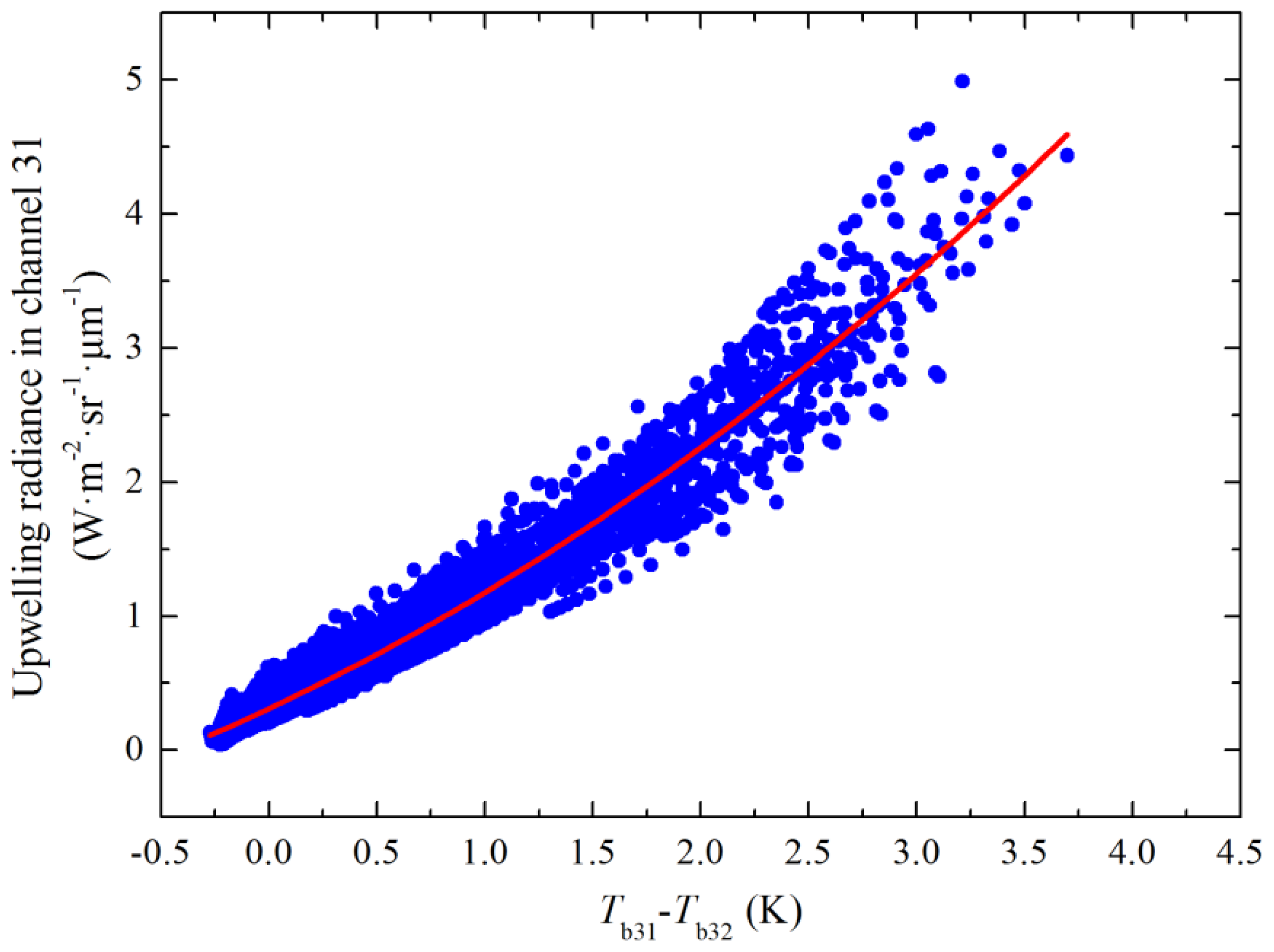
Defining the initial values of T_s and $L_{31}^{\uparrow }$: Considering that the atmospheric effects in MODIS channel 32 are more significant than those in channel 31, the at-sensor brightness temperature of channel 31, T_b31, is used as the initial value of T_s. It is difficult to determine the initial value of $L_{31}^{\uparrow }$ because there is no knowledge about the atmospheric condition. However, we find that there is a significant correlation between $L_{31}^{\uparrow }$ and T_b31–T_b32 (see Figure 3). Their relationship can be written as:

$$L_{31}^{\uparrow }=0.108{(T_{\text{b}31}-T_{\text{b}32})}^2+0.758(T_{\text{b}31}-T_{\text{b}32})+0.310$$

(11)

In total, 5486 samples are used to infer Equation (11). The adjusted R² value of the regression is 0.964, and the correlation is significant at the 0.001 probability level, demonstrating that Equation (11) is sufficiently accurate to calculate the initial value of $L_{31}^{\uparrow }$. Because of the searching and optimizing processes, the results generated by the GA are not significantly influenced by the initial values of the unknowns.

(3)

Designing the objective function of GA: The estimated T_s and $L_{31}^{\uparrow }$ should balance the radiative transfer equations. Therefore, the following function is used as the objective function to select appropriate individuals during iteration:

$$F={\left\{L_{31}-{\varepsilon }_{31}{\tau }_{31}(L_{31}^{\uparrow })B_{31}(T_{\text{s}})-\left[1+(1-{\varepsilon }_{31}){\tau }_{31}(L_{31}^{\uparrow })\right]L_{31}^{\uparrow }\right\}}^2+{\left\{L_{32}-{\varepsilon }_{32}{\tau }_{32}(L_{31}^{\uparrow })B_{32}(T_s)-\left[1+(1-{\varepsilon }_{32}){\tau }_{32}(L_{31}^{\uparrow })\right]L_{32}^{\uparrow }(L_{31}^{\uparrow })\right\}}^2$$

(12)

where the objective value, F, should be close to 0.

(4)

Specifying the population size (Popsize), maximum number of generations (Maxgen), crossover fraction (Pc) and mutation fraction (Pm): These parameters may significantly influence the optimization of GA [50–52]. Determining these parameters is a repetitive process. A group of parameters derived from the simulation of a radiosonde profile, which were acquired at the Biandukou site on 5 July 2008, is used for an experiment. These parameters are an LST of 300.9 K, TOA spectral radiances of 9.3994 W·m⁻²·sr⁻¹·μm⁻¹ and 8.7839 W·m⁻²·sr⁻¹·μm⁻¹ for channels 31 and 32, respectively.

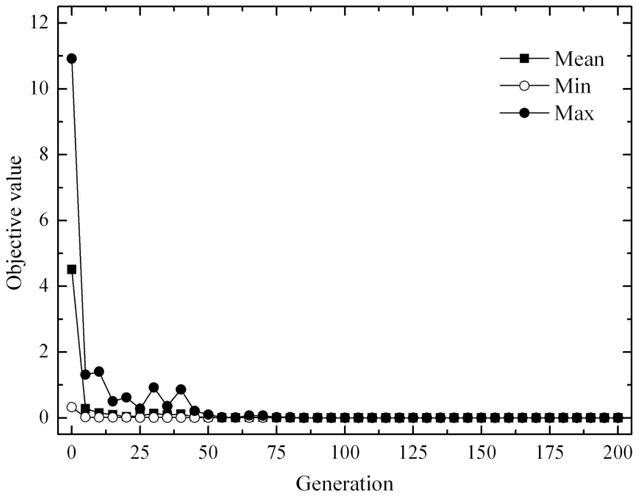
First, Popsize is set to range from 10 to 90, and the Maxgen is set to range from 20 to 180. These two ranges are set by following the trial and error process. The GA is run five times for each Popsize and Maxgen pair, and the MAE of the retrieved LSTs is calculated (

Table 4. MAEs of the retrieved land surface temperatures with different population sizes and maximum generations in the genetic algorithm.

Population Size (Popsize)	Maximum Generation (Maxgen)
	20	60	100	140	180
10	2.7	1.1	0.3	0.7	0.6
30	0.3	0.4	0.5	0.3	0.3
50	0.5	0.5	0.3	0.3	0.3
70	0.4	0.4	0.3	0.3	0.3
90	0.3	0.4	0.3	0.3	0.3

). Figure 4 shows example minimum, mean, and maximum objective values of all individuals in each generation during the iteration process. The LST error decreases when Popsize increases. Setting Maxgen as 100 and Popsize as 50 is a good timesaving choice. The convergence becomes very stable after the maximum number of generations reaches 100.

Second, we examine the determination of the mutation fraction and crossover fraction (Pc) of the GA. The GA uses the mutation and crossover functions to produce new individuals at each generation. In this research, Pm is set as “adaptive feasible” for constrained minimization, which randomly generates adaptive directions with respect to the last successful or unsuccessful generation. Pc is commonly set at 0.4 to 0.9. A smaller value of Pc will limit the ability for an individual to mutate and find the global optimum, but a greater value will cause an unstable solution of the GA [52]. We chose values for Pc ranging from 0.4 to 0.9 with an increment of 0.1 and tested the GA five times for each Pc value. The errors of the calculated LSTs are listed in

Table 5. Errors in the retrieved land surface temperatures with different crossover fractions in the genetic algorithm.

Time	Crossover Fraction (Pc)
	0.4	0.5	0.6	0.7	0.8	0.9
1	0.3	0.3	0.3	0.3	0.3	0.3
2	0.3	0.3	0.3	0.3	0.3	0.4
3	0.3	0.3	0.3	0.3	0.3	0.4
4	0.3	0.3	0.3	0.3	0.3	0.3
5	0.3	0.3	0.3	0.3	0.3	0.5

. Table 5 shows that the LST errors are 0.3 when the Pc is 0.4 to 0.8. The LST error increases when Pc is 0.9. This phenomenon suggests that premature convergence occurs. The GA requires a relatively long time to converge when Pc is set to a smaller value. Pc is set to 0.8 in this research.

3. Sensitivity Analysis and Validations

3.1. Sensitivity Analysis

Sensitivity analysis is important for developing the LST retrieval algorithms. Such analyses have been reported in publications, e.g., Becker and Li (1990) [14], Li and Becker (1993) [53], and Qin et al. (2001) [46]. Here, the sensitivities of the proposed RM-GA method to the errors of LSEs and at-sensor brightness temperatures of MODIS channels 31 and 32 are investigated because errors in these parameters may lead to errors in the LST. The LST error can be calculated as follows:

$$\delta T_{\text{s}}=|T_{\text{s}}(x+\delta x)-T_{\text{s}}(x)|$$

(13)

where δT_s is the error in LST; x is the parameter on which the sensitivity analysis is performed; and δx is the error in x.

Four instances are considered in the sensitivity analysis including LST errors on δɛ₃₁, δɛ₃₂, δT_b31 and δ(T_b31–T_b32). Radiosonde profiles BG0314 and YK0707 are selected and put into the MODTRAN4 code to simulate the at-sensor spectral radiances of MODIS channels 31 and 32. Next, the simulations are used to estimate the LSTs using the RM-GA method. Radiosonde BG0314 was collected at the Biandukou site on 14 March 2008. It represented a cold and arid atmosphere. Radiosonde YK0707 was collected at the Yingke site, located at 100°25′E, 38°51′N and with an elevation of 1486 m, on 7 July 2008. It represented hot and humid weather. For each profile, the sensitivity analysis is conducted at two view zenith angles (i.e., 0° and 30°) for two land cover types (i.e., soil and vegetation). For soil, the LSEs are defined as 0.970 for MODIS channel 31 and channel 32; for vegetation, the LSEs are defined as 0.986 and 0.988 for these two channels. LST is set as the temperature of the bottom atmosphere layer for each profile.

LST errors, which are caused by LSE errors, for the two radiosonde profiles are presented in

Table 6. Land surface temperature (LST) error caused by errors in the LSEs of MODIS channels 31 and 32 for radiosonde profile BG0314.

LSE Error	LST Error Caused by δɛ31				LST Error Caused by δɛ32
	Soil, VZA = 0	Soil, VZA = 30	Vegetation, VZA = 0	Vegetation, VZA = 30	Soil, VZA = 0	Soil, VZA = 30	Vegetation, VZA = 0	Vegetation, VZA = 30
−0.010	1.4	1.3	1.2	1.2	0.8	0.8	0.6	0.6
−0.008	1.1	1.1	0.9	0.9	0.6	0.6	0.5	0.5
−0.006	0.8	0.8	0.7	0.7	0.5	0.5	0.3	0.3
−0.004	0.5	0.5	0.5	0.5	0.3	0.3	0.2	0.2
−0.002	0.3	0.3	0.2	0.2	0.1	0.1	0.1	0.1
0.0	0.0	0.0	0.0	0.0	0.0	0.0	0.0	0.0
0.002	0.3	0.3	0.2	0.2	0.1	0.1	0.1	0.1
0.004	0.5	0.5	0.5	0.5	0.3	0.3	0.2	0.2
0.006	0.8	0.8	0.7	0.7	0.4	0.4	0.3	0.3
0.008	1.1	1.1	0.9	0.9	0.5	0.5	0.4	0.4
0.010	1.4	1.4	1.2	1.2	0.6	0.6	0.5	0.5

and

Table 7. LST error caused by errors in the LSEs of MODIS channels 31 and 32 for radiosonde profile YK0707.

LSE Error	LST Error Caused by δɛ31				LST Error Caused by δɛ32
	Soil, VZA = 0	Soil, VZA = 30	Vegetation, VZA = 0	Vegetation, VZA = 30	Soil, VZA = 0	Soil, VZA = 30	Vegetation, VZA = 0	Vegetation, VZA = 30
−0.010	2.0	1.9	2.1	1.9	1.8	2.0	1.8	2.3
−0.008	1.6	1.5	1.7	1.6	1.7	2.2	1.9	2.4
−0.006	1.3	1.2	1.3	1.2	1.9	2.3	2.0	1.3
−0.004	0.9	0.8	0.9	0.8	0.9	0.7	2.2	0.7
−0.002	0.4	0.4	0.5	0.4	0.4	0.3	0.4	0.3
0.0	0.0	0.0	0.0	0.0	0.0	0.0	0.0	0.0
0.002	0.5	0.4	0.5	0.5	0.3	0.3	0.3	0.3
0.004	1.1	1.1	1.2	1.0	0.6	0.5	0.6	0.6
0.006	2.2	1.6	2.3	1.5	0.8	0.8	0.9	0.8
0.008	2.5	2.7	2.7	2.8	1.1	1.0	1.1	1.0
0.010	2.7	2.9	2.8	3.1	1.3	1.2	1.4	1.2

. Sensitivity analysis reveals that underestimating the emissivity of MODIS channel 31 will cause the overestimation of LST, and vice versa. The sensitivity of LST on δɛ₃₁ varies with atmospheric conditions. For the BG0314 profile, δT_s is up to 1.4 K when δɛ₃₁ is 0.01 and up to 3.2 K when δɛ₃₁ is 0.02. For the YK0707 profile, δT_s is up to 3.1 K and 3.7 K when δɛ₃₁ is 0.01 and 0.02, respectively. The LST sensitivity also slightly depends on the land cover type, but such dependence appears to vary with atmospheric conditions. In addition, the VZA has slight influences on the LST sensitivities.

The channel 32 emissivity has much lower influence on the LST error compared with the channel 31 emissivity. For the BG0314 profile, δT_s is up to 0.8 K and 2.2 K when δɛ₃₂ is up to 0.01 and 0.02, while for the YK0707 profile, δT_s is up to 2.4 K. Therefore, it can be concluded that the LST sensitivities on the LSEs rely on the atmospheric conditions. The proposed RM-GA method is much more sensitive to LSE errors under conditions with humid atmospheres than with dry atmospheres. This fact may be attributed to worse performances of the regression models under such conditions. Fortunately, we find that the varying trends of LST errors caused by emissivities in channels 31 and 32 are opposite. Therefore, the requirement for accurate LSEs in the RM-GA method is reduced.

The sensitivities of the proposed RM-GA method to δT_b31 and δ(T_b31–T_b32) are negligible. δT_s on δT_b31 and δ(T_b31–T_b32) calculated based on Equation (13) are zero. In addition, such sensitivity is independent of the atmospheric condition, land cover type, and VZA.

3.2. Validations

The following three datasets are selected to evaluate the accuracy of the proposed RM-GA method: (1) simulation datasets based on in situ radiosonde profiles and GDAS profiles; (2) in situ measurements of LST in the field experiment; and (3) the daily MODIS LST products. Details can be found in the following sub-sections.

3.2.1. Validation with Simulation Datasets

The simulated at-sensor radiances of MODIS channels 31 and 32 based on the eighteen radiosonde profiles collected in the field experiment are used to retrieve the LST through the proposed RM-GA. A scatter plot relating the estimated LSTs and the input LSTs to the MODTRAN4 code for all radiosonde profiles is displayed in Figure 5. It is evident that most of the samples are close to the 1:1 line. The calculated RMSE and MAE for all the samples are 0.9 K and 0.7 K, respectively. The dependence of the retrieval error on the sensor view zenith angle is weak, thus indicating that the RM-GA method can obtain a similar accuracy at large and small view angles.

In addition, the simulated at-sensor radiances of MODIS channels 31 and 32, based on the GDAS profiles, are placed into the RM-GA method to estimate the LST. The details are shown in

Table 8. Validation of the RM-GA method with simulations of GDAS profiles in the study area.

Grid Location	Sample Size	MAE (K)	RMSE (K)
(100°E, 38°N)	1495	0.8	1.0
(100°E, 39°N)	1339	0.5	0.7
(98°E, 40°N)	1326	0.6	0.8
(99°E, 40°N)	1326	0.6	0.8
Total	5486	0.6	0.9

. The RMSEs of these four grids range from 0.7 K to 1.0 K, and the MAEs range from 0.5 K to 0.8 K. The overall MAE and RMSE for all the profiles are 0.6 K and 0.9 K, respectively.

3.2.2. Validation with In Situ LST Measurements

The in situ measured LSTs described in Section 2.1 are also used to validate the proposed RM-GA method. The measured and retrieved LSTs are listed in

Table 9. Comparisons of the LSTs provided by the in situ measurements, the RM-GA method and the daily MODIS LST/emissivity products.

Satellite	Location	Measured LST (K)	Estimated LST by RM-GA (K)	MODIS product (K)
Terra	100.98°E, 38.22°N	292.2	291.5	290.2
	100.97°E, 38.26°N	291.7	290.3	290.7
Aqua	100.98°E, 38.22°N	294.2	294.0	294.4
	100.97°E, 38.26°N	294.3	293.1	294.1

. The LSTs of the two key areas extracted from the daily MODIS LST/emissivity products (i.e., MOD11A1 and MYD11A1) in version V005 are also shown for comparison purposes. The MAE and RMSE for the LSTs retrieved using our method are 0.9 K and 1.0 K, respectively. The MAE and RMSE for the LSTs provided by the MODIS LST/emissivity products are 0.9 K and 1.1 K, respectively. Comparisons of the two key areas demonstrate that the proposed RM-GA method is accurate for actual MODIS images for the study area.

3.2.3. Comparisons with MODIS LST Products

LSTs retrieved with the RM-GA method are further compared with those extracted from MOD11A1 LST/emissivity products, which yield 1.0 K accuracy for surfaces with known emissivities [54]. The selected MODIS images were acquired by Terra MODIS at 04:05 and 15:10 (UTC) on 6 July 2007. A region covering part of the study area under clear-sky conditions was selected. The images were acquired in the summer, when the atmosphere in the study area is relatively humid and warm. Therefore, it is a typical data source to test our method.

The land surface emissivities of MODIS channels 31 and 32 that are necessary for the proposed method are calculated according to [55]. In general, the spatial patterns of LSTs derived from the RM-GA method and MODIS LST products are similar (Figure 6): the gobis and deserts exhibited high surface temperatures, vegetation such as croplands and meadows yielded moderate temperatures, and the partly snow-covered mountains in the southern part of the region were the coldest. The temperature ranges for the entire region derived from both methods are similar. For our method, the LST ranges were 270.5 K to 330.0 K and 262.2 K to 297.2 K at 04:05 and 15:10, respectively. The LST ranges derived from MODIS LST products were 271.2 K to 330.9 K and 262.3 K to 296.0 K, respectively. Comparisons reveal that 89.7% of all the pixels had a −1.0 K to 2.0 K deviation from the MODIS LST/emissivity product for the daytime image, whereas 91.5% of all the pixels yielded a −1.0 K to 3.0 K deviation from the MODIS product for the nighttime image.

The LST estimations based on the RM-GA method were slightly higher than those provided by the MODIS products for many pixels. The positive deviation of the LSTs estimated by our method from those provided by the MODIS products might result from the replacement of the atmospheric downwelling radiances with the atmospheric upwelling radiances in the RTEs because the atmospheric downwelling radiance in MODIS channel 31 or channel 32 is higher than the atmospheric upwelling radiance in the corresponding channel.

4. Discussion

Developing split-window (SW) algorithms for estimating LSTs from thermal sensors with two or more channels in the range of 10–12 μm has been a hot topic in the remote sensing domain over the past several decades. Some of these SW algorithms can provide accurate and stable LSTs, such as the generalized SW algorithm for generating the MODIS LST/emissivity products [15]. In addition to the LSE, many SW algorithms rely on other auxiliary parameters, e.g., the atmospheric water vapor content. The similarities of spectral responses of the thermal channels stimulate us to attempt to reduce the unknowns when solving the radiative transfer equations.

Although there have been numerous algorithms proposed by literatures for deriving LSTs from MODIS data, MODIS is still selected as a test case to develop the RM-GA method because MODIS has excellent calibration accuracy, friendly preprocessing tools and recognized land surface products. Its LST/emissivity product is beneficial for validating the RM-GA method. However, the proposed method is not limited to MODIS and can easily be extended to other satellite thermal sensors with similar channels as MODIS channels 31 and 32. For example, the spectral range of AVHRR channels 4 and 5 are approximately 10.0 to 11.5 μm and 11.5 to 12.5 μm, respectively. The ASTER sensor on board Terra satellite has two similar channels in the previous spectral range, i.e., channel 13 from 10.25 to 10.95 μm and channel 14 from 10.95 to 11.65 μm. These two channels have been proven reliable for estimating LSTs with the split-window algorithm [56]. In addition, the Thermal Infrared Sensor (TIRS) carried by the Landsat-8 satellite (launched as the Landsat Data Continuity Mission—LDCM- on 11 February 2013) also obtains two similar channels. The wavelengths of the first and second channels are 10.6 μm to 11.19 μm and 11.5 μm to 12.51 μm, respectively. With the simulation dataset generated based on GDAS atmospheric profiles in the study area, we find that the regression models for the previously mentioned sensors have the following general form:

$$\left[\begin{array}{c}{\tau }_1(L_1^{\uparrow })\\ {\tau }_2(L_1^{\uparrow })\\ L_2^{\uparrow }(L_1^{\uparrow })\end{array}\right]=\left[\begin{array}{ccc}{a}_{11}& a_{12}& a_{13}\\ a_{21}& a_{22}& a_{23}\\ a_{31}& a_{32}& a_{33}\end{array}\right]\hspace{0.17em}\left[\begin{array}{c}{L_1^{\uparrow }}^2\\ L_1^{\uparrow }\\ 1\end{array}\right]$$

(14)

where a_ij is the coefficient (i = 1, 2, and 3; j = 1, 2, and 3); the subscripts 1 and 2 denote the first and second channels described previously. The coefficients are listed in

Table 10. Coefficient in Equation (14) for AVHRR, ASTER, and TIRS sensors derived from the simulation dataset generated based on GDAS atmospheric profiles.

Satellite and Sensor	ai1 (i = 1, 2, 3)	ai2 (i = 1, 2, 3)	ai3 (i = 1, 2, 3)	Adjusted R2	Standard Error of Estimate
NOAA-7 AVHRR	0	−0.134	0.987	0.989	0.0097
	0	−0.181	0.981	0.986	0.0150
	−0.073	1.460	−0.035	0.999	0.0290
NOAA-9 AVHRR	0	−0.134	0.987	0.989	0.0096
	0	−0.178	0.985	0.986	0.0147
	−0.060	1.411	−0.046	0.999	0.0330
NOAA-11 AVHRR	0	−0.134	0.987	0.989	0.0097
	0	−0.180	0.983	0.986	0.0150
	−0.067	1.436	−0.039	0.999	0.0302
NOAA-12 AVHRR	0	−0.135	0.987	0.989	0.0098
	0	−0.181	0.976	0.986	0.0150
	−0.081	1.482	−0.019	0.999	0.0240
NOAA-14 AVHRR	0	−0.134	0.987	0.989	0.0097
	0	−0.186	0.976	0.985	0.0160
	−0.088	1.531	−0.025	0.999	0.0298
Terra ASTER	0	−0.133	0.986	0.989	0.0095
	0	−0.156	0.996	0.984	0.0132
	0	1.132	−0.053	0.997	0.0397
Landsat-8 TIRS	0	−0.135	0.984	0.988	0.0105
	0	−0.175	0.991	0.987	0.0143
	−0.030	1.299	−0.071	0.999	0.0309

.

In this research, the RM-GA method is proposed for local application in the Heihe River basin, which has an arid climate with low atmospheric water vapor content. The atmospheric effects in the study area are weaker than those in humid regions. The correlations between atmospheric parameters decrease when the atmospheric water vapor content increases [25]. Our research confirms this finding. Accuracies of the regression models decrease when the atmospheric upwelling radiance increases. This phenomenon may increase the error of the retrieved LST. Thus, the applicability of the proposed method to regions with a humid atmosphere is limited. However, it is feasible to extend the proposed method to regions with arid climates and high elevations, e.g., the Qinghai-Tibet Plateau, the Sahara Desert and the Middle East. It is critical that these regions are ecologically vulnerable, and they require satellite LSTs in monitoring the climate changes and in other applications.

In addition to the LST, the RM-GA method provides a possible way to estimate the atmospheric upwelling radiance from the thermal infrared data. To our knowledge, the atmospheric upwelling radiance is an important parameter in atmospheric corrections. Therefore, the RM-GA method may benefit the removal of atmospheric path radiance from thermal data. This preprocessing is required by some other methods, such as the TES algorithms.

The development of the RM-GA method is based on some important assumptions or simplifications. The first is that the land is a Lambertian surface. Therefore, a commonly used simplified radiative transfer equation is used. In fact, many land surfaces are far from Lambertian bodies, and their emission and reflection varies with the zenith and azimuth viewing angles. This thermal anisotropy effect is another key question related to thermal remote sensing. Detailed models are still necessary to examine and model the thermal anisotropy effect thoroughly. Another simplification is that the aerosol condition of the study area has been assumed stable when conducting the radiative transfer simulations. In fact, the aerosol influences the atmospheric transmittance [57]. A larger simulation dataset containing different aerosol conditions might be better than the current one used in this research.

The accuracies of LSEs have great effects on the performance of the RM-GA method, as proven in the sensitivity analysis. Therefore, the RM-GA method relies on accurate determinations of LSEs. Determinations of LSEs in the thermal channels can be conducted with the commonly used Normalized Difference Vegetation Index Thresholds Method (NDVI^THM) or Classification-based Emissivity Method (CBEM) with good accuracies, e.g., approximately 0.02 for the former method [58]. However, the emissivities of bare soil are still difficult to determine. Fortunately, we found that the errors of emissivities in MODIS channels 31 and 32 have opposite impacts on the LST errors. Therefore, the rigorous requirement for accurate emissivities in the RM-GA method may be partially mitigated.

Validation of the LST retrieval methods is an important step for developing algorithms and guarantees the application of such methods. However, such validation is a difficult task and is influenced by many factors. In our previous research on validating the Landsat-5 TM LSTs with surface measurements, we found that deviations of the retrieved LSTs from the measured values might be attributed to the following sources [59]: errors in the in situ measurement of the LST, the measurement accuracy of the instruments and errors caused by their calibrations, the scale mismatch between pixels on the remote sensing image and the sampled LSTs, errors in the retrieved results due to a lack of in situ measured land surface emissivities, and the calibration of satellite sensors. Further comprehensive validations are still required to quantify the accuracies of the estimated LSTs based on remote sensing.

5. Conclusions

Many split-window (SW) algorithms require auxiliary atmospheric parameters (e.g., water vapor content) to calculate land surface temperatures (LSTs) from satellite sensors with two adjacent thermal channels located in the atmospheric window between 10 μm and 12 μm. In this research, the Heihe River basin, which is one of the most arid regions in China and consistently has low atmospheric water vapor content, was selected as the study area. For the study area, we found that correlations between the atmospheric parameters of two adjacent channels provide the possibility to reduce the unknowns when calculating the LST by solving the radiative transfer equations.

MODIS was selected as a test case to develop a so-called regression model—genetic algorithm (RM-GA)-based method because MODIS has excellent calibration accuracy, friendly preprocessing tools, and recognized land surface products. To develop the RM-GA method, the Global Data Assimilation System (GDAS) atmospheric profiles of the study area were used to generate the training dataset through radiative transfer simulation. The relationships between the atmospheric upwelling radiance in MODIS channel 31 and the other three atmospheric parameters, including the transmittance in channel 31 and the transmittance and upwelling radiance in channel 32, were trained based on the simulation dataset and formulated with three regression models. The genetic algorithm was used to estimate the LST.

Validation of the RM-GA method included three aspects. First, validation was performed through the simulations of in situ radiosonde profiles and GDAS atmospheric profiles based on MODTRAN4 code. The accuracy of our method was better than 1.0 K when there was no LSE error. Second, the in situ LSTs measured in the study area were used to assess the proposed method. We found that its accuracy was close to that of the daily MODIS LST/emissivity (MOD11A1) products. Third, a pair of daytime and nighttime MOD11A1 products covering the study area in summer was used as a reference to evaluate the LSTs estimated through the RM-GA method. The comparisons further confirmed that the proposed method is able to provide acceptable estimations of LSTs from MODIS data in the study area. Although this research is for local application in the Heihe River basin, the findings and proposed method can easily be extended to other satellite sensors and regions with arid climates and high elevations.

References

1. Li, Z.L.; Tang, B.H.; Wu, H.; Ren, H.; Yan, G.; Wan, Z.; Trigo, I.F.; Sobrino, J.A. Satellite-derived land surface temperature: Current status and perspectives. Remote Sens. Environ 2013, 131, 14–37. [Google Scholar]
2. Zhou, J.; Chen, Y.H.; Wang, J.F.; Zhan, W.F. Maximum nighttime Urban Heat Island (UHI) intensity simulation by integrating remotely sensed data and meteorological observations. IEEE J. Sel. Topics Appl. Earth Observ 2011, 4, 138–146. [Google Scholar]
3. Qin, Z.H.; Karnieli, A. Progress in the remote sensing of land surface temperature and ground emissivity using NOAA-AVHRR data. Int. J. Remote Sens 1999, 20, 2367–2393. [Google Scholar]
4. Prata, A.J. Land surface temperatures derived from the advanced very high resolution radiometer and the along-track scanning radiometer: 1. Theory. J. Geophys. Res 1993, 98, 16689–16702. [Google Scholar]
5. Snyder, W.C.; Wan, Z.; Zhang, Y.; Feng, Y.Z. Classification-based emissivity for land surface temperature measurement from space. Int. J. Remote Sens 1998, 19, 2753–2774. [Google Scholar]
6. Kealy, P.S.; Hook, S.J. Separating temperature and emissivity in thermal infrared multispectral scanner data: Implications for recovering land surface temperatures. IEEE Trans. Geosci. Remote Sens 1993, 31, 1155–1164. [Google Scholar]
7. Gillespie, A.; Rokugawa, S.; Matsunaga, T.; Cothern, J.S.; Hook, S.; Kahle, A.B. A temperature and emissivity separation algorithm for Advanced Spaceborne Thermal Emission and Reflection Radiometer (ASTER) images. IEEE Trans. Geosci. Remote Sens 1998, 36, 1113–1126. [Google Scholar]
8. Liang, S.L. An optimization algorithm for separating land surface temperature and emissivity from multispectral thermal infrared imagery. IEEE Trans. Geosci. Remote Sens 2001, 39, 264–274. [Google Scholar]
9. Valor, E.; Caselles, V. Mapping land surface emissivity from NDVI: Application to European, African, and South American areas. Remote Sens. Environ 2001, 57, 167–184. [Google Scholar]
10. Ottlé, C.; Vidal-Madjar, D. Estimation of land surface temperature with NOAA-9 data. Remote Sens. Environ 1992, 40, 27–41. [Google Scholar]
11. François, C.; Ottlé, C. Atmospheric corrections in the thermal infrared: Global and water vapor dependent split-window algorithms-Applications to ATSR and AVHRR data. IEEE Trans. Geosci. Remote Sens 1996, 34, 457–470. [Google Scholar]
12. Price, J.C. Land surface temperature measurements from the split window channels of the NOAA7 advanced very high resolution radiometer. J. Geophys. Res 1984, 89, 7231–7237. [Google Scholar]
13. Ulivieri, C.; Cannizzaro, G. Land surface temperature retrievals from satellite measurements. Acta Astronaut 1985, 12, 977–985. [Google Scholar]
14. Becker, F.; Li, Z. Towards a local split window method over land surfaces. Int. J. Remote Sens 1990, 11, 369–393. [Google Scholar]
15. Wan, Z.; Dozier, J. A generalized split-window algorithm for retrieving land-surface temperature from space. IEEE Trans. Geosci. Remote Sens 1996, 34, 892–905. [Google Scholar]
16. Prata, A.J.; Platt, C.M.R. Land Surface Temperature Measurements from the AVHRR. Proceedings of the 5th AVHRR Data Users Conference, Tromso, Norway, 25–28 June 1991; pp. 433–438.
17. Vidal, A. Atmospheric and emissivity correction of land surface temperature measured from satellite using ground measurements or satellite data. Int. J. Remote Sens 1991, 12, 2449–2460. [Google Scholar]
18. Ulivieri, C.; Castronuovo, M.M.; Francioni, R.; Cardillo, A. A split window algorithm for estimating land surface temperature from satellites. Adv. Space Res 1994, 14, 59–65. [Google Scholar]
19. Sobrino, J.A.; Coll, C.; Casselles, V. Atmospheric corrections for land surface temperature using AVHRR channels 4 and 5. Remote Sens. Environ 1991, 38, 19–34. [Google Scholar]
20. Coll, C.; Caselles, V.; Sobrino, J.A.; Valor, E. On the atmospheric dependence of the split-window equation for land surface temperature. Int. J. Remote Sens 1994, 15, 105–122. [Google Scholar]
21. Sobrino, J.A.; Raissouni, N. Toward remote sensing methods for land cover dynamic monitoring: Application to Morocco. Int. J. Remote Sens 2000, 21, 353–366. [Google Scholar]
22. Ma, Y. Remote sensing parameterization of regional net radiation over heterogeneous land surface of Tibetan Plateau and arid area. Int. J. Remote Sens 2003, 24, 3137–3148. [Google Scholar]
23. Becker, F.; Li, Z. Surface temperature and emissivity at various scales: Definition, measurement and related problems. Remote Sens. Rev 1995, 12, 225–253. [Google Scholar]
24. Jiménez-Muñoz, J.C.; Sobrino, J.A. A generalized single-channel method for retrieving land surface temperature from remote sensing data. J. Geophys. Res 2003, 108. [Google Scholar] [CrossRef]
25. Jiménez-Muñoz, J.C.; Cristóbal, J.; Sobrino, J.A.; Soria, G. Revision of the single-channel algorithm for land surface temperature retrieval from Landsat thermal-infrared data. IEEE Trans. Geosci. Remote Sens 2009, 47, 339–349. [Google Scholar]
26. Chrysoulakis, N.; Cartalis, C. Improving the estimation of land surface temperature for the region of Greece: Adjustment of a split window algorithm to account for the distribution of precipitable water. Int. J. Remote Sens 2002, 23, 871–880. [Google Scholar]
27. Zhao, S.; Qin, Q.; Yang, Y.; Xiong, Y.; Qiu, G. Comparison of two split-window methods for retrieving land surface temperature from MODIS data. J. Earth Syst. Sci 2009, 118, 345–353. [Google Scholar]
28. Yang, J.M.; Qiu, J.H. The empirical expressions of the relation between precipitable water and ground water vapor pressure for some areas in China. Sci. Atmos. Sin 1996, 20, 620–626. [Google Scholar]
29. Yang, J.M.; Qiu, J.H. A method for estimating precipitable water and effective water vapor content from ground humidity parameters. Chin. J. Atmos. Sci 2002, 26, 9–22. [Google Scholar]
30. Li, Z.H.; Muller, J.P.; Cross, P. Comparison of precipitable water vapor derived from radiosonde, GPS, and moderate-resolution imaging spectroradiometer measurements. J. Geophys. Res 2003, 108. [Google Scholar] [CrossRef]
31. Jedlovec, G.J. Precipitable water estimation from high-resolution split window radiance measurements. J. Appl. Meteorol 1990, 29, 863–877. [Google Scholar]
32. Kaufman, Y.J.; Gao, B.C. Remote sensing of water vapor in the near IR from EOS/MODIS. IEEE Trans. Geosci. Remote Sens 1992, 30, 871–884. [Google Scholar]
33. Moriyama, M.; Mima, K.; Arai, K. Comparison of the sea surface temperature estimation methods. Adv. Space Res 1995, 16, 123–126. [Google Scholar]
34. Wang, K.L.; Cheng, G.D.; Jiang, H.; Zhang, L.J. Atmospheric hydrologic cycle over the Qilian-Heihe valley. Adv. Water Sci 2003, 14, 91–97. [Google Scholar]
35. Hu, Y.Q. Research advance about the energy budget and transportation of water vapor in the HEIFE area. Adv. Earch Sci 1994, 9, 30–34. [Google Scholar]
36. Li, X.; Li, X.W.; Li, Z.Y.; Ma, M.G.; Wang, J.; Xiao, Q.; Liu, Q.; Che, T.; Chen, E.X.; Yan, G.J.; et al. Watershed Allied Telemetry Experimental Research. J. Geophys. Res 2008, 114. [Google Scholar] [CrossRef]
37. Tonooka, H. An atmospheric correction algorithm for thermal infrared multispectral data over land-a water-vapor scaling method. IEEE Trans. Geosci. Remote Sens 2001, 39, 682–692. [Google Scholar]
38. Dash, P.; Ignatov, A. Validation of clear-sky radiances over oceans simulated with MODTRAN4.2 and global NCEP GDAS fields against nighttime NOAA15-18 and MetOp-A AVHRR data. Remote Sens. Environ 2008, 112, 3012–3029. [Google Scholar]
39. Hook, S.J.; Vaughan, R.G.; Tonooka, H.; Schladow, S.G. Absolute radiometric in-flight validation of mid infrared and thermal infrared data from ASTER and MODIS on the Terra spacecraft using the Lake Tahoe, CA/NV, USA, automated validation site. IEEE Trans. Geosci. Remote Sens 2007, 45, 1798–1807. [Google Scholar]
40. Huang, M.; Liu, S.; Liu, S.; Zhu, Q. A study of the difference between true surface temperature and radiometric surface temperature. Adv. Earth Sci 2005, 20, 1075–1082. [Google Scholar]
41. Berk, A.; Bernstein, L.S.; Anderson, G.P.; Acharya, P.K.; Robertson, D.C. MODTRAN cloud and multiple scattering upgrades wit application to AVIRIS. Remote Sens. Environ 1998, 65, 367–375. [Google Scholar]
42. Dash, P.; Göttsche, F.M.; Olesen, F.S.; Fisch, H. Land surface temperature and emissivity estimation from passive sensor data: Theory and practice-current trends. Int. J. Remote Sens 2002, 23, 2563–2594. [Google Scholar]
43. Ottlé, C.; Stoll, M. Effect of atmospheric absorption and surface emissivity on the determination of land surface temperature from infrared satellite data. Int. J. Remote Sens 1993, 14, 2025–2037. [Google Scholar]
44. Zhou, J.; Chen, Y.; Zhang, X.; Zhan, W. Modeling the diurnal variations of urban heat islands with multi-source satellite data. Int. J. Remote Sens 2013, 34, 7568–7588. [Google Scholar]
45. França, G.B.; Cracknell, A.P. Retrieval of land and sea surface temperature using NOAA-11 AVHRR data in northeastern Brazil. Int. J. Remote Sens 1994, 15, 1695–1712. [Google Scholar]
46. Qin, Z.H.; Olmo, G.D.; Karnieli, A.; Berliner, P. Derivation of split window algorithm and its sensitivity analysis for retrieving land surface temperature from NOAA-advanced very high resolution radiometer data. J. Geophys. Res 2001, 106, 22655–22670. [Google Scholar]
47. Liang, S.L. Quantitative Remote Sensing of Land Surfaces; John Wiley & Sons: Hoboken, NJ, USA, 2004. [Google Scholar]
48. Van Coillie, F.M.B.; Verbeke, L.P.C.; de Wulf, R.R. Feature selection by genetic algorithms in object-based classification of IKONOS imagery for forest mapping in Flanders, Belgium. Remote Sens. Environ 2007, 110, 476–487. [Google Scholar]
49. Lei, Y.J.; Zhang, S.W.; Li, J.W.; Zhou, C.M. Matlab Toolbox for Genetic Algorithm and Its Application; Xidian University Press: Xi’an, China, 2005. [Google Scholar]
50. Xu, X.R.; Chen, L.F.; Zhuang, J.L. Genetic inverse algorithm for retrieval of component temperature of mixed pixel by multi-angle thermal infrared remote sensing data. Sci. China Ser. D 2001, 44, 363–372. [Google Scholar]
51. Zhuang, J.L.; Chen, L.F.; Xu, X.R. Retrieval of component temperature of continuous vegetation using genetic algorithm. J. Remote Sens 2001, 5, 1–7. [Google Scholar]
52. Song, X.N.; Zhao, Y.S. Study on component temperatures inversion using satellite remotely sensed data. Int. J. Remote Sens 2007, 28, 2567–2579. [Google Scholar]
53. Li, Z.; Becker, F. Feasibility of land surface temperature and emissivity determination from AVHRR data. Remote Sens. Environ 1993, 43, 67–85. [Google Scholar]
54. Wan, Z. New refinements and validation of the MODIS land-surface temperature/emissivity products. Remote Sens. Environ 2008, 112, 59–74. [Google Scholar]
55. Momeni, M.; Saradjian, M.R. Evaluating NDVI-based emissivities of MODIS bands 31 and 32 using emissivities derived by Day/Night LST algorithm. Remote Sens. Environ 2007, 106, 190–198. [Google Scholar]
56. Pu, R.; Gong, P.; Michishita, R.; Sasagawa, T. Assessment of multi-resolution and multi-sensor data for urban surface temperature retrieval. Remote Sens. Environ 2006, 104, 211–225. [Google Scholar]
57. Jiménez-Muñoz, J.C.; Sobrino, J.A. Error sources on the land surface temperature retrieved from thermal infrared single channel remote sensing data. Int. J. Remote Sens 2006, 27, 999–1014. [Google Scholar]
58. Sobrino, J.A.; Raissouni, N.; Li, Z. A comparative study of land surface emissivity retrieval from NOAA data. Remote Sens. Environ 2001, 75, 256–266. [Google Scholar]
59. Zhou, J.; Li, J.; Zhang, L.; Hu, D.; Zhan, W. Intercomparison of methods for estimating land surface temperature from a Landsat-5 TM image in an arid region with low water vapour in the atmosphere. Int. J. Remote Sens 2012, 33, 2582–2602. [Google Scholar]
Figure 1. Location of the study area in mainland China.
Remotesensing 06 05344f1
Figure 2. Scatter plots between the atmospheric upwelling radiance of MODIS channel 31 and the other atmospheric parameters. (a) transmittances of channels 31 and 32; (b) upwelling radiance of channel 32.
Remotesensing 06 05344f2
Figure 3. Scatter plot between the simulated atmospheric upwelling radiance in MODIS channel 31 and differences in the at-sensor brightness temperatures of channel 31 and 32 (Tb31Tb32).
Remotesensing 06 05344f3
Figure 4. The minimum (Min), mean (Mean), and maximum (Max) objective values of all the individuals in each generation during the iteration process.
Remotesensing 06 05344f4
Figure 5. Scatter plot between the estimated LST and the LST input to the MODTRAN4 code for the eighteen radiosonde profiles. The solid line corresponds to a 1:1 relation.
Remotesensing 06 05344f5
Figure 6. Spatial patterns of the land surface temperature in the study area retrieved by the RM-GA method and those provided by MODIS LST/emissivity products. A is vegetation, B is snow, C is gobi, and D is desert. The MODIS images were acquired on 6 July 2007. (a) LST at 04:05UTC retrieved with the RM-GA method. (b) LST at 04:05UTC provided by the MODIS LST/emissivity product. (c) LST at 15:10UTC retrieved with the RM-GA method. (d) LST at 15:10UTC provided by the MODIS LST/emissivity product.
Remotesensing 06 05344f6