Statistical Modeling of Sea Ice Concentration Using Satellite Imagery and Climate Reanalysis Data in the Barents and Kara Seas, 1979–2012

Abstract

Extensive sea ice over Arctic regions is largely involved in heat, moisture, and momentum exchanges between the atmosphere and ocean. Some previous studies have been conducted to develop statistical models for the status of Arctic sea ice and showed considerable possibilities to explain the impacts of climate changes on the sea ice extent. However, the statistical models require improvements to achieve better predictions by incorporating techniques that can deal with temporal variation of the relationships between sea ice concentration and climate factors. In this paper, we describe the statistical approaches by ordinary least squares (OLS) regression and a time-series method for modeling sea ice concentration using satellite imagery and climate reanalysis data for the Barents and Kara Seas during 1979–2012. The OLS regression model could summarize the overall climatological characteristics in the relationships between sea ice concentration and climate variables. We also introduced autoregressive integrated moving average (ARIMA) models because the sea ice concentration is such a long-range dataset that the relationships may not be explained by a single equation of the OLS regression. Temporally varying relationships between sea ice concentration and the climate factors such as skin temperature, sea surface temperature, total column liquid water, total column water vapor, instantaneous moisture flux, and low cloud cover were modeled by the ARIMA method, which considerably improved the prediction accuracies. Our method may also be worth consideration when forecasting future sea ice concentration by using the climate data provided by general circulation models (GCM).

1. Introduction

Sea ice is an important component of the climate system. Sea ice cover can change the surface albedo, which in turn acts to reinforce the initial alteration in ice area [1–3]. Extensive sea ice over Arctic regions is largely involved in heat, moisture, and momentum exchanges between the atmosphere and ocean [4]. This is because the sea ice surface reflects significantly more of the incident solar radiation than open water and because melted water has a significant influence on oceanic circulation [5,6]. Therefore, changes in the extent of sea ice have great potential to influence variations in regional and global climatic systems [7,8].

Although a long-range dataset over a large-scale area is necessary to achieve reliable spatiotemporal analysis, it is difficult to scrutinize sea ice changes due to the lack of in-situ observations [9]. However, Arctic sea ice concentration, extent, and area have been continuously monitored for approximately 34 years. Monitoring has been ongoing since 1979 with the help of satellite-based multichannel passive microwave imaging systems [10] such as Scanning Multichannel Microwave Radiometer (SMMR), Special Sensor Microwave/Imager (SSM/I), and Advanced Microwave Scanning Radiometer (AMSR). Sea ice concentration is defined as the fraction of ice-covered areas at a given point in the ocean. Sea ice extent denotes the sum of ice-covered areas with concentrations of at least 15%, while sea ice area is the product of the ice concentration and each pixel area within the ice extent [11,12]. Recent satellite remote sensing studies show that there has been a significant decline in Arctic sea ice extent [13,14] with the possibility that global warming is occurring more rapidly than before. Therefore, reliable outlooks for sea ice conditions are crucial in understanding the future Arctic environment and global climate change [15].

In the Intergovernmental Panel on Climate Change (IPCC) 4th Assessment Report, six climate models indicated that the Arctic might have sea ice-free summers in the 2030s [16,17]. However, significant differences were found among the results predicted by several climate models evaluating changes in Arctic sea ice cover [16,17]. Consequently, the mechanism behind the recent rapid decrease in sea ice extent, which is not yet fully understood, may result in some uncertainties in the process-based Arctic sea ice module of climate models [18,19]. Some other studies on sea ice changes have employed statistical models based on empirical relationships between sea ice conditions and several explanatory variables e.g., [18,20–26]. Variables in the statistical models include prior information on sea ice, as well as oceanic and atmospheric conditions that can influence sea ice changes. Temperature is reasonably expected to be a major predictor for the current loss of sea ice caused by the atmospheric warming trend over the Arctic area [27,28]. However, statistical predictions require additional climatic variables for a more stable explanation for Arctic sea ice changes [18,29,30]. Such empirical knowledge can help identify the physical processes underlying Arctic sea ice changes [16,31] and can contribute to making reasonable outlooks even without the need for explicit physical mechanisms and realistic initial conditions [29].

Some previous studies have been conducted to develop statistical models for the status of Arctic sea ice at seasonal to annual scales and showed considerable possibilities to explain the impacts of climate changes on Arctic sea ice extent. Drobot and Maslanik [20] exploited a statistical model with four regressors (winter multiyear ice concentration, spring total ice concentration, North Atlantic Oscillation index, and East Atlantic index) in order to explain summer ice conditions in the Beaufort Sea. Drobot [21] extended the work of Drobot and Maslanik [20] by adding more explanatory variables like heating degree-days to the regression model for the Beaufort-Chukchi Sea. These works aimed to predict the Barnett severity index (BSI) that shows the expansion of open water using surface and atmospheric variables. Drobot et al. [22] developed a multiple regression model to predict sea ice extent using satellite data such as ice concentration, surface skin temperature, surface albedo, and downward longwave radiative flux as explanatory variables. Drobot [18] also provided several regression equations for the relationship between minimum sea ice extent and satellite-observed surface variables including temperature, albedo, and downward longwave radiation. Lindsay et al. [23] presented a similar regression analysis that predicted sea ice extent by using surface variables for the Arctic Ocean. Årthun et al. [24] showed the correlations between Barents Sea ice area and Atlantic heats. Pavlova et al. [25] analyzed the impacts of winds and sea surface temperatures on the Barents Sea ice extent using correlation coefficients. In addition, Tivy et al. [26] analyzed July sea ice concentration in the Hudson Bay with the help of canonical correlation analysis using sea surface temperature, geopotential height, and surface air temperature.

The characteristics of previous statistical studies on the satellite-observed sea ice change include the following. First, most of their techniques for modeling sea ice changes were somewhat limited by focusing solely on the prediction of sea ice extent [26] using variables such as sea ice concentration, despite the fact that sea ice extent is indeed the value directly determined by sea ice concentration, according to its definition. Rather, sea ice concentration itself has rarely been modeled by statistical methods using satellite imagery except for Tivy et al. [26] whose analyses were conducted simply for July. Second, the statistical models require improvements to achieve better accuracies by incorporating techniques that can deal with temporality or long-term variation of the relationships between sea ice concentration and climate factors. Indeed, 34-year satellite imagery includes 408 time series on the monthly basis. It is quite a long-range dataset, so the relationships between sea ice concentration and climate factors may not be sufficiently explained by a single equation of the ordinary least squares (OLS) method. Instead, time-series statistical approaches such as vector autoregression (VAR) and autoregressive integrated moving average (ARIMA), whose predictabilities have been proved in many other fields, can be an alternative to modeling sea ice changes in terms of temporally varying relationships.

In this paper, we described the statistical modeling of the Arctic sea ice changes in relation to various climatic factors using recent 34 year satellite imagery and climate reanalysis data. A target variable to be analyzed is the sea ice concentration retrieved by the National Aeronautics and Space Administration (NASA) Team algorithm [11], and explanatory variables include skin temperature, sea surface temperature, total column liquid water, total column water vapor, instantaneous moisture flux, and low cloud cover that were obtained from the European Centre for Medium-Range Weather Forecasts (ECMWF) ERA-Interim datasets [32]. The six explanatory variables were selected by taking account of the correlation coefficients for sea ice concentration and multicollinearity among variables as well. The OLS regression models were useful in summarizing climatological patterns that can be found in the relationships between sea ice concentration and climate factors, and the ARIMA models had advantages in the improvements of prediction accuracy. Our study area is the Barents and Kara Seas, which have experienced considerable sea ice changes for the period.

2. Data and Methods

2.1. Satellite and Climate Datasets

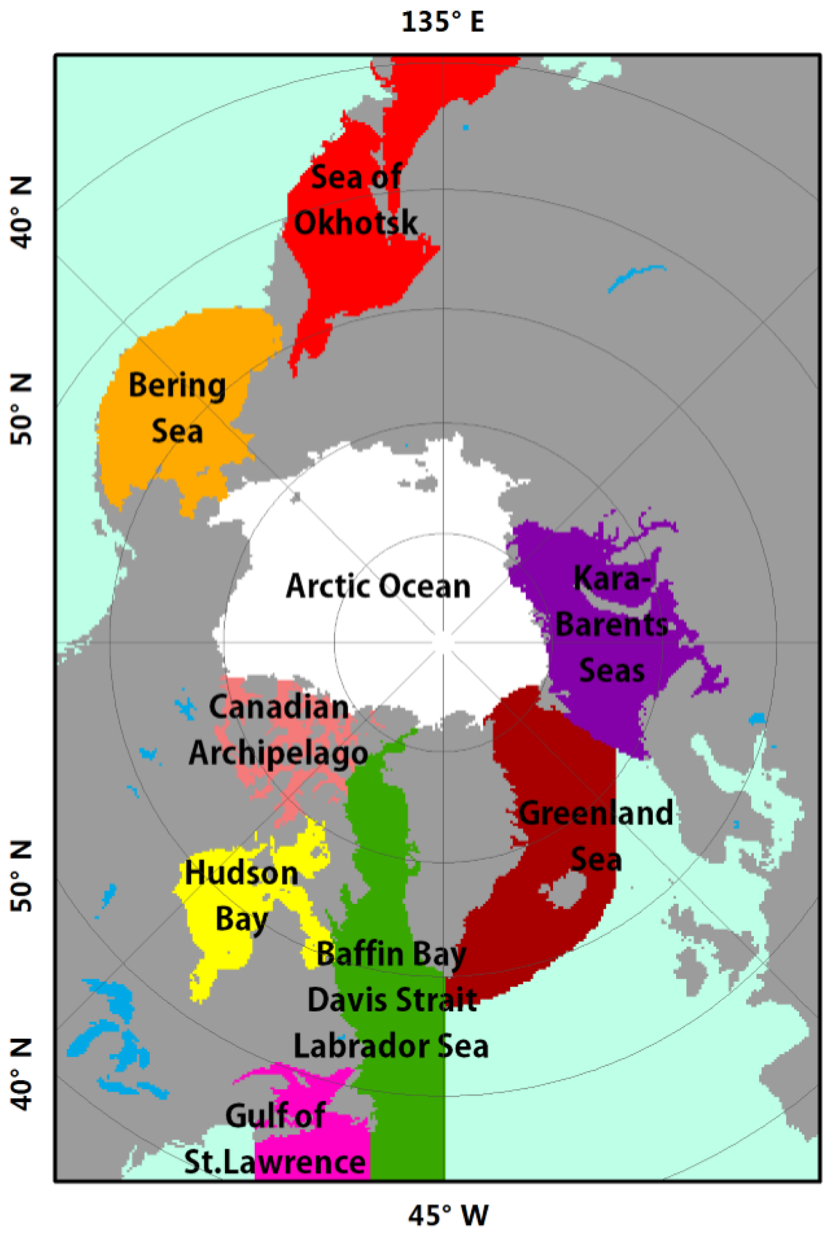
The Barents and Kara Seas area was selected to analyze sea ice changes on a regional scale. Sea ice concentration in this area exhibits very high variability because it is covered by relatively thin seasonal ice [33] impacted by highly variable Atlantic water inflow [34] and atmospheric forcing primarily driven by North Atlantic Oscillation [35,36]. The data for sea ice concentration produced by the NASA Team algorithm, which has been used in many sea ice studies, was obtained from the website of National Snow and Ice Data Center (NSIDC). An enhancement of the algorithm by the NASA Team on sea ice concentration overcomes the problem of a low ice concentration bias associated with surface snow effects. It is calculated based on the brightness temperature difference between 19 and 37 GHz channels obtained from SMMR and SSM/I [11]. We used monthly dataset with a spatial resolution of 0.25 × 0.25 degrees in the polar stereographic projection centered on the North Pole. The Barents and Kara Seas area was delineated using a region mask provided by NSIDC (Figure 1), which consists of 3912 pixels per scene.

As climate factors affecting the changes of sea ice concentration, we used monthly means of ERA-Interim products, which is the latest global climate reanalysis provided by ECMWF. We first investigated possible explanatory variables in relation to temperature, water, radiation, wind, pressure, heat energy, and cloud conditions. Because monthly radiation variables (e.g., surface net solar radiation and surface net thermal radiation) were only provided in forecasted values not in reanalyzed ones, they were not included in our analyses. Wind variables (e.g., wind speed and U/V component), pressure variables (e.g., mean sea level pressure and surface pressure), and heat energy variables (e.g., sensible heat and latent heat) which showed relatively low correlations (|R| < 0.5) to sea ice concentration during 1979–2012 were also excluded. Hence, we divided the remaining explanatory variables into three groups: (1) temperature-related variables including 2-m temperature, 2-m dewpoint temperature, skin temperature, and sea surface temperature; (2) water-related variables including vertical integral of water vapor, total column liquid water, total column water vapor, total column water, and instantaneous moisture flux; and (3) cloud-related variables such as low, medium, and high cloud cover. We finally selected skin temperature, sea surface temperature, total column liquid water, total column water vapor, instantaneous moisture flux, and low cloud cover as appropriate explanatory variables by considering the correlation coefficients to sea ice concentration and multicollinearity between variables within the group.

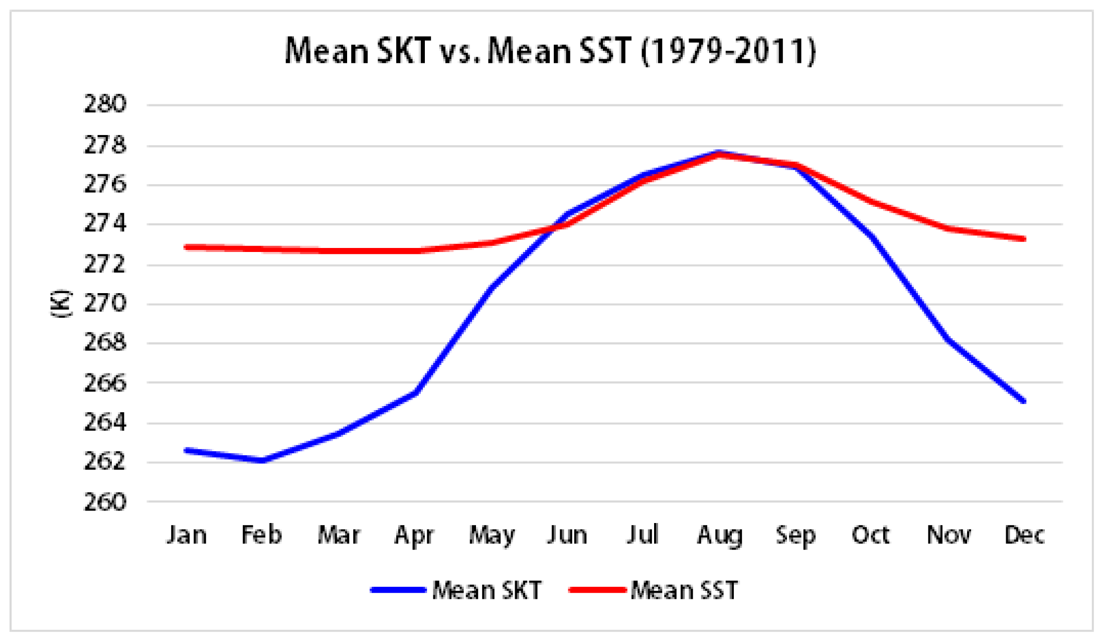
The skin temperature (K) is defined as the temperature of the top skin of the sea (approximately ≤0.01 mm), and the sea surface temperature (K) indicates the temperature of the sea at approximately 20–30 cm depth. The total column liquid water (kg/m²) denotes vertical integral of water in the liquid phase from the ground to the nominal top of the atmosphere expressing the total amount of cloud liquid water, and the total column water vapor (kg/m²) is for the total amount of water vapor in the atmosphere. The instantaneous moisture flux (kg/m²/s) indicates the amount of evaporation for a unit area per second. Low cloud cover (0–1) is the fraction of clouds in the low layer, where the ratio of pressure to surface pressure is >0.8. The ERA-Interim products have been advanced by a data assimilation scheme based on 12 h 4D-Var, which possesses improved model physics, fast radiative transfer model, and better formulation of background error constraint [32]. The data is originally produced with a spatial resolution of 0.75 × 0.75 degrees and can be also provided on the grids of 0.25 × 0.25 and 0.5 × 0.5 degrees through a spatial interpolation. We used the data on the 0.25 × 0.25-degrees grid and its geographic projection with latitude and longitude was converted into the polar stereographic projection in accordance with the NSIDC sea ice products. A set of map projection parameters such as latitude of standard parallel, longitude of central meridian, false easting, and false northing was specified for the conversion [37].

Finally, 408 monthly layers for the 34 years (1979–2012) were aggregated from the NSIDC sea ice products and the ECMWF reanalysis datasets in order to examine the relationships between sea ice concentration and climate factors such as skin temperature, sea surface temperature, total column liquid water, total column water vapor, instantaneous moisture flux, and low cloud cover. Explanatory variables were normalized in the form of z-score calculated as (x_i − χ̄)/σ_x, where x_i is an individual value, χ̄ is the mean, and σ_x is the standard deviation for the entire pixels during 1979–2012. This is because normalized values allow for comparisons among the regression coefficients of explanatory variables even though they originally had different units.

2.2. Statistical Models

A regular regression model is based on the ordinary least squares method, which can be expressed in the Formula:

$$y={\beta }_0+{\beta }_1{x}_1+{\beta }_2{x}_2+\cdots +{\beta }_k{x}_k+\varepsilon$$

(1)

where y is a response variable and x₁ to x_k are explanatory variables. In remote sensing studies, y is generally a remotely sensed variable and x₁ to x_k are environmental variables of interest. β₀ represents the intercept, and β₁ to β_k are the slopes of the relationship between y and x₁ to x_k. The error term ε may include all other factors influencing the response variable y except for the regressors x₁ to x_k. In this study, y is the sea ice concentration and x₁ to x_k are skin temperature, sea surface temperature, total column water, total column liquid water, instantaneous moisture flux, and low cloud cover, respectively. The OLS regression model is often assumed to apply universally over the whole area and the whole period, which implies spatial and temporal stationarities in the relationship between the response and explanatory variables.

Since some environmental phenomena can be explained in terms of temporality or seasonality, the ARIMA model may be useful in explaining complex long-range dataset. In contrast to the OLS approach, the ARIMA model assumes temporal non-stationarity based on the possible differences in the relationships between response and explanatory variables over time [38]. The model is briefly expressed as ARIMA (p,d,q) where parameters p, d, and q are non-negative integers that refer to the order of autoregressive (p), integrated (d), and moving average (q) parts of the model, respectively. Also, seasonal ARIMA model is denoted as ARIMA(p,d,q)(P,D,Q) with additional parameters such as seasonal autoregressive order (P), seasonal differencing order (D), and seasonal moving average order (Q). These parameters can determine the predictability of an ARIMA model and can be optimized by minimizing the criteria such as AIC (Akaike information criterion) and BIC (Bayesian information criterion). A typical seasonal ARIMA model has the following form [39]:

$${(1-B)}^d{(1-B^s)}^D{Y}_t=\mu +\frac{\theta (B){\theta }_s(B^s)}{\phi (B){\phi }_s(B^s)}{a}_t$$

(2)

where B is the backshift operator; Y_t is the time series; μ is the mean term; φ(B) is the non-seasonal autoregressive operator; φ_S(B^S) is the seasonal autoregressive operator; θ(B) is the non-seasonal moving average operator; θ_S(B^S) is the seasonal moving average operator; a_t is the random error. In order to employ the ARIMA method in the time-series modeling with multiple explanatory variables, we can add regressors to an ARIMA equation, which literally adds the regressors to the right-hand-side of the equation.

3. Results and Discussion

3.1. OLS Regression Model Results

Using the monthly data for sea ice concentration and climate variables, we derived OLS regression equations as follows:

$$SIC={\beta }_0+{\beta }_{SKT}SKT+{\beta }_{SST}SST+{\beta }_{TCLW}TCLW+{\beta }_{TCWV}TCWV+{\beta }_{IMF}IMF+{\beta }_{LCC}LCC$$

(3)

where the response variable SIC denotes sea ice concentration, and the explanatory variables SKT, SST, TCLW, TCWV, IMF, and LCC indicate skin temperature, sea surface temperature, total column liquid water, total column water vapor, instantaneous moisture flux, and low cloud cover, respectively. In order to examine seasonal characteristics of the relationships between sea ice concentration and six climate variables, the above equation was built into 12 different versions for each month. Our calibration and validation schemes employed leave-one-out method for the year 2012, 2002, 1992, and 1982: (1) calibration of 33-year dataset except 2012 (for validation of 2012); (2) calibration of 33 year dataset except 2002 (for validation of 2002); (3) calibration of 33-year dataset except 1992 (for validation of 1992); and (4) calibration of 33-year dataset except 1982 (for validation of 1982).

First, monthly means during 1979–2011 were aggregated for each pixel to validate the OLS model for 2012. The p-values of the regression coefficients (β_SKT, β_SST, β_TCLW, β_TCWV, β_IMF, and β_LCC) produced by t-test were <0.01 for almost all cases (

Table 1. Coefficients of the OLS regression models calibrated during 1979–2011. β₀ denotes intercept, and β_SKT, β_SST, β_TCLW, β_TCWV, β_IMF, and β_LCC are the coefficients of skin temperature, sea surface temperature, total column liquid water, total column water vapor, instantaneous moisture flux, and low cloud cover, respectively.

Coefficient	Jan.	Feb.	Mar.	Apr.	May	Jun.	Jul.	Aug.	Sep.	Oct.	Nov.	Dec.
β0	0.595	0.718	0.864	0.739	1.255	1.558	0.749	−0.105	0.851	0.503	0.489	0.470
βSKT	−0.040	−0.077	−0.160	−0.354	−2.344	−0.870	* 0.139	1.049	−2.047	−0.841	−0.290	−0.078
βSST	0.297	0.264	0.260	0.107	0.197	−0.401	−0.377	−0.643	0.349	0.094	0.157	0.339
βTCLW	−0.084	−0.053	0.227	* 0.493	0.854	−0.520	−0.080	−0.163	* 0.009	−0.069	−0.292	−0.126
βTCWV	−0.085	0.081	0.106	−0.051	0.364	0.055	* 0.032	0.265	0.628	0.512	0.339	−0.124
βIMF	0.364	0.363	0.382	0.292	−0.512	−1.216	−0.555	−0.402	−0.296	−0.095	0.210	0.348
βLCC	0.052	0.049	0.059	0.024	−0.041	−0.191	−0.066	0.018	0.013	0.065	0.039	0.085

p-value < 0.01 except for the cases superscripted by ^*.

).

Skin temperature at the top of sea surface had a considerable seasonal variation when compared to the sea surface temperature at 20–30 cm depth (Figure 2). The reason of such variation is caused by the fact that skin temperature is controlled by solar radiation in summer and by atmospheric condition in winter whereas sea surface temperature is influenced by the North Atlantic current all the year round. In addition, seasonal changes of β_SKT and β_SST were quite different (Figure 3) even though both atmospheric and oceanic forcing of sea ice cover could contribute to thermodynamic melting. In warmer months, the skin temperature showed a sharp increase, and such rapid changes might act as a noise leading to the reversion of the regression coefficients: β_SKT abruptly changed to positive in July and August. During the winter season (from October to April), β_SKT and β_SST showed relatively similar values close to zero, which might be due to the weaker thermodynamic effects of skin temperature and sea surface temperature below the freezing point.

Sea ice–cloud interactions and sea ice–water vapor interactions are very complicated since they are associated with many aspects of the energy balance and dynamics in the atmosphere. However, some previous studies, e.g., [40–45] put forward that cloud covers are closely related to the changes in sea ice concentration even if the physical mechanism of effect of cloud warming or cooling on the surface or top of the atmosphere may not be well explained. Although the normalized values of total column liquid water (in clouds) and total column water vapor were very similar throughout the months (Figure 4), β_TCLW and β_TCWV showed somewhat different seasonal patterns (Figure 5). In particular, β_TCLW increased in spring (March, April, and May) but dropped to negative values in June when the melting starts. It can be assumed that the warming or cooling effects of clouds were differently applied according to the month or season and led to such a unique pattern [44,45].

The R² values for explanatory power were very high in colder months (mostly >0.95 from October to May), but were relatively low in warmer months (approximately 0.8 from June to September) (

Table 2. R² in the OLS regression models calibrated for each month during 1979–2011.

Month	Jan.	Feb.	Mar.	Apr.	May	Jun.	Jul.	Aug.	Sep.	Oct.	Nov.	Dec.	Average
R2	0.988	0.989	0.981	0.975	0.948	0.908	0.836	0.782	0.880	0.964	0.977	0.980	0.934

) partly because of the low correlation coefficients of explanatory variables in the months (

Table 3. Pearson correlation coefficients (R) of the six explanatory variables for the sea ice concentration. They were calculated from the averages of the normalized variables during 1979–2011.

Pearson R	Jan.	Feb.	Mar.	Apr.	May	Jun.	Jul.	Aug.	Sep.	Oct.	Nov.	Dec.
SKT	−0.979	−0.966	−0.965	−0.969	−0.973	−0.941	−0.850	−0.657	−0.583	−0.800	−0.932	−0.972
SST	−0.847	−0.880	−0.890	−0.896	−0.824	−0.727	−0.570	−0.390	−0.336	−0.511	−0.663	−0.758
TCLW	−0.833	−0.809	−0.816	−0.849	−0.873	−0.852	−0.799	−0.628	−0.552	−0.740	−0.852	−0.861
TCWV	−0.874	−0.855	−0.863	−0.897	−0.913	−0.874	−0.814	−0.648	−0.578	−0.760	−0.874	−0.893
IMF	0.976	0.987	0.986	0.978	0.942	0.878	0.728	0.515	0.448	0.666	0.833	0.917
LCC	0.834	0.851	0.864	0.888	0.844	0.753	0.621	0.442	0.385	0.590	0.731	0.789

p-value < 0.01 for all cases.

). Such low correlations may be related to the atmospheric and oceanic effects on the time lag of thermodynamic melting in warmer months [26,46]. Then, we prepared satellite-observed monthly sea ice concentration in the Barents and Kara Seas in 2012 (Figure 6) for the validation of the OLS regression models calibrated during 1979–2011. We derived the values of the monthly concentration of sea ice for each pixel of the Barents and Kara Seas in 2012 (Figure 7) and compared them with the NSIDC satellite data to examine the spatial and temporal distributions of prediction errors (Figure 8). The pixels with greater errors overestimated or underestimated were found according to months. This implies a time-series approach based on temporally varying relationships may help diminish the prediction errors in the study area. The results of validation were presented in terms of mean bias and monthly root mean square error (RMSE) in

Table 4. Validation of monthly sea ice concentration in 2012 using the OLS regression models calibrated for each month during 1979–2011. The values for the entire pixels were aggregated.

Month	Jan.	Feb.	Mar.	Apr.	May	Jun.	Jul.	Aug.	Sep.	Oct.	Nov.	Dec.	Average
Bias	0.118	0.124	0.099	−0.035	0.154	−0.396	−0.013	−0.047	−0.091	0.014	0.062	0.020	0.001
RMSE	0.205	0.251	0.176	0.214	0.344	0.514	0.117	0.107	0.154	0.072	0.115	0.121	0.199

.

In addition to year 2012, the validations were conducted for the years 2002, 1992, and 1982. The R² of the OLS regression models were shown in

Table 5. R² in the OLS regression models calibrated for validating the monthly sea ice concentration in 2002, 1992, and 1982.

Month	Jan.	Feb.	Mar.	Apr.	May	Jun.	Jul.	Aug.	Sep.	Oct.	Nov.	Dec.	Average
R2 (2002)	0.988	0.989	0.981	0.975	0.945	0.907	0.838	0.787	0.870	0.962	0.977	0.979	0.933
R2 (1992)	0.988	0.989	0.981	0.973	0.947	0.910	0.837	0.782	0.864	0.961	0.977	0.980	0.932
R2(1982)	0.988	0.989	0.981	0.975	0.947	0.906	0.832	0.776	0.866	0.960	0.977	0.980	0.931

, and the mean bias and RMSE were presented in

Table 6. Validations of sea ice concentration in 2002, 1992, and 1982 using the OLS regression models. The values for the entire pixels were aggregated.

Month	Jan.	Feb.	Mar.	Apr.	May	Jun.	Jul.	Aug.	Sep.	Oct.	Nov.	Dec.	Average
Bias (2002)	−0.040	−0.070	−0.032	0.154	0.049	0.144	0.027	0.055	−0.061	−0.016	0.048	−0.043	0.018
Bias (1992)	0.017	0.008	0.091	−0.165	0.045	0.209	0.077	−0.017	0.132	−0.087	0.007	−0.058	0.022
Bias (1982)	−0.036	0.051	0.025	0.034	−0.099	0.359	−0.053	−0.043	−0.063	−0.026	0.014	−0.015	0.012
RMSE (2002)	0.106	0.135	0.124	0.334	0.234	0.234	0.187	0.175	0.093	0.138	0.125	0.093	0.165
RMSE (1992)	0.111	0.112	0.152	0.267	0.271	0.420	0.198	0.161	0.189	0.187	0.107	0.149	0.193
RMSE (1982)	0.124	0.111	0.098	0.125	0.249	0.727	0.172	0.176	0.116	0.086	0.148	0.130	0.188

, which were not significantly different from those of year 2012. Also, the seasonal patterns of the six regression coefficients were almost same as those in 2012. Given that climatic characteristics might vary according to individual years, the six explanatory variables can be considered representative to predict sea ice concentration under the changes of atmospheric and oceanic conditions.

3.2. Time-Series Model Results

Unlike the OLS regression, the ARIMA model can apply for each pixel containing a multivariate time series of the sea ice concentration and its six explanatory variables (Figure 9). We employed the R “forecast” library for optimizing the model parameters of ARIMA(p,d,q)(P,D,Q) with the six regressors. The calibration period was set as between January 1979 and the month right before the predicted month: for example, a time series from January 1979 to April 2012 was used in predicting May 2012. Figure 10 shows the spatial distribution of estimated values of sea ice concentration by the ARIMA models, and Figure 11 is the map of validation accuracies. The RMSE of the ARIMA models was summarized in

Table 7. RMSE improvements of monthly sea ice concentration in 2012 using the ARIMA models calibrated by the time series for each pixel. The improvements were calculated by subtracting the RMSE of ARIMA model from that of OLS model in Table 4. The values for the entire pixels were aggregated.

Month	Jan.	Feb.	Mar.	Apr.	May	Jun.	Jul.	Aug.	Sep.	Oct.	Nov.	Dec.	Average
RMSE	0.100	0.159	0.082	0.093	0.144	0.182	0.166	0.094	0.100	0.170	0.090	0.098	0.123
Improvement	0.105	0.092	0.094	0.121	0.200	0.332	−0.049	0.013	0.054	−0.098	0.025	0.023	0.076

, and the improvements against the OLS models were illustrated in Figure 12. Particularly for May and June when the RMSE of the OLS model were worst (0.344 in May and 0.514 in June), the ARIMA model shows considerable improvements, by 0.2 and 0.332, respectively. The average improvement of RMSE was 0.076, which reveals the effect of time-series modeling given that the range of sea ice concentration is between 0 and 1. In addition, the validation accuracies of the ARIMA were relatively stable throughout the months: the standard deviation of monthly RMSE was 0.036 for the ARIMA, but 0.119 for the OLS model. However, the RMSE slightly worsened for two months (by 0.049 in July and by 0.098 in October), which might be recovered by using another time-series approach like vector autoregression.

4. Conclusions

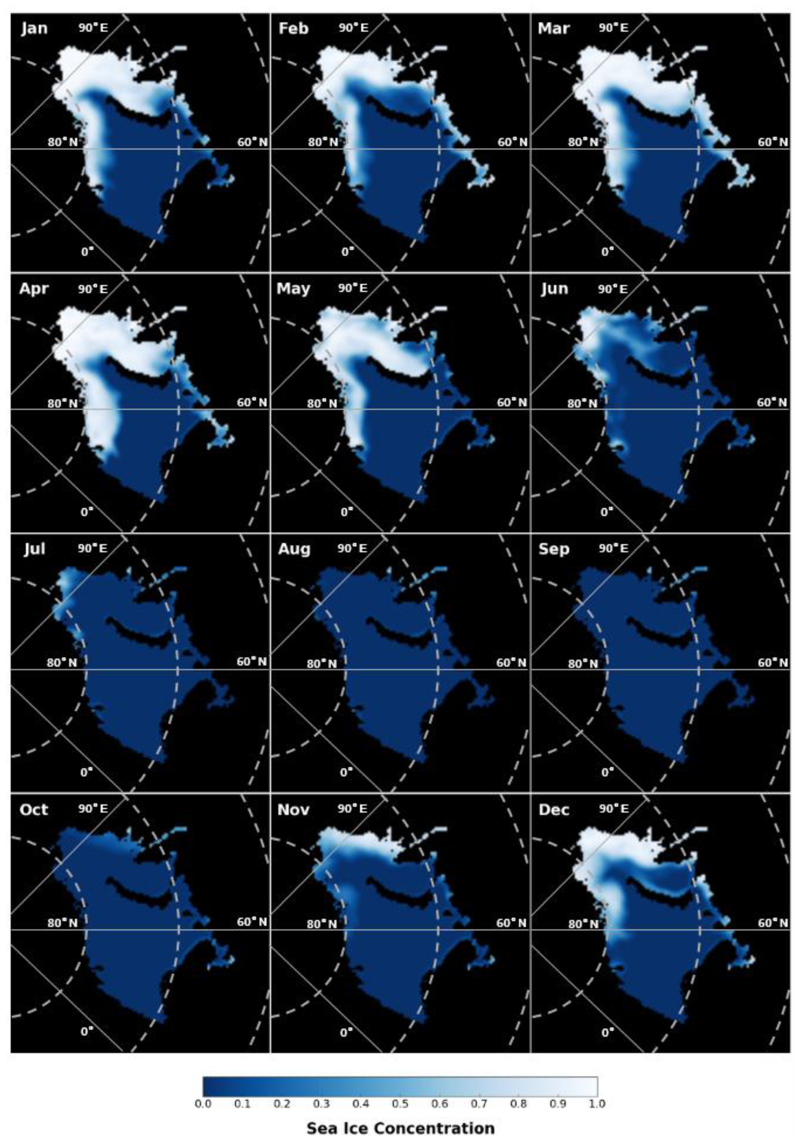
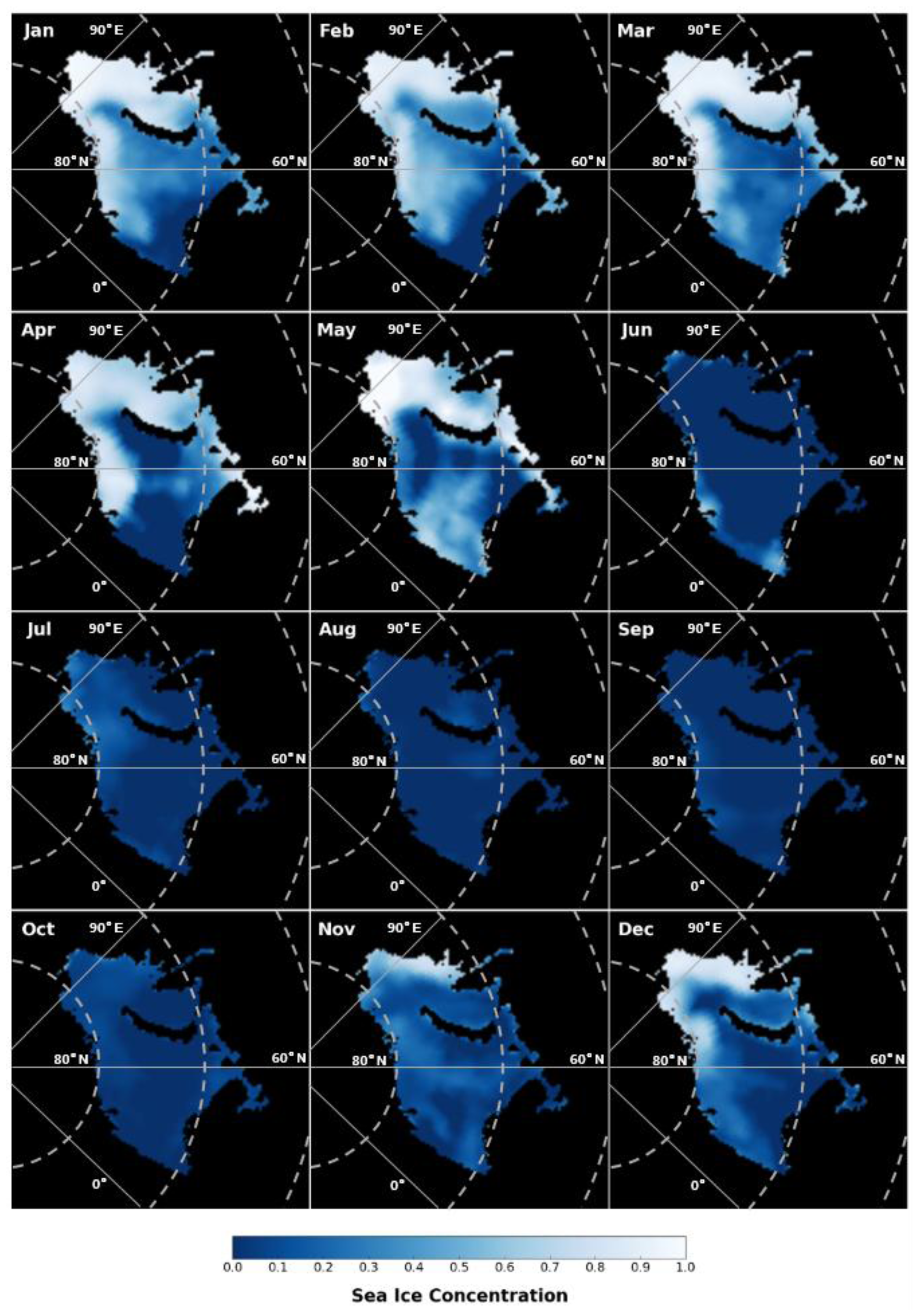
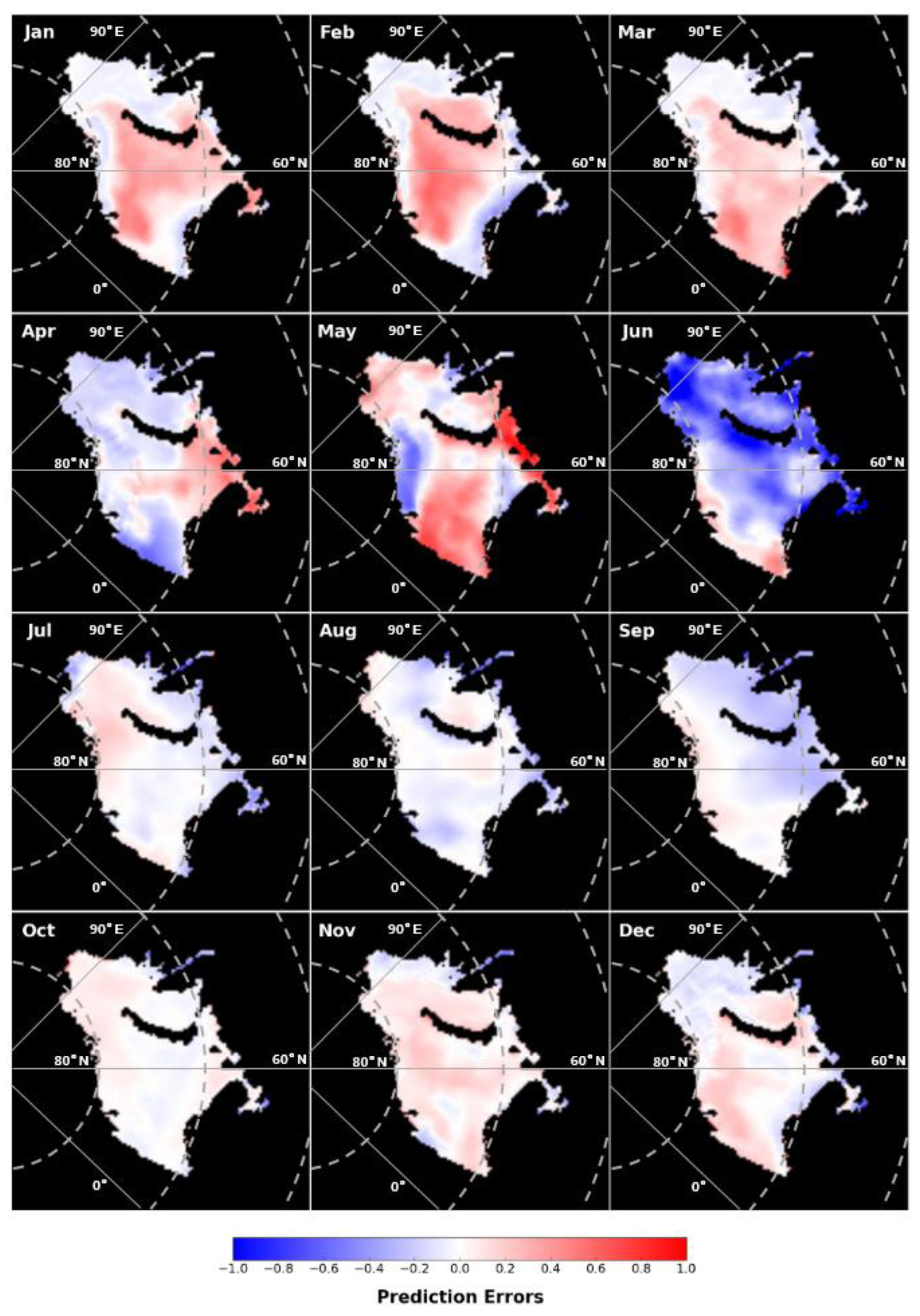
In this paper, we described the statistical modeling of sea ice concentration in relation to climatic factors, using satellite imagery and climate reanalysis data for the Barents and Kara Seas during 1979–2012. The OLS regression model summarized the whole years and provided information about overall climatological characteristics in the relationships between sea ice concentration and climate variables. In particular, the ARIMA method was first introduced to statistical model for sea ice concentration and it helped improve prediction accuracies because the time series of the sea ice concentration is such a long-range dataset that the relationships may not be explained by a single equation of the OLS regression. We found that temporally varying relationships between sea ice concentration and the climate factors such as skin temperature, sea surface temperature, total column liquid water, total column water vapor, instantaneous moisture flux, and low cloud cover were modeled by the ARIMA method, which resulted in better prediction accuracies. The RMSE improvement was 0.076 on average (0.199 by OLS and 0.123 by ARIMA), and the prediction accuracies of the ARIMA were relatively stable throughout the months. Our improved statistical approach with the ARIMA method may be worth consideration when forecasting future sea ice concentration using the climate data provided by general circulation models (GCM).

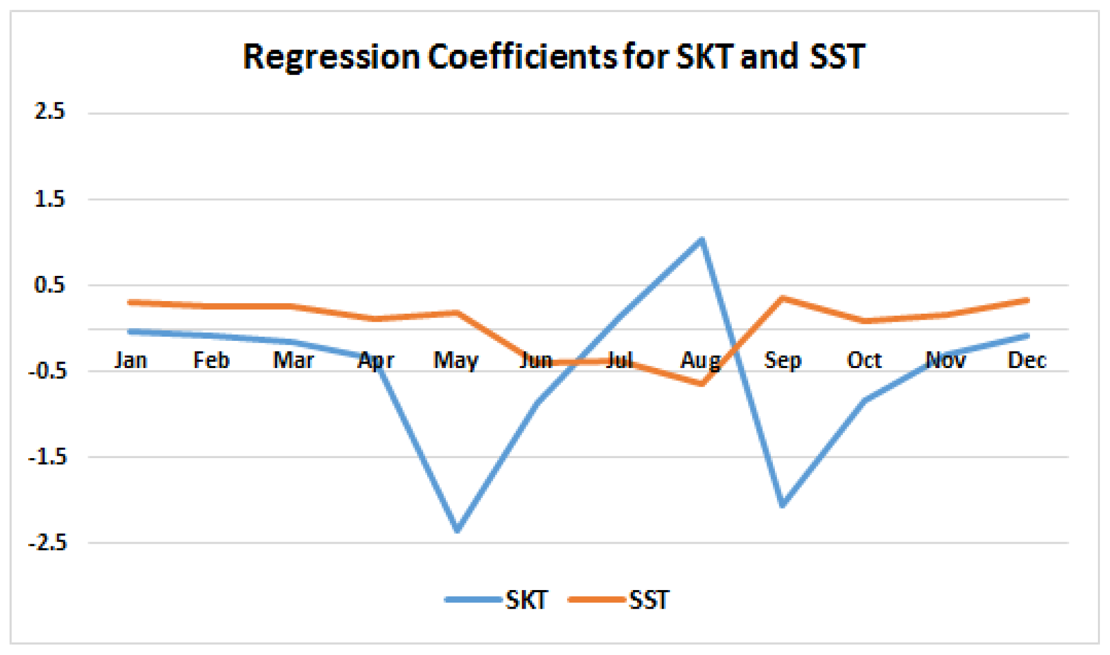
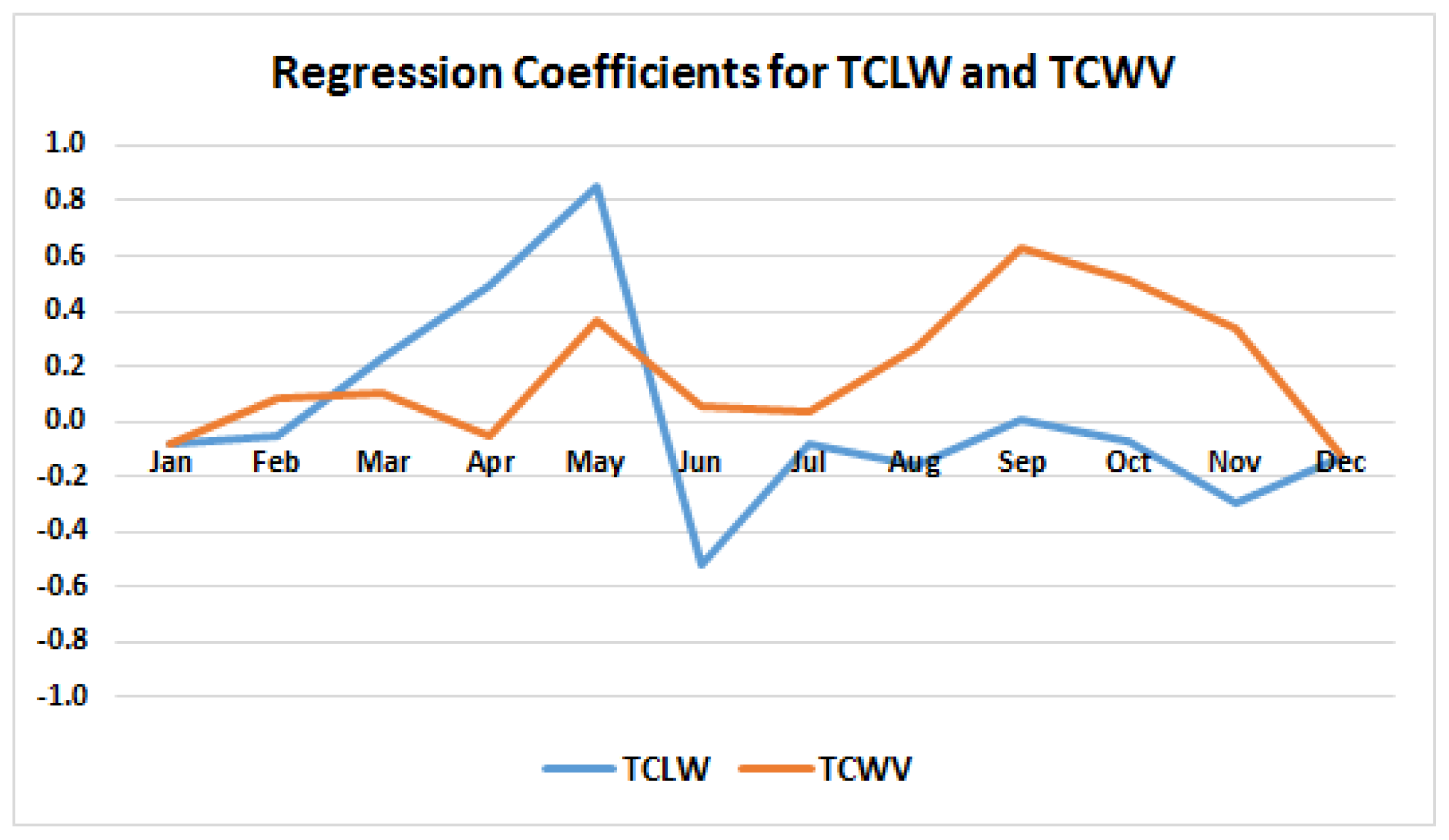
In addition, some unique characteristics of the climate factors in relation to sea ice concentration were found during the analyses. In July and August when the ice melts, β_SKT showed abrupt positive values presumably because rapid increases of skin temperature might act as a noise in the regression coefficients. During winter, β_SKT and β_SST showed relatively similar values close to zero partly because of the weaker thermodynamic effects of skin temperature and sea surface temperature below the freezing point. Unlike the total column water vapor, the total column liquid water (in clouds) brought about a peculiar seasonal pattern of β_TCLW because the warming or cooling effects of clouds were applied differently according to season, which will require further investigations to understand the details. Those results may be useful in better understanding the physical mechanism and in improving the statistical model.

Our result derived from limited number of explanatory variables may not be applied universally when considering the complex climate change system. Therefore, additional explanatory variables related to solar radiation [47], atmospheric refractivity [13], and surface roughness [48] should be incorporated in the statistical models for further improvements in prediction accuracies. In addition, we did not identify the time-lag between explanatory variables and sea ice concentration, but given that previous studies have reported the time-lag in melt onset or freeze-up [46], a closer examination of this will be necessary for improving the time-series modeling.

References

1. Deser, C.; Walsh, J.E.; Timlin, M.S. Arctic sea ice variability in the context of recent atmospheric circulation trends. J. Clim 2000, 13, 617–633. [Google Scholar]
2. Comiso, J.C. Satellite-observed variability and trend in sea-ice extent, surface temperature, albedo and clouds in the Arctic. Ann. Glaciol 2001, 33, 457–473. [Google Scholar]
3. Laxon, S.; Peacock, N.; Smith, D. High interannual variability of sea ice thickness in the Arctic region. Nature 2003, 425, 947–950. [Google Scholar]
4. Parkinson, C.L.; Cavalieri, D.J.; Gloersen, P.; Zwally, H.J.; Comiso, J.C. Arctic sea ice extents, areas, and trends, 1978–1996. J. Geophy. Res 1999, 104, 20837–20856. [Google Scholar]
5. Aagaard, K.; Carmack, E.C. The role of sea ice and other fresh water in the Arctic circulation. J. Geophy. Res 1989, 94, 14485–14498. [Google Scholar]
6. Overland, J.E.; Wang, M. Large-scale atmospheric circulation changes associated with the recent loss of Arctic sea ice. Tellus 2010, 62, 1–9. [Google Scholar]
7. Vinnikov, K.Y.; Robock, A.; Stouffer, R.J.; Walsh, J.E.; Parkinson, C.L.; Cavalieri, D.J.; Mitchell, J.F.B.; Garrett, D.; Zakharov, V.F. Global warming and northern Hemisphere sea ice extent. Science 1999, 286, 1934–1937. [Google Scholar]
8. Alexander, M.A.; Bhatt, U.S.; Walsh, J.E.; Timlin, M.S.; Miller, J.S.; Scott, J.D. The atmospheric response to realistic Arctic sea ice anomalies in an AGCM during winter. J. Clim 2004, 17, 890–905. [Google Scholar]
9. Comiso, J.C. Sea ice effective microwave emissivities from satellite passive microwave and infrared observations. J. Geophy. Res 1983, 88, 7686–7704. [Google Scholar]
10. Cavalieri, D.J.; Parkinson, C.L.; Gloersen, P.; Comiso, J.C.; Zwally, H.J. Deriving long-term time series of sea ice cover from satellite passive-microwave multisensor data sets. J. Geophy. Res 1999, 104, 15803–15814. [Google Scholar]
11. Markus, T.; Cavalieri, D.J. An enhancement of the NASA team sea ice algorithm. IEEE Trans. Geosci. Remote 2000, 38, 1387–1398. [Google Scholar]
12. Comiso, J.C.; Nishio, F. Trends in the sea ice cover using enhanced and compatible AMSR-E, SSM/I, and SMMR data. J. Geophy. Res 2008, 113, C02S07. [Google Scholar]
13. Hong, S.; Shin, I. Global trends of sea ice: Small-scale roughness and refractive index. J. Clim 2010, 23, 4669–4676. [Google Scholar]
14. Hong, S.; Shin, I.; Byun, Y.; Seo, H.; Kim, Y. Analysis of sea ice surface properties using ASH and Hong approximations in passive satellite microwave remote sensing. Remote Sens. Lett 2014, 5, 139–147. [Google Scholar]
15. Francis, J.A.; Chan, W.; Leathers, D.J.; Miller, J.R.; Veron, D.E. Winter Northern Hemisphere weather patterns remember summer Arctic sea-ice extent. Geophys. Res. Lett 2000, 36, L07503. [Google Scholar]
16. Wang, M.; Overland, J.E. A sea ice free summer Arctic within 30 years? Geophys. Res. Lett 2009, 36, L07502. [Google Scholar]
17. Wang, M.; Overland, J.E. A sea ice free summer Arctic within 30 years: An update from CMIP5 models. Geophys. Res. Lett 2012, 39, L18501. [Google Scholar]
18. Drobot, S.D. Using remote sensing data to develop seasonal outlooks for Arctic regional sea-ice minimum extent. Remote Sens. Environ 2007, 111, 136–147. [Google Scholar]
19. Kattsov, V.M.; Ryabinin, V.E.; Overland, J.E.; Serreze, M.C.; Visbeck, M.; Walsh, J.E.; Meier, W.; Zhang, X. Arctic sea-ice change: A grand challenge of climate science. J. Glaciol 2010, 56, 1115–1121. [Google Scholar]
20. Drobot, S.; Maslanik, J. A practical method for long-range forecasting of ice severity in the Beaufort Sea. Geophys. Res. Lett 2002, 29, 1–4. [Google Scholar]
21. Drobot, S. Long-range statistical forecasting of ice severity in the Beaufort–Chukchi Sea. Weather Forecast 2003, 18, 1161–1176. [Google Scholar]
22. Drobot, S.D.; Maslanik, J.A.; Fowler, C. A long-range forecast of Arctic summer sea-ice minimum extent. Geophys. Res. Lett 2006, 33, L10501. [Google Scholar]
23. Lindsay, R.W.; Zhang, J.; Schweiger, A.J.; Steele, M.A. Seasonal predictions of ice extent in the Arctic Ocean. J. Geophy. Res 2008, 113, C02023. [Google Scholar]
24. Årthun, M.; Eldevik, T.; Smedsrud, L.H.; Skagseth, Ø.; Ingvaldsen, R.B. Quantifying the influence of Atlantic heat on Barents sea ice variability and retreat. J. Clim 2012, 25, 4736–4743. [Google Scholar]
25. Pavlova, O.; Pavlov, V.; Gerland, S. The impact of winds and sea surface temperatures on the Barents Sea ice extent: A statistical approach. J. Mar. Syst 2014, 130, 248–255. [Google Scholar]
26. Tivy, A.; Howell, S.E.L.; Alt, B.; Yackel, J.J.; Carrieres, T. Origins and levels of seasonal forecast skill for sea ice in Hudson Bay using canonical correlation analysis. J. Clim 2011, 24, 1378–1395. [Google Scholar]
27. Chapman, W.L.; Walsh, J.E. Recent variations of sea ice and air temperature in high latitudes. Bull. Amer. Meteor. Soc 1993, 74, 33–47. [Google Scholar]
28. Hansen, J.; Ruedy, R.; Sato, M.; Lo, K. Global surface temperature change. Rev. Geophys 2010, 48, RG4004. [Google Scholar]
29. Barnston, A.G. Linear statistical short-term climate predictive skill in the Northern Hemisphere. J. Clim 1994, 7, 1513–1564. [Google Scholar]
30. Maslanik, J.; Drobot, S.; Fowler, C.; Emery, W.; Barry, R. On the Arctic climate paradox and the continuing role of atmospheric circulation in affecting sea ice conditions. Geophys. Res. Lett 2007, 34, L03711. [Google Scholar]
31. Zhang, J.; Lindsay, R.; Steele, M.; Schweiger, A. What drove the dramatic retreat of arctic sea ice during summer 2007? Geophys. Res. Lett 2008, 35, L11505. [Google Scholar]
32. Dee, D.P.; Uppala, S.M.; Simmons, A.J.; Berrisford, P.; Poli, P.; Kobayashi, S.; Andrae, U.; Balmaseda, M.A.; Balsamo, G.; Bauer, P.; et al. The ERA-Interim reanalysis: configuration and performance of the data assimilation system. Q. J. R. Meteorol. Soc 2011, 137, 553–597. [Google Scholar]
33. Rothrock, D.A.; Yu, Y.; Maykut, G.A. Thinning of the Arctic sea-ice cover. Geophys. Res. Lett 1999, 26, 3469–3472. [Google Scholar]
34. Schauer, U.; Loeng, H.; Rudels, B.; Ozhigin, V.K.; Dieck, W. Atlantic water flow through the Barents and Kara Seas. Deep Sea Res. I 2002, 49, 2281–2298. [Google Scholar]
35. Hurrell, J.W. Decadal trends in the North Atlantic Oscillation: Regional temperatures and precipitation. Science 1995, 269, 676–679. [Google Scholar]
36. Sorteberg, A.; Kvingedal, B. Atmospheric forcing on the Barents Sea winter ice extent. J. Clim 2006, 19, 4772–4784. [Google Scholar]
37. Geomatics Guidance Note Number 7 Part 2: Coordinate Conversions and Transformations Including Formulas. Available online: http://www.epsg.org/guides/docs/g7-2.pdf (accessed on 11 June 2014).
38. Tiao, G.C.; Box, G.E.P. Modeling multiple time series with applications. J. Am. Stat. Assoc 1981, 76, 802–816. [Google Scholar]
39. Box, G.E.P.; Jenkins, G.M. Time Series Analysis: Forecasting and Control; Holden-Day Inc.: San Francisco, CA, USA, 1976. [Google Scholar]
40. Wang, X.; Key, J.R. Arctic surface, cloud, and radiation properties based on the AVHRR Polar Pathfinder dataset. Part II: Recent trends. J. Clim 2005, 18, 2575–2593. [Google Scholar]
41. Liu, Y.; Key, J.R.; Francis, J.A.; Wang, X. Possible causes of decreasing cloud cover in the Arctic winter, 1982–2000. Geophys. Res. Lett 2007, 34, L14705. [Google Scholar]
42. Schweiger, A.J.; Lindsay, R.W.; Vavrus, S.; Francis, J.A. Relationships between Arctic sea ice and clouds during autumn. J. Clim 2008, 21, 4799–4810. [Google Scholar]
43. Liu, Y.; Key, J.R.; Wang, X. Influence of changes in sea ice concentration and cloud cover on recent Arctic surface temperature trends. Geophys. Res. Lett 2009, 36, L20710. [Google Scholar]
44. Eastman, R.; Warren, S.G. Arctic cloud changes from surface and satellite observations. J. Clim 2010, 23, 4233–4242. [Google Scholar]
45. Liu, Y.; Key, J.R.; Liu, Z.; Wang, X.; Vavrus, S.J. A cloudier Arctic expected with diminishing sea ice. Geophys. Res. Lett 2012, 39, L05705. [Google Scholar]
46. Wang, J.; Mysak, L.A.; Ingram, R.G. Interannual variability of sea-ice cover in Hudson bay, Baffin bay and the Labrador sea. Atmos.-Ocean 1994, 32, 421–447. [Google Scholar]
47. Frey, K.E.; Perovich, D.K.; Light, B. The spatial distribution of solar radiation under a melting Arctic sea ice cover. Geophy. Res. Lett 2011, 38, L22501. [Google Scholar]
48. Hong, S. Surface roughness and polarization ratio in microwave remote sensing. Int. J. Remote Sens 2010, 31, 2709–2716. [Google Scholar]
Figure 1. The regional mask around the Arctic provided by the National Snow and Ice Data Center (NSIDC). It includes Arctic Ocean, Barents and Kara Seas, Greenland Sea, Baffin Bay/Davis Strait/Labrador Sea, Gulf of St. Lawrence, Hudson Bay, Canadian Archipelago, Bering Sea, and Sea of Okhotsk.
Remotesensing 06 05520f1
Figure 2. Monthly mean skin temperature (SKT) and sea surface temperature (SST) during 1979–2011. The values for the entire pixels were aggregated.
Remotesensing 06 05520f2
Figure 3. Monthly changes of regression coefficients for skin temperature (SKT) and sea surface temperature (SST). They were calculated from the averages of the normalized variables during 1979–2011.
Remotesensing 06 05520f3
Figure 4. Monthly mean total column liquid water (TCLW) and total column water vapor (TCWV) during 1979–2011. The values for the entire pixels were aggregated.
Remotesensing 06 05520f4
Figure 5. Monthly changes of regression coefficients for the total column liquid water (TCLW) and the total column water vapor (TCWV) during 1979–2011.
Remotesensing 06 05520f5
Figure 6. Satellite-observed monthly sea ice concentration in the Barents and Kara Seas in 2012.
Remotesensing 06 05520f6
Figure 7. Monthly sea ice concentration predicted by the OLS regression models for the Barents and Kara Seas in 2012.
Remotesensing 06 05520f7
Figure 8. Prediction errors of the OLS regression models for the Barents and Kara Seas in 2012.
Remotesensing 06 05520f8
Figure 9. Conceptual framework of the ARIMA models to incorporate temporally varying relationships between sea ice concentration and climate variables.
Remotesensing 06 05520f9
Figure 10. Monthly sea ice concentration predicted by the ARIMA models for the Barents and Kara Seas in 2012.
Remotesensing 06 05520f10
Figure 11. Prediction errors of the ARIMA regression models for the Barents and Kara Seas in 2012.
Remotesensing 06 05520f11
Figure 12. Prediction accuracy improvements by the ARIMA models for Barents and Kara Seas in 2012.
Remotesensing 06 05520f12