A Bayesian Based Method to Generate a Synergetic Land-Cover Map from Existing Land-Cover Products

Abstract

Global land cover is an important parameter of the land surface and has been derived by various researchers based on remote sensing images. Each land cover product has its own disadvantages and limitations. Data fusion technology is becoming a notable method to fully integrate existing land cover information. In this paper, we developed a method to generate a synergetic global land cover map (synGLC) based on Bayes theorem. A state probability vector was defined to precisely and quantitatively describe the land cover classification of every pixel and reduce the errors caused by legends harmonization and spatial resampling. Simple axiomatic approaches were used to generate the prior land cover map, in which pixels with high consistency were regarded to be correct and then used as benchmark to obtain posterior land cover map. Validation results show that our hybrid land cover map (synGLC, the dataset is available on request) has the best overall performance compared with the existing global land cover products. Closed shrub-lands and permanent wetlands have the highest uncertainty in our fused land cover map. This novel method can be extensively applied to fusion of land cover maps with different legends, spatial resolutions or geographic ranges.

1. Introduction

Land cover data describes physical material at the surface of the earth. It has great impacts on surface energy, carbon cycle, water balance and consequences of land use and land cover change [1–4]. Also, it is a basic parameter for many land surface models, such as Ecosystem-Atmosphere Simulation Scheme [5] and the Common Land Model [6]. Reliable and accurate land cover data provides key information for relevant environmental researches [7].

As shown in

Table 1. Land cover datasets used in this study.

Dataset	Coverage Year	Spatial Resolution	Legend	Website
UMDLC	1981–1994	1 km	14 classes	[9]
GLCC	1992–1993	1 km	IGBP	[11]
GLC2000	2000	1/112 degree	FAO LCCS	[13]
MCD12Q1	2005	500 m	IGBP	[16]
GlobCover	2009	1/360 degree	UN LCCS	[18]

, various global land cover datasets have been produced based on remote sensing data, including Global Land Cover Classification [8,9] from University of Maryland Department of Geography (UMDLC), Global Land Cover Characterization (GLCC) Data Base [10,11], Global Land Cover map for year 2000 (GLC2000) from the European Commission Joint Research Centre [12,13], the Moderate-Resolution Imaging Spectroradiometer (MODIS) global land cover map products (MCD12Q1) developed by Boston University and coordinated by the MODIS Land Team from the National Aeronautics and Space Administration [14–16], and Global Land Cover Map (GlobCover) from the European Space Agency (ESA) in cooperation with an international network of partners [17,18].

GLCC was developed through a continent-by-continent unsupervised classification of 1-km monthly Advanced Very High Resolution Radiometer (AVHRR) Normalized Difference Vegetation Index (NDVI) composites covering a 12-month period (April 1992–March 1993). UMDLC was based on data from the AVHRR, using the classification tree approach [8]. GLC2000 was produced based on daily global data acquired by the Vegetation instrument on board the Systeme Probatoire d’Observation de la Terre (SPOT) 4 satellite [12]. MCD12Q1 was derived from observations spanning a year’s input of Terra- and Aqua-MODIS data. GlobCover2009 was generated using an automated processing chain from the 300-m Medium Resolution Imaging Spectrometer Instrument (MERIS) time series.

Previous inter-comparisons of these data-sets [19–22] revealed marked disagreements and uncertainties among them. Several researchers tried to produce a hybrid global land cover map by fusion of existing land cover products [7,23,24]. See and Fritz [24] firstly produced a hybrid land cover map by fusion of the GLC2000 and MODIS products. Jung et al. [23] presented a method that merged existing products into a new joint 1-km global land cover product with improved characteristics for the carbon cycle models. However, the individual strengths and weaknesses of the products were not considered, and did not provide validation or data quality assessment. Fritz et al. [25] then generated a synergy cropland map in sub-Saharan Africa from five global land cover products, which requires subjective ranking by experts and does not consider legends conversion. Perez-Hoyos et al. [7] developed a general framework of building a hybrid land-cover map for Europe using four land-cover data-sets. This approach can be applied to any set of existing products; however it requires enough training data, which limits its application to the global scale.

The objective of this study is to produce a hybrid global land cover map by making use of all existing global land cover datasets with different legends and different spatial resolutions. A novel technique based on Bayes theorem was developed. Classification of each pixel in land cover map was represented by discrete probability distribution which more precisely describes state of land cover. The hybrid global land cover dataset was produced as the posterior distribution of a prior global land cover map.

2. Materials

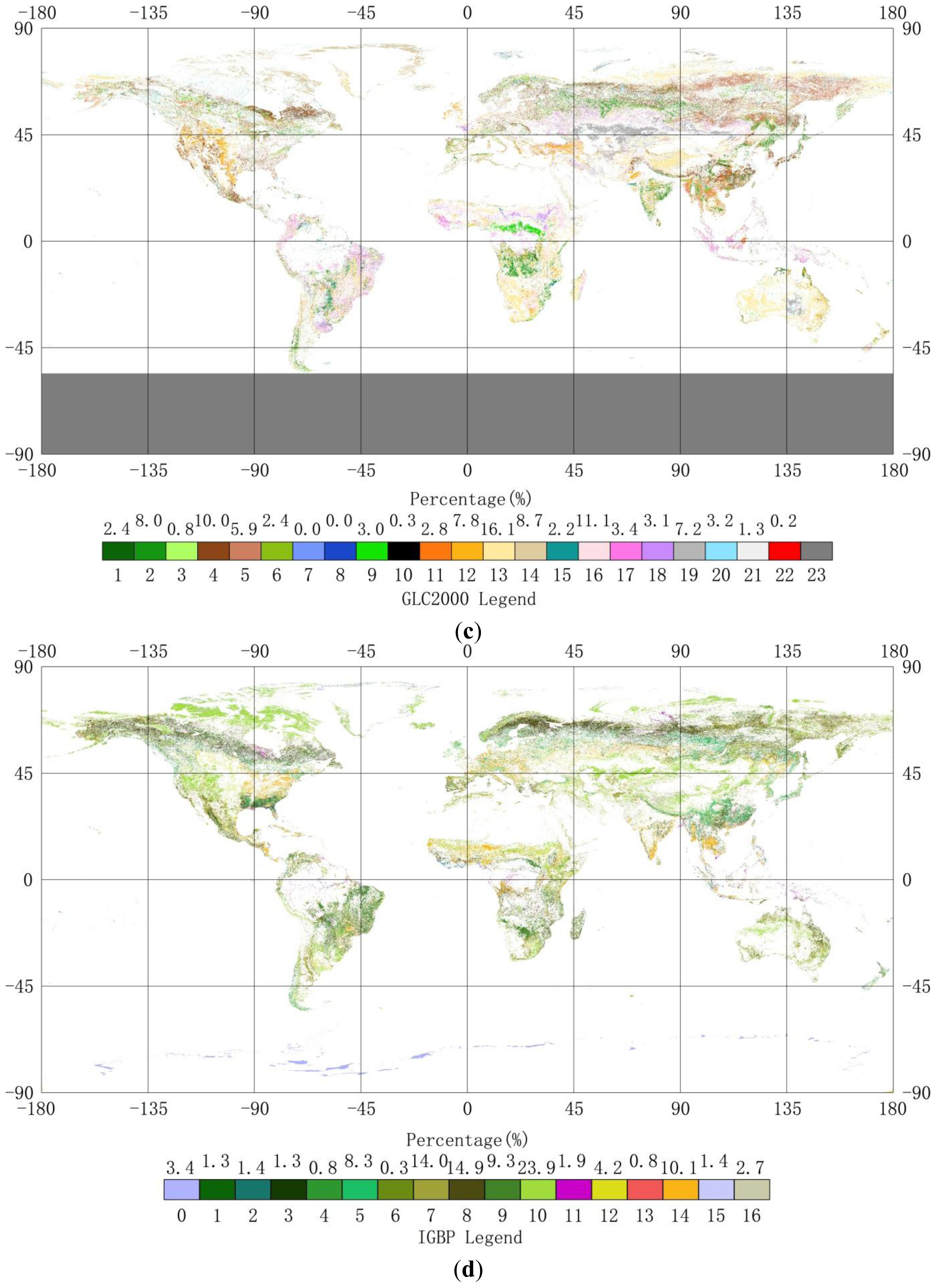
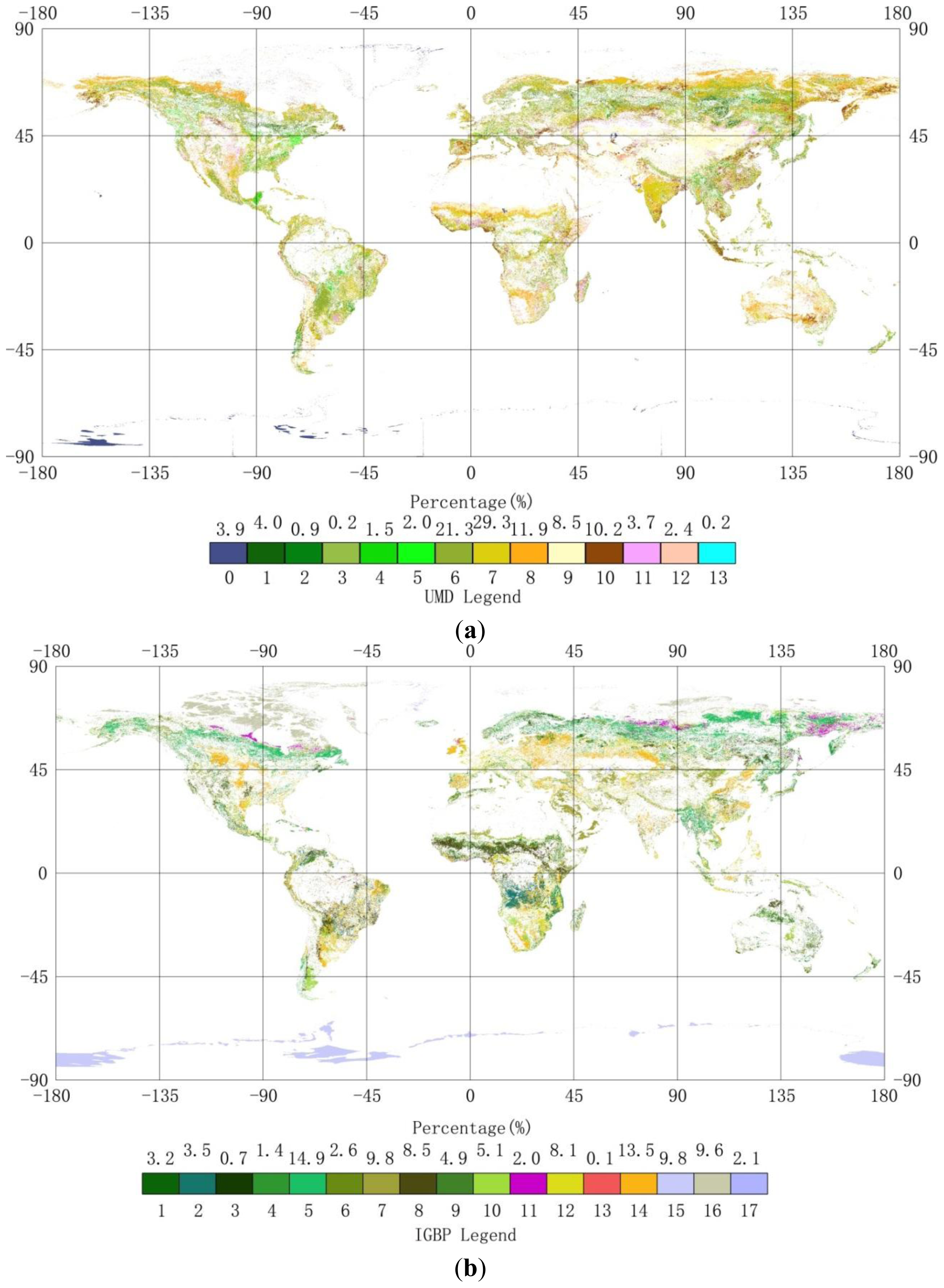
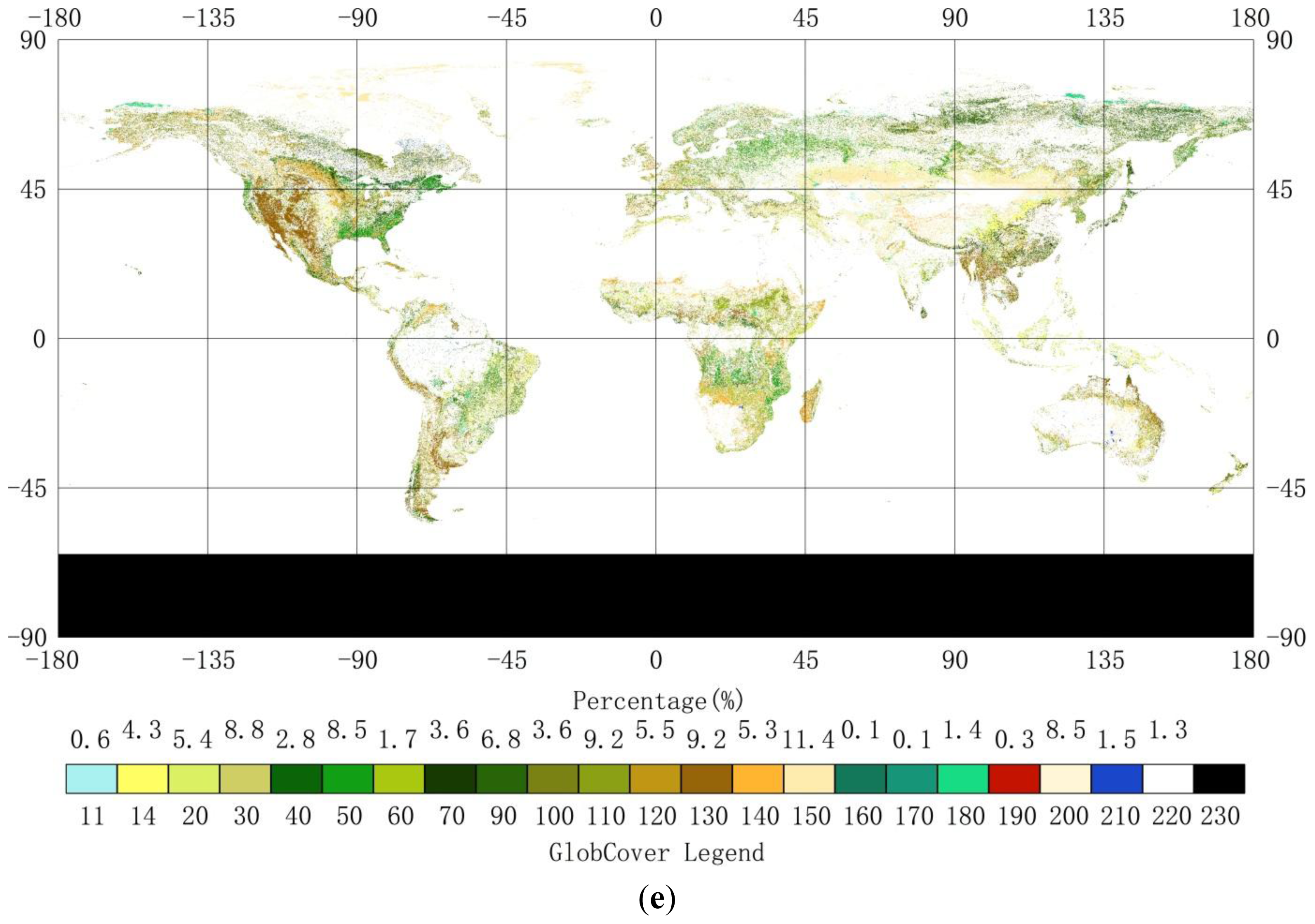
2.1. Land-Cover Datasets

Five global land cover datasets were used in this study, which are GLCC, UMDLC, GLC2000, MCD12Q1 version 051 for year 2005 and GlobCover for year 2009. GLCC was published in various classification legends, one of which with International Geosphere Biosphere Programme (IGBP) land cover classification was chosen in this study. UMDLC was developed with a 14-class labeling and shading schemes. GLC2000 uses the Food and Agriculture Organization (FAO) Land Cover Classification System (LCCS). MCD12Q1 is provided with five global land cover classification systems, among which IGBP legend was selected in this study. The GlobCover was associated with a legend defined and documented using the United Nations (UN) LCCS.

These five land cover data-sets have different spatial resolutions and coverage years as shown in Table 1. How inconsistent classifications and spatial resolutions are harmonized will be described in Section 3.1. Even though some outdated maps were included, their aberrant classifications were recognized and valuable information was considered in our method. The different acquisition dates cannot account for the discrepancy among land cover maps, because land cover change cannot be detected due to insufficient accuracy of the individual land cover maps [23]. We therefore ignored the impacts of land cover changes when designing our fusion method.

2.2. Validation Data

Validation data used in this study (

Table 2. Validation reference data used in this study.

Validation Data	Legend	Sample Size
GLC2000ref	FAO LCCS	1253
GlobCover2005ref	UN LCCS	4258
STEP	IGBP	1780
VIIRS	IGBP	3667

) were acquired from the Global Observation of Forest and Land Cover Dynamics (GOFC-GOLD) Land Cover Project Office in coordination with reference data producers, including consolidated GLC 2000 reference (GLC200ref) dataset [12], consolidated GlobCover 2005 reference (GlobCover2005ref) dataset [26,27], System for Terrestrial Ecosystem Parameterization (STEP) reference dataset [14,15,28–32] and Visible Infrared Imaging Radiometer Suite (VIIRS) Surface Type reference dataset [33,34].

GLC2000ref is the result of a consolidation work realized on the original GLC 2000 dataset with 1253 samples provided [12]. GlobCover-2005ref dataset is the result of a consolidation work realized on the original ESA-GlobCover 2005 dataset; it contains 4258 samples, globally distributed and selected according to a random stratified sampling [26,27]. STEP is maintained as a database of training polygons drawn on high spatial resolution imagery that can be extracted with GIS to produce a global land cover classification, which is the training site database of MCD12Q1 [14,15,28–32]. VIIRS Surface Type validation database is based on a stratified random sample of 500 blocks (5 × 5 km) globally [14,15,28–32]. The correct class of each sample according to the IGBP legend was identified by manual interpretation of very-high spatial resolution (<2 m) image; MODIS time series data were used to improve the interpretations.

3. Method

In this section, we describe our methodology for fusion of five land cover data-sets. The main steps of fusion procedure are represented in the following flowchart (Figure 1).

We first resampled and reclassified each land cover dataset into the same legend and spatial resolution (1/120 degree), denoted by b_k,x,y. We then combined them into a prior global land cover (a_x,y). The pixels with high consistence were then extracted and denoted by C_x,y. Finally, we updated the probability distribution of each pixel ( ${\mathit{a}}_{\text{x},\text{y}}^u$) using Bayes theory and got the posterior global land cover map ( $C_{x,y}^T$).

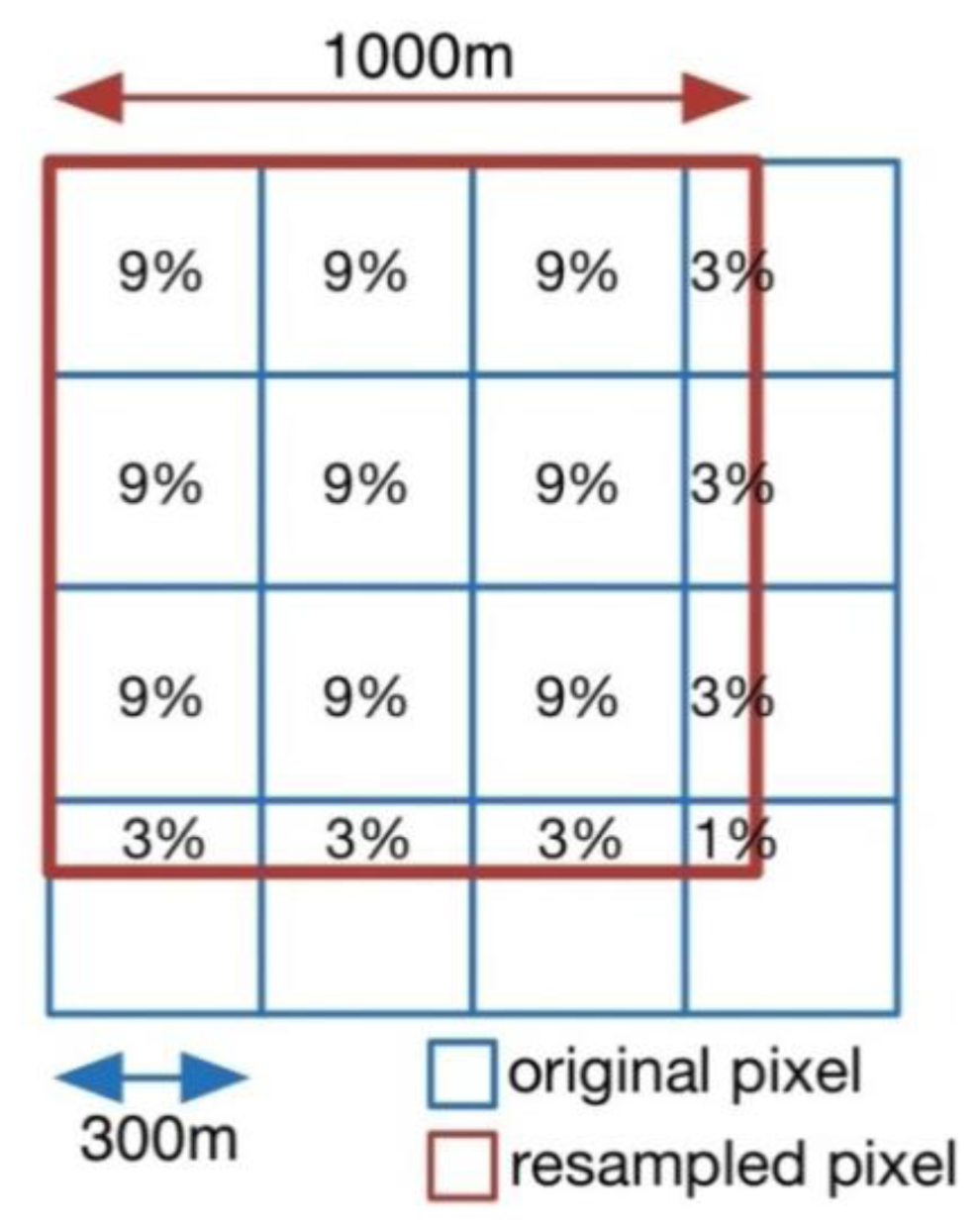
3.1. Reclassification and Resampling

To facilitate fusion of different land cover maps, they need to be homogenized into a common legend, and in this study we selected the IGBP classification system (

Table 3. Numbers and descriptions of International Geosphere Biosphere Programme (IGBP) land cover classification.

IGBP No.	Description
0	Water
1	Evergreen Needleleaf Forest
2	Evergreen Broadleaf Forest
3	Deciduous Needleleaf Forest
4	Deciduous Broadleaf Forest
5	Mixed Forests
6	Closed Shrublands
7	Open Shrublands
8	Woody Savannas
9	Savannas
10	Grasslands
11	Permanent Wetlands
12	Croplands
13	Urban and Built-Up
14	Cropland/Natural Vegetation mosaic
15	Snow and Ice
16	Barren or Sparsely Vegetated

). The 17 categories of IGBP land cover legend embrace the climate independence and canopy component philosophy presented by Running et al. [35], and are compatible with classification systems for environmental modeling for providing landscape information [10]. The correspondence between the IGBP and other legends is rarely 100% [24] and some classes have partial overlap [19]. Simple conversion can produce errors. Thus, in this study every land cover type was translated to a state probability vector representing the probability it belongs to each IGBP land cover type. The state probability vector makes it possible to convert one land cover type to more than one IGBP land cover types and reduce error caused by land cover legend conversion.

Different land cover legends (UMD (

Table 4. Conversion rules from University of Maryland (UMD) land cover legend to International Geosphere Biosphere Programme (IGBP) legend and corresponding state probability vectors. Please see Table 3 for description of IGBP values.

Value	UMD Land Cover Name	IGBP Class Value	State Probability Vector Of IGPB Class (Zero before Decimal Point Omitted)
			0	1	2	3	4	5	6	7	8	9	10	11	12	13	14	15	16
0	Water	0	0.500	0.031	0.031	0.031	0.031	0.031	0.031	0.031	0.031	0.031	0.031	0.031	0.031	0.031	0.031	0.031	0.031
1	Evergreen Needleleaf Forest	1	0.031	0.500	0.031	0.031	0.031	0.031	0.031	0.031	0.031	0.031	0.031	0.031	0.031	0.031	0.031	0.031	0.031
2	Evergreen Broadleaf Forest	2	0.031	0.031	0.500	0.031	0.031	0.031	0.031	0.031	0.031	0.031	0.031	0.031	0.031	0.031	0.031	0.031	0.031
3	Deciduous Needleleaf Forest	3	0.031	0.031	0.031	0.500	0.031	0.031	0.031	0.031	0.031	0.031	0.031	0.031	0.031	0.031	0.031	0.031	0.031
4	Deciduous Broadleaf Forest	4	0.031	0.031	0.031	0.031	0.500	0.031	0.031	0.031	0.031	0.031	0.031	0.031	0.031	0.031	0.031	0.031	0.031
5	Mixed Forests	5	0.031	0.031	0.031	0.031	0.031	0.500	0.031	0.031	0.031	0.031	0.031	0.031	0.031	0.031	0.031	0.031	0.031
6	Woodland	8,11	0.033	0.033	0.033	0.033	0.033	0.033	0.033	0.033	0.250	0.033	0.033	0.250	0.033	0.033	0.033	0.033	0.033
7	Wooded Grassland	9,11	0.033	0.033	0.033	0.033	0.033	0.033	0.033	0.033	0.033	0.250	0.033	0.250	0.033	0.033	0.033	0.033	0.033
8	Closed Shrubland	6	0.031	0.031	0.031	0.031	0.031	0.031	0.500	0.031	0.031	0.031	0.031	0.031	0.031	0.031	0.031	0.031	0.031
9	Open Shrubland	7	0.031	0.031	0.031	0.031	0.031	0.031	0.031	0.500	0.031	0.031	0.031	0.031	0.031	0.031	0.031	0.031	0.031
10	Grassland	10	0.031	0.031	0.031	0.031	0.031	0.031	0.031	0.031	0.031	0.031	0.500	0.031	0.031	0.031	0.031	0.031	0.031
11	Cropland	12,14	0.033	0.033	0.033	0.033	0.033	0.033	0.033	0.033	0.033	0.033	0.033	0.033	0.250	0.033	0.250	0.033	0.033
12	Bare ground	15,16	0.033	0.033	0.033	0.033	0.033	0.033	0.033	0.033	0.033	0.033	0.033	0.033	0.033	0.033	0.033	0.250	0.250
13	Urban and Built-up	13	0.031	0.031	0.031	0.031	0.031	0.031	0.031	0.031	0.031	0.031	0.031	0.031	0.031	0.500	0.031	0.031	0.031
255	No data	-	0.059	0.059	0.059	0.059	0.059	0.059	0.059	0.059	0.059	0.059	0.059	0.059	0.059	0.059	0.059	0.059	0.059

), FAO LCCS (

Table 5. Conversion rules from GLC2000 land cover legend to International Geosphere Biosphere Programme (IGBP) legend and corresponding state probability vectors.

Value	GLC2000-Class	IGBP-Value	State Probability Vector of IGPB Class (Zero before Decimal Point Omitted)
			0	1	2	3	4	5	6	7	8	9	10	11	12	13	14	15	16
1	Tree Cover, broadleaved, evergreen	2	0.031	0.031	0.500	0.031	0.031	0.031	0.031	0.031	0.031	0.031	0.031	0.031	0.031	0.031	0.031	0.031	0.031
2	Tree Cover, broadleaved, deciduous, closed	4	0.031	0.031	0.031	0.031	0.500	0.031	0.031	0.031	0.031	0.031	0.031	0.031	0.031	0.031	0.031	0.031	0.031
3	Tree Cover, broadleaved, deciduous, open	8,9	0.033	0.033	0.033	0.033	0.033	0.033	0.033	0.033	0.250	0.250	0.033	0.033	0.033	0.033	0.033	0.033	0.033
4	Tree Cover, needle-leaved, evergreen	1	0.031	0.500	0.031	0.031	0.031	0.031	0.031	0.031	0.031	0.031	0.031	0.031	0.031	0.031	0.031	0.031	0.031
5	Tree Cover, needle-leaved, deciduous	3	0.031	0.031	0.031	0.500	0.031	0.031	0.031	0.031	0.031	0.031	0.031	0.031	0.031	0.031	0.031	0.031	0.031
6	Tree Cover, mixed leaf type	5	0.031	0.031	0.031	0.031	0.031	0.500	0.031	0.031	0.031	0.031	0.031	0.031	0.031	0.031	0.031	0.031	0.031
7	Tree Cover, regularly flooded, fresh	2,11	0.033	0.033	0.250	0.033	0.033	0.033	0.033	0.033	0.033	0.033	0.033	0.250	0.033	0.033	0.033	0.033	0.033
8	Tree Cover, regularly flooded, saline, (daily variation)	2,11,0	0.167	0.036	0.167	0.036	0.036	0.036	0.036	0.036	0.036	0.036	0.036	.167	0.036	0.036	0.036	0.036	0.036
9	Mosaic: Tree cover/Other natural vegetation	6,7	0.033	0.033	0.033	0.033	0.033	0.033	0.250	0.250	0.033	0.033	0.033	0.033	0.033	0.033	0.033	0.033	0.033
10	Tree Cover, burnt	3,5,7	0.036	0.036	0.036	0.167	0.036	0.167	0.036	0.167	0.036	0.036	0.036	0.036	0.036	0.036	0.036	0.036	0.036
11	Shrub Cover, closed-open, evergreen (with or without sparse tree layer)	7,8	0.033	0.033	0.033	0.033	0.033	0.033	0.033	0.250	0.250	0.033	0.033	0.033	0.033	0.033	0.033	0.033	0.033
12	Shrub Cover, closed-open, deciduous (with or without sparse tree layer)	6,7,9	0.036	0.036	0.036	0.036	0.036	0.036	0.167	0.167	0.036	0.167	0.036	0.036	0.036	0.036	0.036	0.036	0.036
13	Herbaceous Cover, closed-open	6,10	0.033	0.033	0.033	0.033	0.033	0.033	0.250	0.033	0.033	0.033	0.250	0.033	0.033	0.033	0.033	0.033	0.033
14	Sparse Herbaceous or sparse shrub cover	7,10	0.033	0.033	0.033	0.033	0.033	0.033	0.033	0.250	0.033	0.033	0.250	0.033	0.033	0.033	0.033	0.033	0.033
15	Regularly flooded shrub and/or herbaceous cover	7,11	0.033	0.033	0.033	0.033	0.033	0.033	0.033	0.250	0.033	0.033	0.033	0.250	0.033	0.033	0.033	0.033	0.033
16	Cultivated and managed areas	12	0.031	0.031	0.031	0.031	0.031	0.031	0.031	0.031	0.031	0.031	0.031	0.031	0.500	0.031	0.031	0.031	0.031
17	Mosaic: Cropland/Tree Cover/Other Natural Vegetation	14	0.031	0.031	0.031	0.031	0.031	0.031	0.031	0.031	0.031	0.031	0.031	0.031	0.031	0.031	0.500	0.031	0.031
18	Mosaic: Cropland/Shrub and/or Herbaceous cover	14	0.031	0.031	0.031	0.031	0.031	0.031	0.031	0.031	0.031	0.031	0.031	0.031	0.031	0.031	0.500	0.031	0.031
19	Bare Areas	16	0.031	0.031	0.031	0.031	0.031	0.031	0.031	0.031	0.031	0.031	0.031	0.031	0.031	0.031	0.031	0.031	0.500
20	Water Bodies (natural & artificial)	0	0.500	0.031	0.031	0.031	0.031	0.031	0.031	0.031	0.031	0.031	0.031	0.031	0.031	0.031	0.031	0.031	0.031
21	Snow and Ice (natural & artificial)	15	0.031	0.031	0.031	0.031	0.031	0.031	0.031	0.031	0.031	0.031	0.031	0.031	0.031	0.031	0.031	0.500	0.031
22	Artificial surfaces and associated areas	13	0.031	0.031	0.031	0.031	0.031	0.031	0.031	0.031	0.031	0.031	0.031	0.031	0.031	0.500	0.031	0.031	0.031
23	No data	-	0.059	0.059	0.059	0.059	0.059	0.059	0.059	0.059	0.059	0.059	0.059	0.059	0.059	0.059	0.059	0.059	0.059

) and UN LCCS (

Table 6. Conversion rules from GlobCover land cover legend to International Geosphere Biosphere Programme (IGBP) legend and corresponding state probability vectors.

Value	GlobCover-Label	IGBP Value	State Probability Vector of IGPB Class (Zero before Decimal Point Omitted)
			0	1	2	3	4	5	6	7	8	9	10	11	12	13	14	15	16
11	Post-flooding or irrigated croplands (or aquatic)	12	0.031	0.031	0.031	0.031	0.031	0.031	0.031	0.031	0.031	0.031	0.031	0.031	0.500	0.031	0.031	0.031	0.031
14	Rainfed croplands	12	0.031	0.031	0.031	0.031	0.031	0.031	0.031	0.031	0.031	0.031	0.031	0.031	0.500	0.031	0.031	0.031	0.031
20	Mosaic cropland (50%–70%)/vegetation (grassland/shrubland/forest) (20%–50%)	12,14	0.033	0.033	0.033	0.033	0.033	0.033	0.033	0.033	0.033	0.033	0.033	0.033	0.250	0.033	0.250	0.033	0.033
30	Mosaic vegetation (grassland/shrubland/forest) (50%–70%)/cropland (20%–50%)	10,14	0.033	0.033	0.033	0.033	0.033	0.033	0.033	0.033	0.033	0.033	0.250	0.033	0.033	0.033	0.250	0.033	0.033
40	Closed to open (>15%) broadleaved evergreen or semi-deciduous forest (>5 m)	2	0.031	0.031	0.500	0.031	0.031	0.031	0.031	0.031	0.031	0.031	0.031	0.031	0.031	0.031	0.031	0.031	0.031
50	Closed (>40%) broadleaved deciduous forest (>5 m)	4	0.031	0.031	0.031	0.031	0.500	0.031	0.031	0.031	0.031	0.031	0.031	0.031	0.031	0.031	0.031	0.031	0.031
60	Open (15%–40%) broadleaved deciduous forest/woodland (>5 m)	8	0.031	0.031	0.031	0.031	0.031	0.031	0.031	0.031	0.500	0.031	0.031	0.031	0.031	0.031	0.031	0.031	0.031
70	Closed (>40%) needleleaved evergreen forest (>5 m)	1,6	0.033	0.250	0.033	0.033	0.033	0.033	0.250	0.033	0.033	0.033	0.033	0.033	0.033	0.033	0.033	0.033	0.033
90	Open (15%–40%) needleleaved deciduous or evergreen forest (>5 m)	1,3,5,8	0.038	0.125	0.038	0.125	0.038	0.125	0.038	0.038	0.125	0.038	0.038	0.038	0.038	0.038	0.038	0.038	0.038
100	Closed to open (>15%) mixed broadleaved and needleleaved forest (>5 m)	5	0.031	0.031	0.031	0.031	0.031	0.500	0.031	0.031	0.031	0.031	0.031	0.031	0.031	0.031	0.031	0.031	0.031
110	Mosaic forest or shrubland (50%–70%)/grassland (20%–50%)	6	0.031	0.031	0.031	0.031	0.031	0.031	0.500	0.031	0.031	0.031	0.031	0.031	0.031	0.031	0.031	0.031	0.031
120	Mosaic grassland (50%–70%)/forest or shrubland (20%–50%)	7	0.031	0.031	0.031	0.031	0.031	0.031	0.031	0.500	0.031	0.031	0.031	0.031	0.031	0.031	0.031	0.031	0.031
130	Closed to open (>15%) (broadleaved or needleleaved, evergreen or deciduous) shrubland (<5 m)	6,9	0.033	0.033	0.033	0.033	0.033	0.033	0.250	0.033	0.033	0.250	0.033	0.033	0.033	0.033	0.033	0.033	0.033
140	Closed to open (>15%) herbaceous vegetation (grassland, savannas or lichens/mosses)	7,10	0.033	0.033	0.033	0.033	0.033	0.033	0.033	0.250	0.033	0.033	0.250	0.033	0.033	0.033	0.033	0.033	0.033
150	Sparse (<15%) vegetation	7,16	0.033	0.033	0.033	0.033	0.033	0.033	0.033	0.250	0.033	0.033	0.033	0.033	0.033	0.033	0.033	0.033	0.250
160	Closed to open (>15%) broadleaved forest regularly flooded (semi-permanently or temporarily)-Fresh or brackish water	2	0.031	0.031	0.500	0.031	0.031	0.031	0.031	0.031	0.031	0.031	0.031	0.031	0.031	0.031	0.031	0.031	0.031
170	Closed (>40%) broadleaved forest or shrubland permanently flooded-Saline or brackish water	11	0.031	0.031	0.031	0.031	0.031	0.031	0.031	0.031	0.031	0.031	0.031	0.500	0.031	0.031	0.031	0.031	0.031
180	Closed to open (>15%) grassland or woody vegetation on regularly flooded or waterlogged soil-Fresh, brackish or saline water	11	0.031	0.031	0.031	0.031	0.031	0.031	0.031	0.031	0.031	0.031	0.031	0.500	0.031	0.031	0.031	0.031	0.031
190	Artificial surfaces and associated areas (Urban areas >50%)	13	0.031	0.031	0.031	0.031	0.031	0.031	0.031	0.031	0.031	0.031	0.031	0.031	0.031	0.500	0.031	0.031	0.031
200	Bare areas	16	0.031	0.031	0.031	0.031	0.031	0.031	0.031	0.031	0.031	0.031	0.031	0.031	0.031	0.031	0.031	0.031	0.500
210	Water bodies	0,15	0.250	0.033	0.033	0.033	0.033	0.033	0.033	0.033	0.033	0.033	0.033	0.033	0.033	0.033	0.033	0.250	0.033
220	Permanent snow and ice	15	0.031	0.031	0.031	0.031	0.031	0.031	0.031	0.031	0.031	0.031	0.031	0.031	0.031	0.031	0.031	0.500	0.031
230	No data (burnt areas, clouds, …)	-	0.059	0.059	0.059	0.059	0.059	0.059	0.059	0.059	0.059	0.059	0.059	0.059	0.059	0.059	0.059	0.059	0.059

)) were converted to the IGBP legend according to comparison of legend definitions, pixel-by-pixel statistical comparison and previous comparison studies [36–38]. Because of insufficient information, each land cover type was converted to several IGBP land cover types equi-probably. Considering possible classification mistakes, we assumed that each pixel of every land cover map was classified into a wrong class with 50% probability. That is to say, in state probability vector of a certain land cover class, the total probability for all specified IGBP classes is 50%. This assumption will not substantially change the classification of each pixel but will allow for assessing the uncertainties of classification of land cover maps.

All the global land cover maps need to be projected to the same projection (geographical projection in this study) and resampled to the same spatial resolution (1/120 geographical degree in this study). The state vector of each resampled pixel was the average of original pixels’ state vectors, weighted by their area overlapped with resampled pixel. For example, when resampling from 300 m to 1 km, which does not fit with each other, as shown in Figure 2, land cover state probability vectors of resampled pixels were combined based on the overlapped area with original pixels. By this method, no information will be lost when resampling.

Finally, all the global land cover data-sets were homogenized. The state probability vector of pixel located in the x-th path of y-th line in k-th land cover map is represented by b_k,x,y, of which b_k,x,y(i) stands for the probability it belongs to the i-th IGBP class.

3.2. Generate Prior Global Land Cover Map

A prior global land cover needed by the Bayes method was generated by aggregating information provided by the existing land cover products, in which the prior state probability vector of pixel (x, y) is denoted by a_x,y. Therefore, we need to combine probability distributions b_k,x,y in existing land cover products into one. Without any other information available, simple axiomatic approaches [39] were used, such as linear opinion pool,

$${\mathit{a}}_{\text{x},\text{y}}=\frac{{\sum }_{k=1}^N{w}_k{\mathit{b}}_{\mathbf{k},\mathbf{x},\mathbf{y}}}{{\sum }_{k=1}^N{w}_k}$$

(1)

and logarithmic opinion pool

$${\mathit{a}}_{\text{x},\text{y}}=\beta \hspace{0.17em}\left(\prod _{k=1}^N{{\mathit{b}}_{\text{k},\text{x},\text{y}}}^{w_k}\right)$$

(2)

where N is the number of land cover maps used (N = 5 in this study). w_k is the weight of the k-th land cover map (w_k = 1 in this study). β is normalizing constant. The prior land cover class is denoted by C_x,y, which was derived from

$${\mathit{a}}_{\text{x},\text{y}}(C_{\mathbf{x},\mathbf{y}})=\underset{0\le i\le M}{\text{max}}{\mathit{a}}_{\text{x},\text{y}}(i)$$

(3)

where M is the number of classes in the common legend (M = 17 for IGBP legend in this study). The parameter a_x,y(C_x,y) represents classification certainty for pixel (x, y). Without further information about which method is more accurate, both linear and logarithmic opinion pools were used when generating prior global land cover map in this study and their differences were also compared.

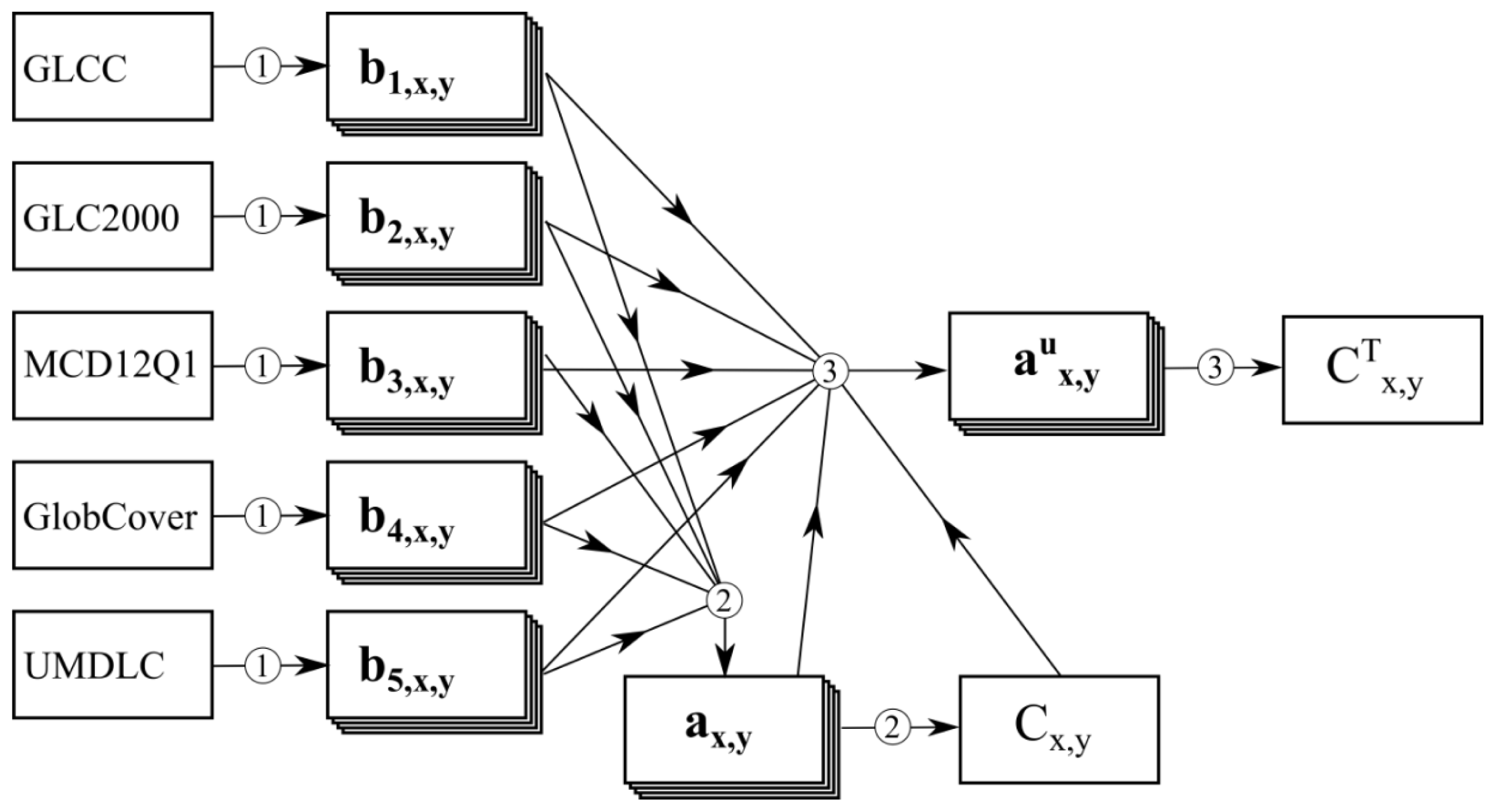
3.3. Update State Vector of Each Pixel

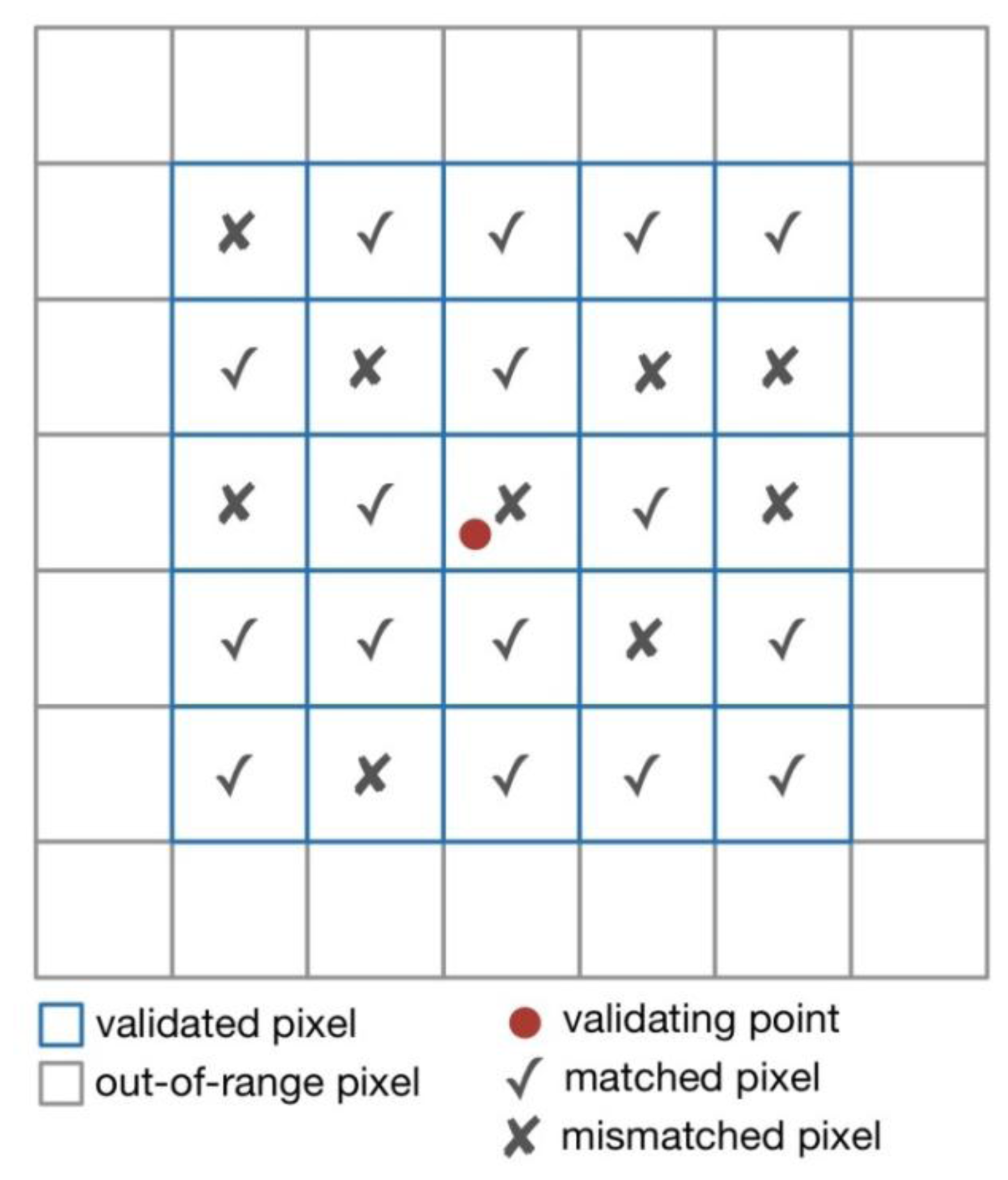
The state probability vector of each pixel in the prior global land cover map was updated based on Bayes theorem. The updated probability for pixel (x, y) can be written as conditional probability given classifications of existing land cover products:

$${\mathit{a}}_{\text{x},\text{y}}^u(t)=P(C_{x,y}^T=t\mid \underset{k=1}{\overset{N}{\cap }}{C}_{\text{k},\text{x},\text{y}})$$

(4)

where $C_{x,y}^T$ is the true class of pixel (x, y), which is unknown, and t = 0,1,2, …, M − 1. The symbol ∩ denotes joint probability, C_k,x,y denotes the maximum likelihood land cover class in the state probability vector of pixel (x, y) in the k-th land cover map, which means b_k,x,y(C_k,x,y) = max_0≤i<M b_k,x,y(i). According to Bayes formula, above conditional probability can be written as:

$${\mathit{a}}_{\text{x},\text{y}}^u(t)=\alpha P\hspace{0.17em}\left(\underset{k=1}{\overset{N}{\cap }}{C}_{\text{k},\text{x},\text{y}}|C_{x,y}^T=t\right)\hspace{0.17em}P(C_{x,y}^T=t)$$

(5)

where α is a normalizing constant. $P(C_{x,y}^T=t)$ is the prior probability that true class of pixel (x, y) is t and identical to a_x,y(t). Given the assumption that each land cover map is independent, Equation (5) can be rewritten as

$${\mathit{a}}_{\text{x},\text{y}}^u(t)=\alpha \prod _{k=1}^{N}P(C_{\text{k},\text{x},\text{y}}\mid C_{x,y}^T=t)\hspace{0.17em}{\mathit{a}}_{\text{x},\text{y}}(t)$$

(6)

Here, $\alpha {\prod }_{k=1}^{N}P({\mathit{b}}_{k,x,y}\mid C_{x,y}^T=t)$ is the updating coefficient of prior state vector a_x,y(t).

For any k = 1,2, …, N in the updating coefficient, we have

$$P(C_{\text{k},\text{x},\text{y}}\mid C_{x,y}^T=t)=\frac{P(C_{\text{k},\text{x},\text{y}}\cap C_{x,y}^T=t)}{P(C_{x,y}^T=t)}$$

(7)

As we do not know the true class $C_{x,y}^T$ for any pixel (x, y), we assume that for any pixel (x, y) $C_{x,y}^T=C_{\text{x},\text{y}}$ if its certainty a_x,y(C_x,y) is higher than a given threshold. This threshold varies for different classes and is defined as the upper quartile of certainties for each class, so we have:

$$P(C_{\text{k},\text{x},\text{y}}\mid C_{x,y}^T=t)=\frac{{\sum }_{\mathit{x},\mathit{y}}{\mathit{b}}_{k,x,y}(C_{\text{k},\text{x},\text{y}})}{{\sum }_{\mathit{x},\mathit{y}}1}{\mid }_{C_{\mathbf{x},\mathbf{y}}=t,{\mathit{a}}_{\text{x},\text{y}}(C_{\mathbf{x},\mathbf{y}})<h_t}$$

(8)

where h_t is the certainty threshold for class t. In other words, we figured out the probability in Equation (8) by summarizing under condition of C_x,y = t and a_x,y(C_x,y) > h_t.

After substituting Equation (8) into Equation (5) and normalization, we obtained the updated state vector ${\mathit{a}}_{\text{x},\text{y}}^u$. Furthermore, the posterior global land cover map $C_{x,y}^p$ was derived from:

$${\mathit{a}}_{\text{x},\text{y}}^u(C_{x,y}^p)=\underset{0\le i\le M}{\text{max}}\hspace{0.17em}{\mathit{a}}_{\text{x},\text{y}}^u(i)$$

(9)

3.4. Validation

Four validation data-sets have different land cover classifications (Table 2). When validating, comparisons between land cover legends of validation data-sets and land cover map need to be defined. We regarded the two land cover types from different legends as identical if they can be translated to the same IGBP classes according to the conversion rules defined above (Tables 4–6). For example, type 13 of GLC2000 legend was converted to types 6 and 10 of IGBP legend (Table 5), and type 140 of GlobCover legend was converted to types 7 and 10 of IGBP legend (Table 6); then we took GLC2000 class 13 and GlobCover class 140 as identical when validating GlobCover with GLC2000ref.

Considering the spatial representativeness, geo-location errors and pixel-shift errors of validation points, every validation point was compared with the pixel it located at and its 2-order neighboring pixels. The percentage of matched pixels was defined as validation accuracy. An example is shown in Figure 3. The total validation accuracy of a land cover map was defined as average accuracy of all the validating points in a reference data-set.

4. Result

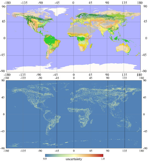
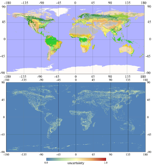
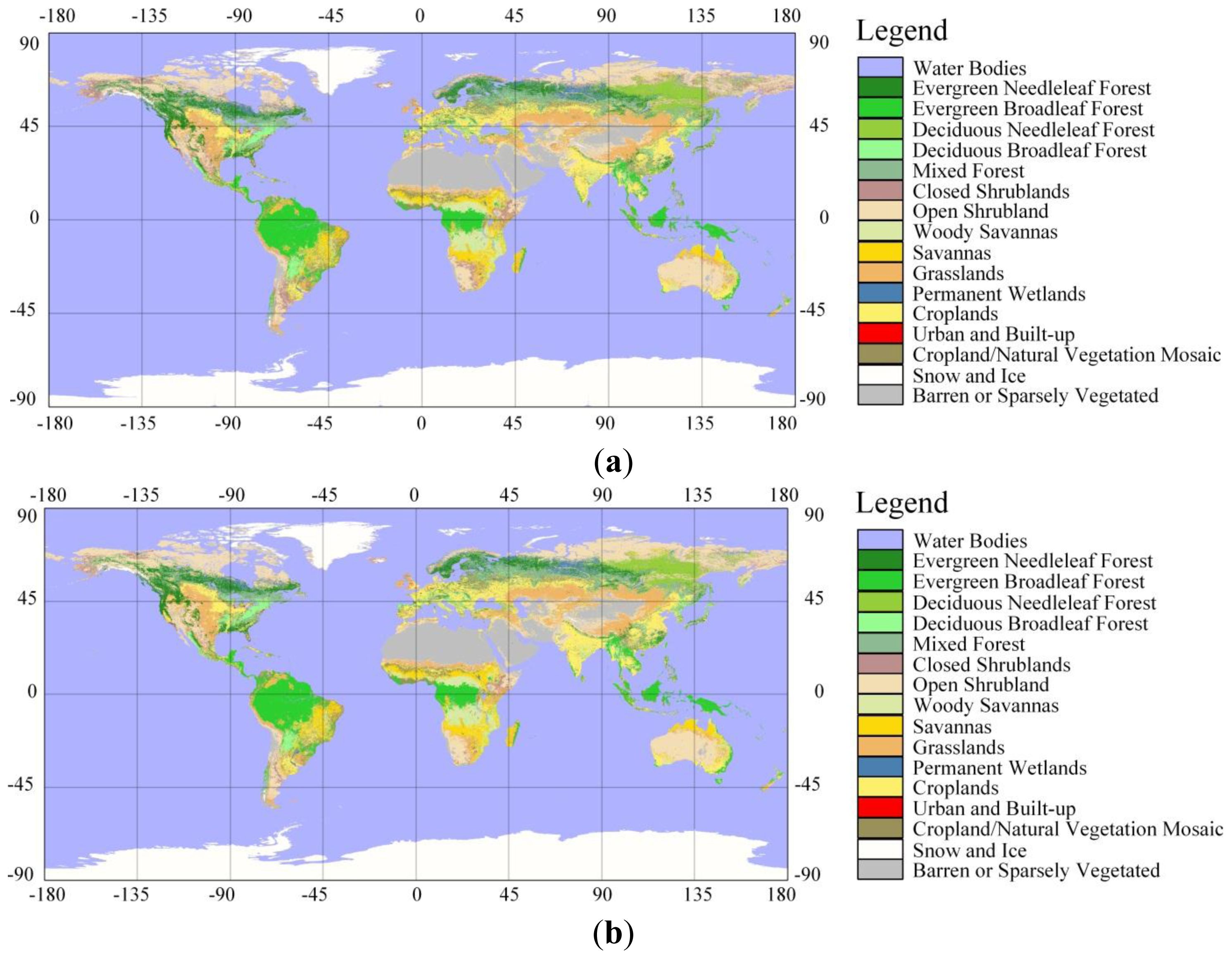
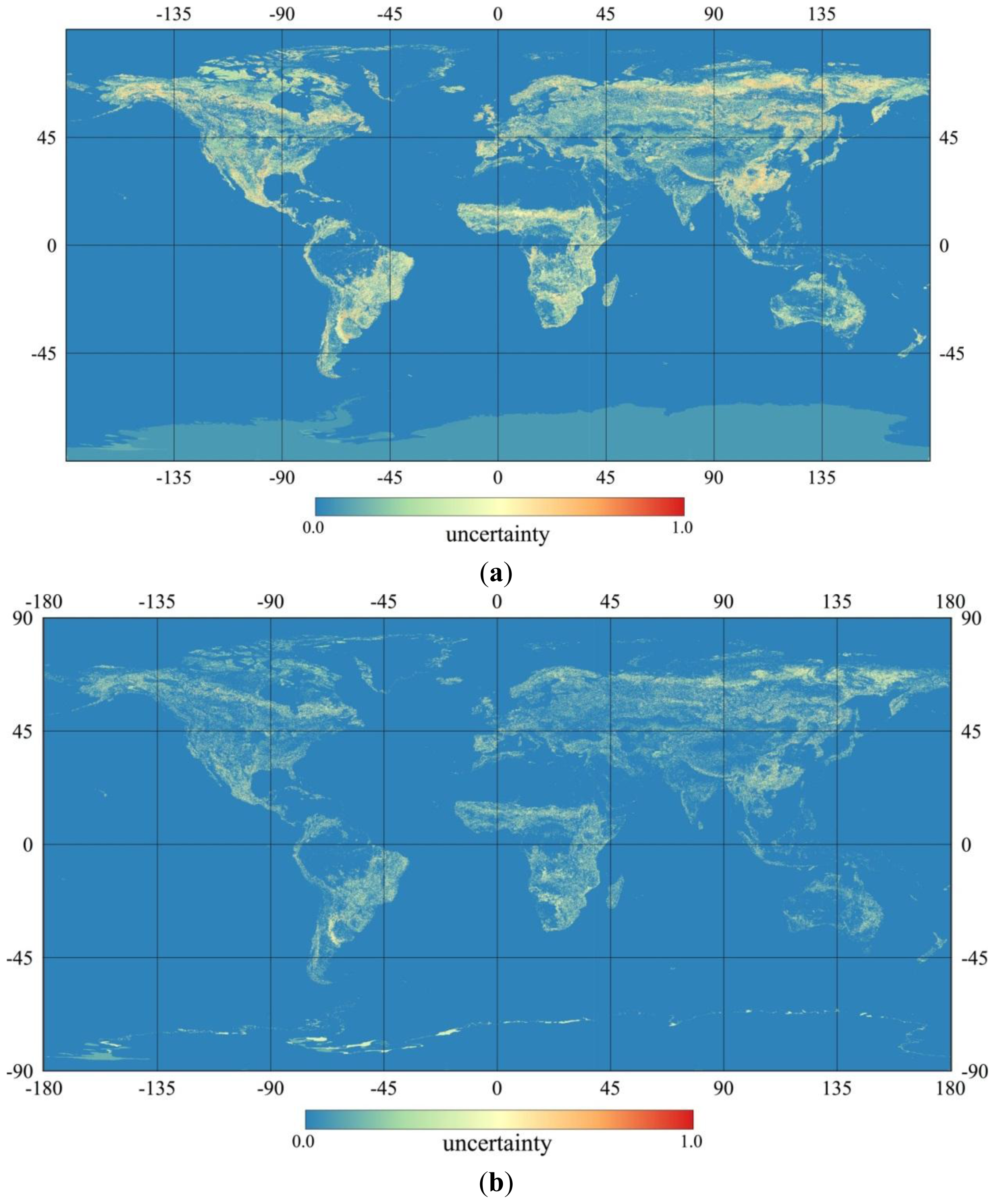
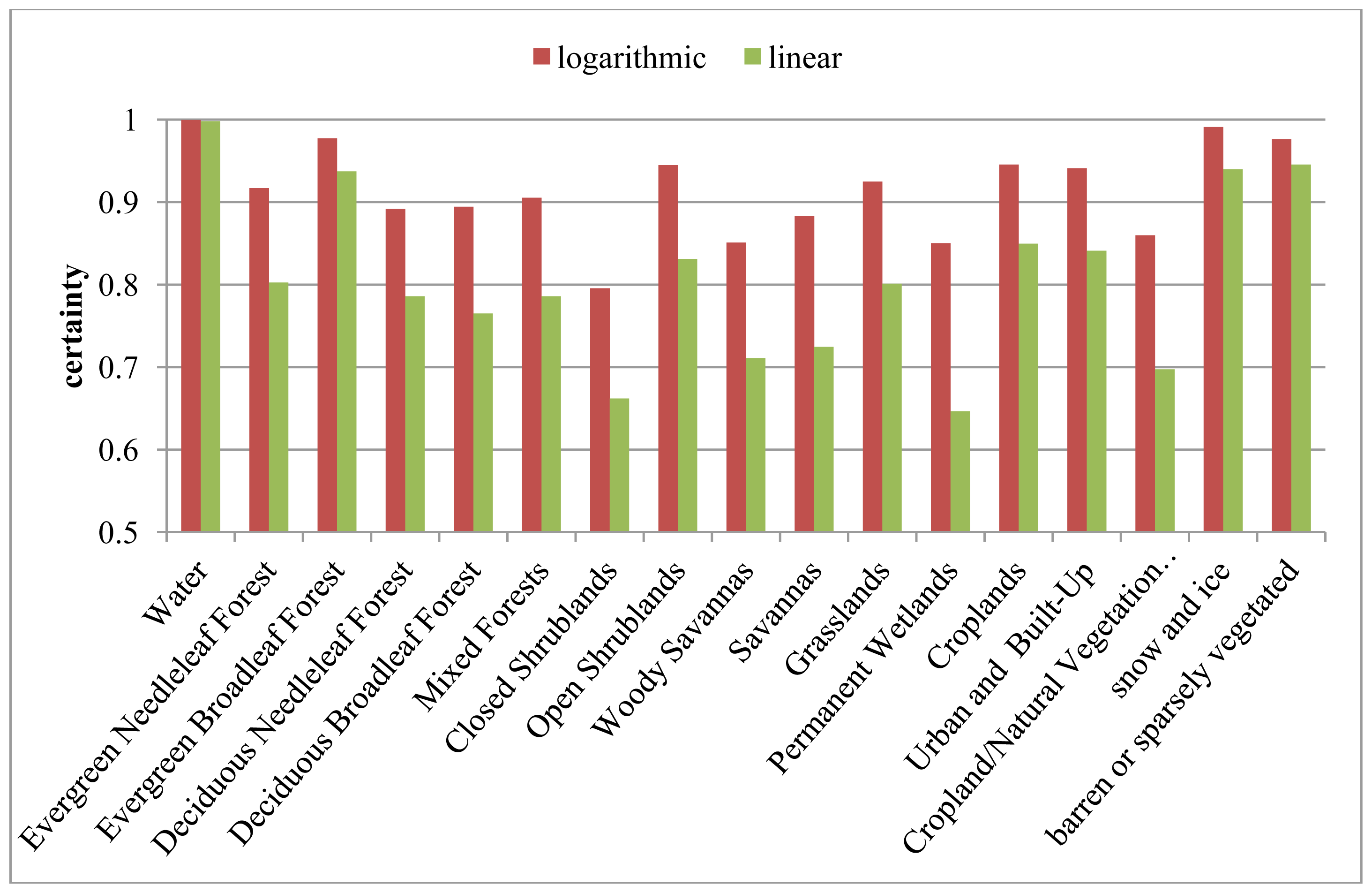
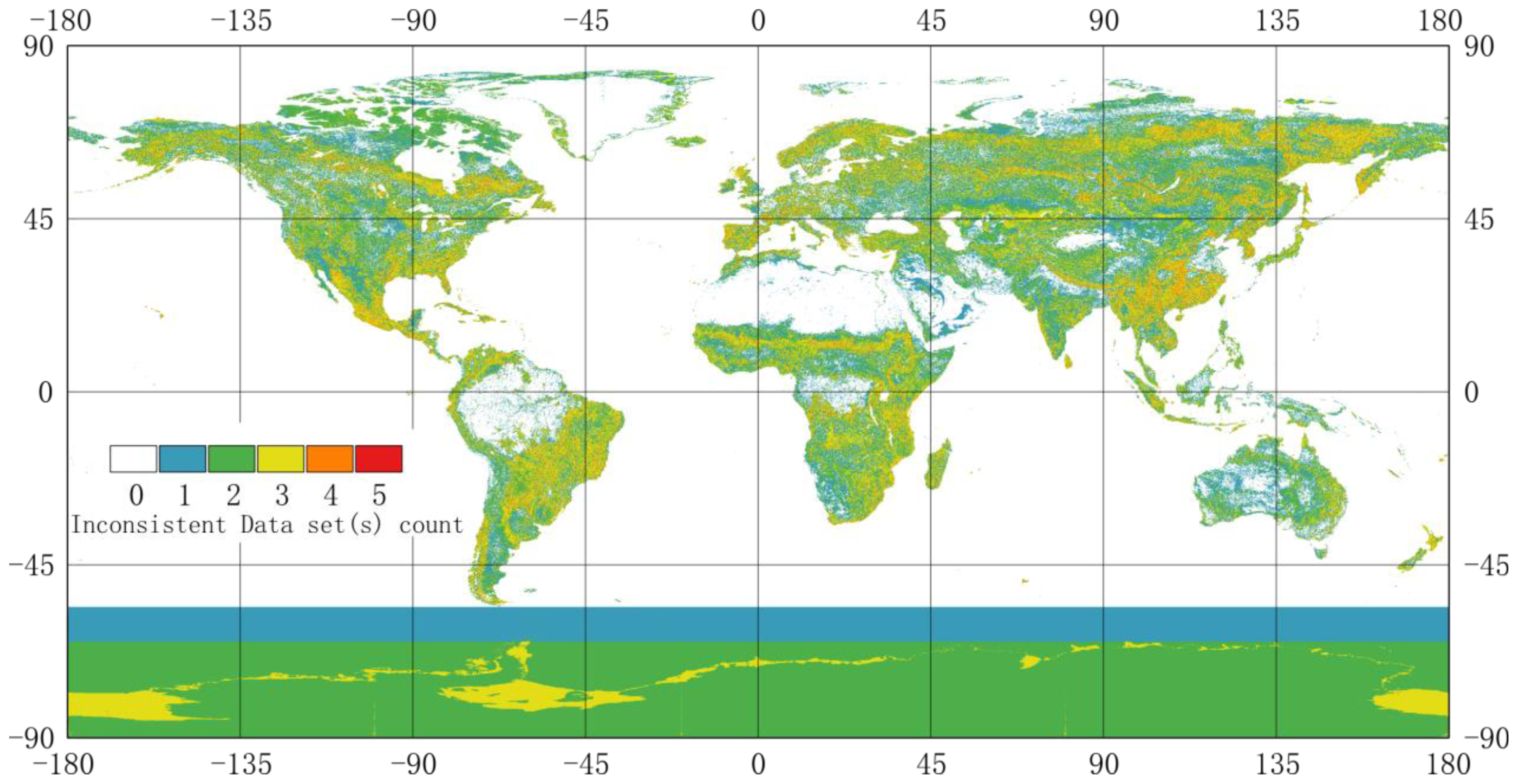
4.1. Posterior Global Land Cover Map and its Uncertainty

Using the method proposed in this study, a synergetic global land cover (synGLC-linear and synGLC-log) dataset ( $C_{x,y}^p$) with an additional information on their certainties ( ${\mathit{a}}_{\mathbf{x},\mathbf{y}}^{\mathit{u}}(C_{x,y}^p)$, the maximum of state probability vector) was generated (Figures 4 and 5) based on prior land cover maps from linear (Equation (1)) and logarithmic (Equation (2)) opinion pool. The most conspicuous differences between these two posterior maps were found in the Antarctic, which was probably due to the uncertainty caused by melting ice sheet during the past decades. Spatial patterns of classification certainties (Figure 5) were similar, and most high uncertain pixels distributed in land cover transition regions. The preferable synGLC map was decided after validation (see Section 4.2).

To understand the differences between these two posterior maps, percentages of each land cover class (represented by number of pixels) are shown in

Table 7. Pixel percentages of each land cover type in the posterior land cover maps.

IGBP	Description	Linear	Logarithmic	Relative Difference
0	Water	67.83%	67.35%	−0.71%
1	Evergreen Needleleaf Forest	1.33%	1.30%	−2.24%
2	Evergreen Broadleaf Forest	1.82%	1.86%	2.11%
3	Deciduous Needleleaf Forest	0.67%	0.66%	−1.92%
4	Deciduous Broadleaf Forest	0.58%	0.56%	−4.07%
5	Mixed Forests	1.18%	1.26%	6.63%
6	Closed Shrublands	1.22%	0.66%	−46.09%
7	Open Shrublands	4.00%	4.42%	10.65%
8	Woody Savannas	1.04%	1.05%	0.96%
9	Savannas	0.98%	1.02%	4.32%
10	Grasslands	1.98%	2.06%	4.05%
11	Permanent Wetlands	0.37%	0.32%	−11.59%
12	Croplands	2.27%	2.45%	7.98%
13	Urban and Built-Up	0.06%	0.06%	0.30%
14	Cropland/Natural Vegetation mosaic	1.32%	1.14%	−13.41%
15	Snow and Ice	10.58%	10.89%	2.92%
16	Barren or Sparsely Vegetated	2.79%	2.95%	5.81%

. Additionally, their average certainties for each land cover are shown in Figure 6. Closed shrublands, open shrublands, cropland/natural vegetation mosaic and permanent wetlands had the most differences between posterior linear and logarithmic land cover maps. Accordingly, these classes had low averaged certainties (Figure 6), indicating high uncertainties existed.

Posterior logarithmic land cover map had higher certainty than the linear one for every class, but it was the result of different calculations and did not imply that the logarithmic one was better. It was different prior land cover maps that engendered differences in posterior uncertainty. The certainty was only comparable within the same prior land cover map in this approach. Validating with other reference data was necessary to assess the performance of our method and decide which land cover map is better.

4.2. Validation

Table 8. Accuracy and corresponding ranking of each land cover map when validated with different reference data.

Reference Data	GlobCover2005ref	GLC2000ref	STEP	VIIRS	Average
Land Cover Maps
synGLC-linear	66.56%/4	57.04%/3	60.88%/3	40.27%/4	56.19%/3.5
synGLC-log	66.8%/3	57.18%/2	62.68%/2	40.89%/3	56.89%/2.5
GLC2000	68.13%/2	61.24%/1	52.74%/4	38.48%/5	55.14%/3.0
GLCC	57.19%/7	49.46%/5	41.42%/7	33.11%/7	45.3%/6.5
GlobCover	70.43%/1	56.55%/4	50.7%/5	41.13%/2	54.7%/3.0
MCD12Q1	63%/5	49.41%/6	85.34%/1	46.28%/1	61.01%/3.25
UMDLC	59.54%/6	43.03%/7	46%/6	36.64%/6	46.3%/6.25

shows the validation results using the method described in Section 3.4. The synGLC-log has higher accuracy than synGLC-linear, thus later we only discuss the synGLC-log (hereafter refer to synGLC).

It is reasonable that every land cover map has the highest accuracy when validating with their own reference data. For example, the GlobCover land cover map ranks first for GlobCover2005ref, and it is the same for the GLC2000ref (GLC2000 reference data). MCD12Q1 ranks first for VIIRS and STEP, because STEP is its training data and VIIRS is interpreted with help of MODIS image. The synGLC ranks second or third in every reference data. Because the synthetic map introduced information from other datasets, it will inevitably decrease the accuracy when validating with their own reference data. However, considering each map has its own bias on its reference or training data, the integrated map is considered to be less biased. The synGLC has the highest average ranking (2.5) followed by GLC2000 (3.0) and GlobCover (3.0), indicating that it has the best overall performance when validating with four reference data sets.

The MCD12Q1 has the highest average accuracy, followed by synGLC, due to its extraordinary high accuracy in STEP and VIIRS. However, it has unfavorable accuracy when validated with GlobCover2005ref and GLC2000ref. In contrast, our synGLC map has fine accuracy when validated with every reference data set, and thus has the best overall performance and is much less biased compared with other products.

4.3. Compare synGLC with the Existing Global Land Cover Maps

To unravel how much information from each land cover product contributes to synGLC, the differences between synGLC and previous land cover products were compared (Figure 7). Classifications that could not be converted to IGBP classifications in synGLC according to the rules (Tables 4–6) are defined as inconsistent.

The fewest inconsistent pixels were found between MCD12Q1 and synGLC (7.73%), and the largest inconsistencies were found in grasslands, open shrublands, woody savannas and cropland/natural vegetation mosaic, which indicated that the synGLC is closest to the dataset with the highest average accuracy (MCD12Q1). GLCC has the second fewest inconsistent pixels with synGLC (8.54%), most of which are mixed forests, cropland/natural vegetation mosaic, open shrub-land, snow and ice. About 9.45% pixels of UMDLC are inconsistent with synGLC, and most of which are woodland, wooded grassland, grassland, closed and open shrub-land. Inconsistency percentages of GLC2000 and GlobCover2009 are relatively higher than others, which are 26.58% and 22.05%, respectively, mainly because of their insufficient information within Antarctica. For GLC2000, most of the inconsistent pixels are herbaceous cover (closed-open), cultivated and managed areas, tree cover. For GlobCover2009, most of the inconsistent pixels were Sparse (<15%) vegetation, mosaic forest or shrub-land (50%–70%)/grassland (20%–50%) and closed to open (>15%, broadleaved or needle-leaved, evergreen or deciduous) shrub-land (<5 m).

For each pixel, the number of land cover maps that have inconsistent classification with synGLC based on Figure 7 is shown in Figure 8. The inconsistency values of more than 90% pixels are equal or less than 2. Most of the consistent pixels (zero inconsistency) are distributed in the ocean, desert regions of North Africa, Amazon rainforests and barren regions. The highly inconsistent pixels are mainly distributed in transition zones, such as tropical forests and savannahs. Because GLC2000 and GlobCover2009 did not provide the land cover map within the Antarctic, the coastline of Antarctica in synGLC comes from the information in UMDLC, GLCC and MCD12Q1.

The percentage of pixels with different inconsistency in each land cover class of synGLC is shown in Figure 9. Water and barren or sparsely vegetated region have the highest consistency. Among the five forest classes, evergreen broadleaf forest has the highest consistency. The pattern of inconsistency among these six global land cover data-sets (five original ones and the synGLC) is similar to that of uncertainty (Figure 6).

5. Discussion

5.1. Assumptions and Limitations

Our fusing method is based on Bayes theory and assumptions that makes the technique practicable. All the assumptions we made are as follows:

(1)

Each land cover map can make a mistake with 50% probability;

(2)

Classification of each land cover map is independent;

(3)

Classification with high agreement is true.

Assumption 1 does not change the information in each land cover map but reduces error of misclassification and legends conversion. Assumption 2 is likely to be true considering each land cover map is produced by different researchers with different data and techniques. It makes it possible to solve the probability equation without thinking about covariance. Assumption 3 helps to construct the benchmark pixels and update the prior probability.

Intuitively, hybrid land cover map should make the most of all the advantages of every land cover product and was expected to have the highest accuracy under any circumstance. However, several limitations still exist and prevent it from achieving its ideal state. The most important limitation is that a wrong prior state probability vector cannot be corrected if all the land cover products have wrong classifications, because we need Assumption 3 to distinguish good or bad classifications. To overcome the bias introduced by this assumption, we can use independent third-party reference data as benchmark to update the prior land cover map and generate a posterior one. This method can definitely be more effective with fewer assumptions.

5.2. Legends Translation

One major problem of our method is subjective definition of land type legend conversion. Any two classes in different legends cannot be identical, and probably have overlapped definitions. Legend homogenization always produces errors. Detailed comparison of different legends is complicated and beyond this research. Consequently, we defined our legends translation rules according to the previous comparison researches [36–38] with some modifications.

First of all, to tackle the legend mismatch problem we defined the state probability vector to make it possible to convert from one class into multiple classes without losing information. Furthermore, we assumed that any land cover product may make mistakes (Assumption 1) to weaken the noise in land cover information. All these techniques can reduce the error cause by legend conversion. However, the rules described by the state probability vector are far from precise. More information is required to make it more accurate—rather than the equi-probable distribution found in this study—which requires that more researches be carried out on the quantitative relationship between different land cover legends.

5.3. Effects of Land Cover Changes

Uncertainties in synGLC mostly come from two sources: land cover changes and inaccuracies of land cover products. How these two factors affect the fusing method and the synGLC is important for understanding the reliability of our method and the accuracy of synGLC. However, due to the lack of sufficient land cover data in long time series, we cannot directly assess the effects of land cover changes.

By simple comparison of GLCC, GLC2000 and MODIS, Jung et al. [23] concluded that land cover change between 1993 and 2000 cannot explain their inconsistencies. In our research, inconsistency percentages among land cover products range from 23% to 30%, excluding area of ocean. Additionally, their accuracies range from 45% (GLCC) to 61% (MCD12Q1). In contrast, the uncertainties stemmed from land cover changes are relatively smaller. For example, only 8.6% of land in the United States experienced changes from 1973 to 2000 [40]. Interannual variations derived from MODIS land cover time series is about 10%, which is higher than actual global land cover change [14].

Given the facts above, we can surmise that the principal source of uncertainties in SynGLC was inaccuracy in land cover classification and the effects of land cover changes are ignorable. Our method mainly focuses on handling inconsistencies among land cover maps and achieving an optimal estimate.

5.4. Strength of Our Method

Although there are so many limitations, a significant advantage of our method is its remarkable extensibility. It can fuse land cover maps with different spatial resolutions and different legends by adjusting the state vector and parameters of resampling accordingly. Even other land surface parameters (such as leaf attributes, LAI) can be integrated if they are related to land cover and can be translated into a state probability vector of land cover classes. This method can synergize the regional land cover maps into the global map by defining the state vector of no data pixel as a uniformly distributed one. In that way, all the available regional land cover maps can be fused into a global one to make use of all available information.

In addition, our method can integrate both old (such as UMDLC) and new (such as GlobCover2009) land cover products and generate the average state of global land cover during the whole time range of input products. It is important for land surface models that are run with a constant land cover parameter. Besides, weight coefficients in Equations (1) and (2) can be modified according to research interests. They directly affect the prior land cover map a_x,y and C_x,y, which will be used to generate a posterior map. Therefore, the different weight coefficients would bring different biases into the synergetic land cover map. Such biases maybe compensate the inaccuracy in land cover products if increasing the weights of land cover maps with high accuracy. In addition, such biases can be used to estimate the land cover map over a certain time span, by increasing the weighting of land cover maps within the time range.

6. Conclusions

In this paper, we demonstrated a technique based on Bayes theory to generate hybrid global land cover map by blending the existing products with different legends and spatial resolutions. Our method was simple and viable with thhree reasonable assumptions and definitions of the state probability vector. Based on this method, our synGLC map was validated to have the best overall performance with an average accuracy of 56.89% and average ranking of 2.5, which was the most unbiased land cover map compared with existing global land cover maps.

The remarkable extensibility of this method makes it possible to take advantage of all available information. With more and more land cover datasets available for different regions, it is expected to become increasingly useful to take advantage of all existing maps. Although the limitations from the legend conversion and the three assumptions of true state are considerable, however, they can be reduced by further researches on land cover legends and the increasing accessibility of independent reference data.

References

1. Bonan, G.B.; Oleson, K.W.; Vertenstein, M.; Levis, S.; Zeng, X.; Dai, Y.; Dickinson, R.E.; Yang, Z.-L. The land surface climatology of the community land model coupled to the NCAR community climate model. J. Clim 2002, 15, 3123–3149. [Google Scholar]
2. Running, S.W.; Nemani, R.R.; Heinsch, F.A.; Zhao, M.; Reeves, M.; Hashimoto, H. A continuous satellite-derived measure of global terrestrial primary production. Bioscience 2004, 54, 547–560. [Google Scholar]
3. Zhang, K.; Kimball, J.S.; Mu, Q.; Jones, L.A.; Goetz, S.J.; Running, S.W. Satellite based analysis of northern ET trends and associated changes in the regional water balance from 1983 to 2005. J. Hydrol 2009, 379, 92–110. [Google Scholar]
4. Foley, J.A.; DeFries, R.; Asner, G.P.; Barford, C.; Bonan, G.; Carpenter, S.R.; Chapin, F.S.; Coe, M.T.; Daily, G.C.; Gibbs, H.K. Global consequences of land use. Science 2005, 309, 570–574. [Google Scholar]
5. Chen, B.; Chen, J.M.; Ju, W. Remote sensing-based ecosystem-atmosphere simulation scheme (EASS)—Model formulation and test with multiple-year data. Ecol. Modell 2007, 209, 277–300. [Google Scholar]
6. Dai, Y.; Zeng, X.; Dickinson, R.E.; Baker, I.; Bonan, G.B.; Bosilovich, M.G.; Denning, A.S.; Dirmeyer, P.A.; Houser, P.R.; Niu, G. The common land model. Bull. Am. Meteorol. Soc 2003, 84, 1013–1023. [Google Scholar]
7. Perez-Hoyos, A.; Garcia-Haro, F.J.; San-Miguel-Ayanz, J. A methodology to generate a synergetic land-cover map by fusion of different land-cover products. Int. J. Appl. Earth Observ. Geoinf 2012, 19, 72–87. [Google Scholar]
8. Hansen, M.C.; Defries, R.S.; Townshend, J.R.G.; Sohlberg, R. Global land cover classification at 1 km spatial resolution using a classification tree approach. Int. J. Remote Sens 2000, 21, 1331–1364. [Google Scholar]
9. GLCF: AVHRR Global Land Cover Classification. Available online: http://glcf.umd.edu/data/landcover/ (accessed on 3 April 2014).
10. Loveland, T.R.; Reed, B.C.; Brown, J.F.; Ohlen, D.O.; Zhu, Z.; Yang, L.; Merchant, J.W. Development of a global land cover characteristics database and IGBP discover from 1 km AVHRR data. Int. J. Remote Sens 2000, 21, 1303–1330. [Google Scholar]
11. Global Land Cover Characterization. Available online: http://edc2.usgs.gov/glcc/globe_int.php (accessed on 3 April 2014).
12. Bartholome, E.; Belward, A.S. GLC2000: A new approach to global land cover mapping from earth observation data. Int. J. Remote Sens 2005, 26, 1959–1977. [Google Scholar]
13. Global Environment Monitoring (GEM). Available online: http://bioval.jrc.ec.europa.eu/products/glc2000/products.php (accessed on 3 April 2014).
14. Friedl, M.A.; Sulla-Menashe, D.; Tan, B.; Schneider, A.; Ramankutty, N.; Sibley, A.; Huang, X.M. MODIS collection 5 global land cover: Algorithm refinements and characterization of new datasets. Remote Sens. Environ 2010, 114, 168–182. [Google Scholar]
15. Friedl, M.A.; McIver, D.K.; Hodges, J.C.F.; Zhang, X.Y.; Muchoney, D.; Strahler, A.H.; Woodcock, C.E.; Gopal, S.; Schneider, A.; Cooper, A.; et al. Global land cover mapping from MODIS: Algorithms and early results. Remote Sens. Environ 2002, 83, 287–302. [Google Scholar]
16. MCD12Q1|LP DAAC: NASA Land Data Products and Services. Available online: https://lpdaac.usgs.gov/products/modis_products_table/mcd12q1 (accessed on 3 April 2014).
17. Bontemps, S.; Defourny, P.; Bogaert, E.V.; Arino, O.; Kalogirou, V.; Perez, J.R. Globcover 2009—Products Description and Validation Report; European Spatial Agency and Université Catholique de Louvain: Frascati, Italy, 2011. Available online: http://due.esrin.esa.int/globcover/LandCover2009/GLOBCOVER2009_Validation_Report_2.2.pdf (accessed on 3 July 2013).
18. ESA-Data User Element. Available online: http://due.esrin.esa.int/globcover/ (accessed on 3 April 2014).
19. Fritz, S.; Lee, L. Comparison of land cover maps using fuzzy agreement. Int. J. Geogr. Inf. Sci 2005, 19, 787–807. [Google Scholar]
20. Giri, C.; Zhu, Z.L.; Reed, B. A comparative analysis of the global land cover 2000 and MODIS land cover data sets. Remote Sens. Environ 2005, 94, 123–132. [Google Scholar]
21. Hansen, M.C.; Reed, B. A comparison of the IGBP discover and University of Maryland 1 km global land cover products. Int. J. Remote Sens 2000, 21, 1365–1373. [Google Scholar]
22. Latifovic, R.; Olthof, I. Accuracy assessment using sub-pixel fractional error matrices of global land cover products derived from satellite data. Remote Sens. Environ 2004, 90, 153–165. [Google Scholar]
23. Jung, M.; Henkel, K.; Herold, M.; Churkina, G. Exploiting synergies of global land cover products for carbon cycle modeling. Remote Sens. Environ 2006, 101, 534–553. [Google Scholar]
24. See, L.M.; Fritz, S. A method to compare and improve land cover datasets: Application to the GLC-2000 and MODIS land cover products. IEEE Trans. Geosci. Remote Sens 2006, 44, 1740–1746. [Google Scholar]
25. Fritz, S.; You, L.; Bun, A.; See, L.; McCallum, I.; Schill, C.; Perger, C.; Liu, J.; Hansen, M.; Obersteiner, M. Cropland for Sub-Saharan Africa: A synergistic approach using five land cover data sets. Geophys. Res. Lett 2011, 38, L04404. [Google Scholar]
26. Defourny, P.; Schouten, L.; Bartalev, S.; Bontemps, S.; Cacetta, P.; Wit, A.D.; Bella, C.D.; Gérard, B.; Giri, C.; Gond, V.; et al. Accuracy Assessment of a 300 m Global Land Cover Map: The GlobCover Experience. Proceedings of the 33rd International Symposium on Remote Sensing of Environment, Stresa, Italy, 4–8 May 2009.
27. Defourny, P.; Mayaux, P.; Herold, M.; Bontemps, S. Global Land Cover Map Validation Experiences: Toward the Characterization of Quantitative Uncertainty. In Remote Sensing of Land Use and Land Cover: Principles and Applications; Remote Sensing Applications Series; Giri, C.P., Ed.; CPC Press-Taylor & Francis: Boca Raton, FL, USA, 2012; Volume Chapter 14, pp. 207–222. [Google Scholar]
28. Friedl, M.A.; Muchoney, D.; McIver, D.; Gao, F.; Hodges, J.C.F.; Strahler, A.H. Characterization of North American land cover from NOAA-AVHRR data using the EOS MODIS land cover classification algorithm. Geophys. Res. Lett 2000, 27, 977–980. [Google Scholar]
29. Muchoney, D.; Borak, J.; Chi, H.; Friedl, M.; Gopal, S.; Hodges, J.; Morrow, N.; Strahler, A. Application of the MODIS global supervised classification model to vegetation and land cover mapping of Central America. Int. J. Remote Sens 2000, 21, 1115–1138. [Google Scholar]
30. Schneider, A.; Friedl, M.A.; Potere, D. A new map of global urban extent from MODIS satellite data. Environ. Res. Lett 2009, 4, 044003. [Google Scholar]
31. Schneider, A.; Friedl, M.A.; Potere, D. Mapping global urban areas using MODIS 500-m data: New methods and datasets based on “urban ecoregions”. Remote Sens. Environ 2010, 114, 1733–1746. [Google Scholar]
32. Sulla-Menashe, D.; Friedl, M.A.; Krankina, O.N.; Baccini, A.; Woodcock, C.E.; Sibley, A.; Sun, G.Q.; Kharuk, V.; Elsakov, V. Hierarchical mapping of northern Eurasian land cover using MODIS data. Remote Sens. Environ 2011, 115, 392–403. [Google Scholar]
33. Olofsson, P.; Stehman, S.V.; Woodcock, C.E.; Sulla-Menashe, D.; Sibley, A.M.; Newell, J.D.; Friedl, M.A.; Herold, M. A global land-cover validation data set, part I: Fundamental design principles. Int. J. Remote Sens 2012, 33, 5768–5788. [Google Scholar]
34. Stehman, S.V.; Olofsson, P.; Woodcock, C.E.; Herold, M.; Friedl, M.A. A global land-cover validation data set, II: Augmenting a stratified sampling design to estimate accuracy by region and land-cover class. Int. J. Remote Sens 2012, 33, 6975–6993. [Google Scholar]
35. Running, S.W.; Loveland, T.R.; Pierce, L.L. A vegetation classification logic-based on remote-sensing for use in global biogeochemical models. AMBIO 1994, 23, 77–81. [Google Scholar]
36. Pflugmacher, D.; Krankina, O.N.; Cohen, W.B.; Friedl, M.A.; Sulla-Menashe, D.; Kennedy, R.E.; Nelson, P.; Loboda, T.V.; Kuemmerle, T.; Dyukarev, E.; et al. Comparison and assessment of coarse resolution land cover maps for northern Eurasia. Remote Sens. Environ 2011, 115, 3539–3553. [Google Scholar]
37. McCallum, I.; Obersteiner, M.; Nilsson, S.; Shvidenko, A. A spatial comparison of four satellite derived 1 km global land cover datasets. Int. J. Appl. Earth Observ. Geoinf 2006, 8, 246–255. [Google Scholar]
38. Herold, M.; Woodcock, C.E.; di Gregorio, A.; Mayaux, P.; Belward, A.S.; Latham, J.; Schmullius, C.C. A joint initiative for harmonization and validation of land cover datasets. IEEE Trans. Geosci. Remote Sens 2006, 44, 1719–1727. [Google Scholar]
39. Clemen, R.T.; Winkler, R.L. Combining probability distributions from experts in risk analysis. Risk Anal 1999, 19, 187–203. [Google Scholar]
40. Sleeter, B.M.; Sohl, T.L.; Loveland, T.R.; Auch, R.F.; Acevedo, W.; Drummond, M.A.; Sayler, K.L.; Stehman, S.V. Land-cover change in the conterminous United States from 1973 to 2000. Glob. Environ. Chang 2013, 23, 733–748. [Google Scholar]
Figure 1. The flow chart of our method includes three steps: (1) resampling and reclassifying existing land cover maps into common legend and spatial resolution; (2) generating prior estimation of state probability vector of International Geosphere Biosphere Programme (IGBP) classes for each pixel; (3) updating the state vector of each pixel according to classes of pixels with high certainty.
Remotesensing 06 05589f1
Figure 2. Example of resampling from 300 m to 1 km. Land cover state probability vectors of resampled pixels were combined based on the overlapped area with original pixel. By this method, no information will be lost when resampling.
Remotesensing 06 05589f2
Figure 3. This is an example of a validating point. The validating point is compared with its neighboring 5 × 5 pixels. Sixteen pixel matches with validating point and the validating accuracy is 16/25 (64%) for this validation.
Remotesensing 06 05589f3
Figure 4. Posterior global land cover maps (synGLC) by fusing GLCC, GLC2000, MOD12Q1, GlobCover and UMDLC. Their prior land cover maps come from (a) linear opinion pool and (b) logarithmic opinion pool.
Remotesensing 06 05589f4
Figure 5. Spatial distribution of land cover map certainties with prior land cover maps come from (a) linear opinion pool and (b) logarithmic opinion pool.
Remotesensing 06 05589f5
Figure 6. Average certainties of each land cover type.
Remotesensing 06 05589f6
Figure 7. Inconsistent part between synGLC and (a) UMD; (b) GLCC; (c) GLC2000; (d) MCD12Q1 and (e) GlobCover2009, shown in respective land cover classification, with the percentage of each class in total inconsistent pixels. Consistent pixels are shown in white.
Remotesensing 06 05589f7aRemotesensing 06 05589f7bRemotesensing 06 05589f7c
Figure 8. The number of land cover maps that have inconsistent classification with synGLC for each pixel.
Remotesensing 06 05589f8
Figure 9. Percentages of pixels with different inconsistency in each land cover class of synGLC.
Remotesensing 06 05589f9