A Photogrammetric and Computer Vision-Based Approach for Automated 3D Architectural Modeling and Its Typological Analysis

Abstract

Thanks to the advances in integrating photogrammetry and computer vision, as well as in some numeric algorithms and methods, it is possible to aspire to turn 2D (images) into 3D (point clouds) in an automatic, flexible and good-quality way. This article presents a new method through the development of PW (Photogrammetry Workbench) (and how this could be useful for architectural modeling). This tool enables the user to turn images into scale 3D point cloud models, which have a better quality than those of laser systems. Moreover, the point clouds may include the respective orthophotos with photographic texture. The method allows the study of the typology of architecture and has been successfully tested on a sample of ten religious buildings located in the region of Aliste, Zamora (Spain).

1. Introduction

There is no doubt that photogrammetry is gaining an audience. Furthermore, it stands as a serious competitor against the popular laser scanner systems, both terrestrial (TLS (Terrestrial Laser Scanner)) and aerial (ALS (Airborne Laser Scanner)) and both static and dynamic systems (MLMS (Mobile LiDAR Mapping System)) [1]. The success of photogrammetry lies in two aspects: the reliability of the system and the fact that it uses the image as the most valuable source of information, as well as the beneficial “marriage” with computer vision [2]. This hybridization has made it possible to overcome two important obstacles. First, the automation in the orientation process and the reconstruction process itself, which results in dense 3D models that, in some cases, have a higher resolution than those obtained from laser scanners. Second, the flexibility of the image capturing process, as, due to the substantial technological development of photogrammetric software in recent years, it is possible to use any type of image. It even allows any type of camera, calibrated or uncalibrated [3], smartphone or tablet [4]. Photogrammetry has even a third advantage: its commitment to the accuracy and reliability of the results [5]. This means that, for many uses, photogrammetry stands out as a serious competitor against the low-cost laser systems.

Terrestrial photogrammetry makes it possible to obtain precise 3D models of highly irregular elements, in a non-contact way, that minimizes the measurement time and enables the evaluation of the structural safety of any construction [6]. It can also be combined with other techniques, such as ground-penetrating radar (GPR) for archaeological purposes, with great success [7]. In addition, the radiometric content of the data allows the introduction of analytical constraints derived from the regular shape of architectural surfaces to obtain accurate 3D CAD models [8].

There are also many tools that, for different purposes and at a low cost, or even free and open source, allow us to turn 2D images into 3D point clouds. Such a challenge requires solving two preliminary important geometric issues. First, knowing the internal parameters of the camera (focal length, principal point coordinates and lens distortion parameters) and, second, knowing the external parameters (spatial and angular position) [9]. For years, photogrammetry has succeeded in solving those issues by applying rigorous laboratory and/or field calibration processes and also thanks to a well-planned network of pass and control points. However, the integration of algorithms and techniques from computer vision has enabled such obstacles and dependence to be overcome and automatically solved during the 3D model calculation process (structure from motion (SfM)) [10,11]. More specifically, the main advances concern multiple image matching strategies based on FBM (feature-based matching) and ABM (area-based matching), which allow one to obtain, by means of collinearity equations [5], the spatial and angular position of the image, as well as a preliminary dispersed geometry of the scene in an arbitrary and local system of coordinates [12]. Once the image resections are solved, the direct process may begin multiple direct intersections; this process also sustained on the concept of collinearity, which leads to the reconstruction of the 3D model or a dimensional-metric analysis of the object or scene. In this process, major advances have once again taken place thanks to matching techniques. The process starts from the powerful, although constrained to the favorable geometry of the so-called normal case, semi-global matching (SGM) [13]. This technique allows the creation of dense 3D point clouds models from multiple images with the same resolution as the GSD (ground sample distance) of the image; that is, each pixel of the image renders a specific point of the model. Apero-Micmac [14] is a good example of open source software, as well as other commercial photogrammetric tools (eATE, NGATE, Dense Matcher, ISAE, Match-T, Xpro, Tridicon, PhotoScan, etc.). Nevertheless, the use of patch-based methods based on surfels has also helped develop the creation of dense models from multiple images with oblique and converging geometry [15,16]. In this regard, Patch-based Multi-View Stereo (PMVS) [17] (Furukawa and Ponce, 2009) takes a hybrid approach based on providing a dense set of small oriented rectangular patches on the pixel level. Moreover, it includes a visibility filter, which allows deleting false matched points. However, the greatest disadvantage of these commercial and web-based tools (Bundler, Photosynth, Photofly Insight 3D, 123Catch) is that they are based on computer vision algorithms, which calculate the image orientation by using independent models. The main drawbacks of this approach are that the internal parameters of the camera are not treated in a thorough and global way and that the exterior parameters must be transmitted from one model to another, thus being subject to an exponential propagation error. Therefore, the outcome is far from the rigorous orientation of photogrammetric bundle adjustment, which is based on a global minimization error approach and, in addition, on the explicit inclusion of internal parameters, either as unknowns (self-calibration) or as previously calculated. As a result, the quality is not as good as expected. Another great disadvantage of commercial and web-based tools is the computational cost due to both the number and the size of the images, especially if we are working with large format images. Therefore, it can be concluded that there is still a lot to do and that we need to aspire to parallel and GPU programming, which may not allow us to work in real time, but will help us get acceptable processing times and image volumes.

In this regard, the article presents the tool, Photogrammetry Workbench, as an attempt to bring photogrammetry and computer vision even closer with the aim of avoiding the aforementioned disadvantages, applied to architectural modeling. The starting point is to rigorously tackle the image orientation process by carrying out a preliminary approximation based on computer vision and a precise and reliable refinement resulting from photogrammetric bundle adjustment. Then, the tool enables the user to choose the generation method that creates the dense 3D model according to the geometry of the image acquisition network, which has been previously calculated. That is to generate a dense model from vertical and horizontal images with the SGM (semi-global matching) strategy, or to create the dense model from oblique multiple images by encircling the object with a “ring” and using the patch-based method. In this way, quality 3D model generation can be achieved thanks to the rigorous orientation procedures of photogrammetry. As a result of the automatic 3D modeling, graphic information is obtained—orthophotos—which enable the analysis of architectural cultural heritage.

The article is structured as follows; after the Introduction, Section 2 details the method for turning 2D images into 3D point clouds placing strong emphasis on the processing steps (image matching and object reconstruction). Section 3 covers the typological analysis of ten churches in the border towns of the region of Aliste (Zamora, Spain), using PW (Photogrammetry Workbench) for the architectural modeling. Section 4 summarizes and condenses the main article contributions together with the possible future action lines.

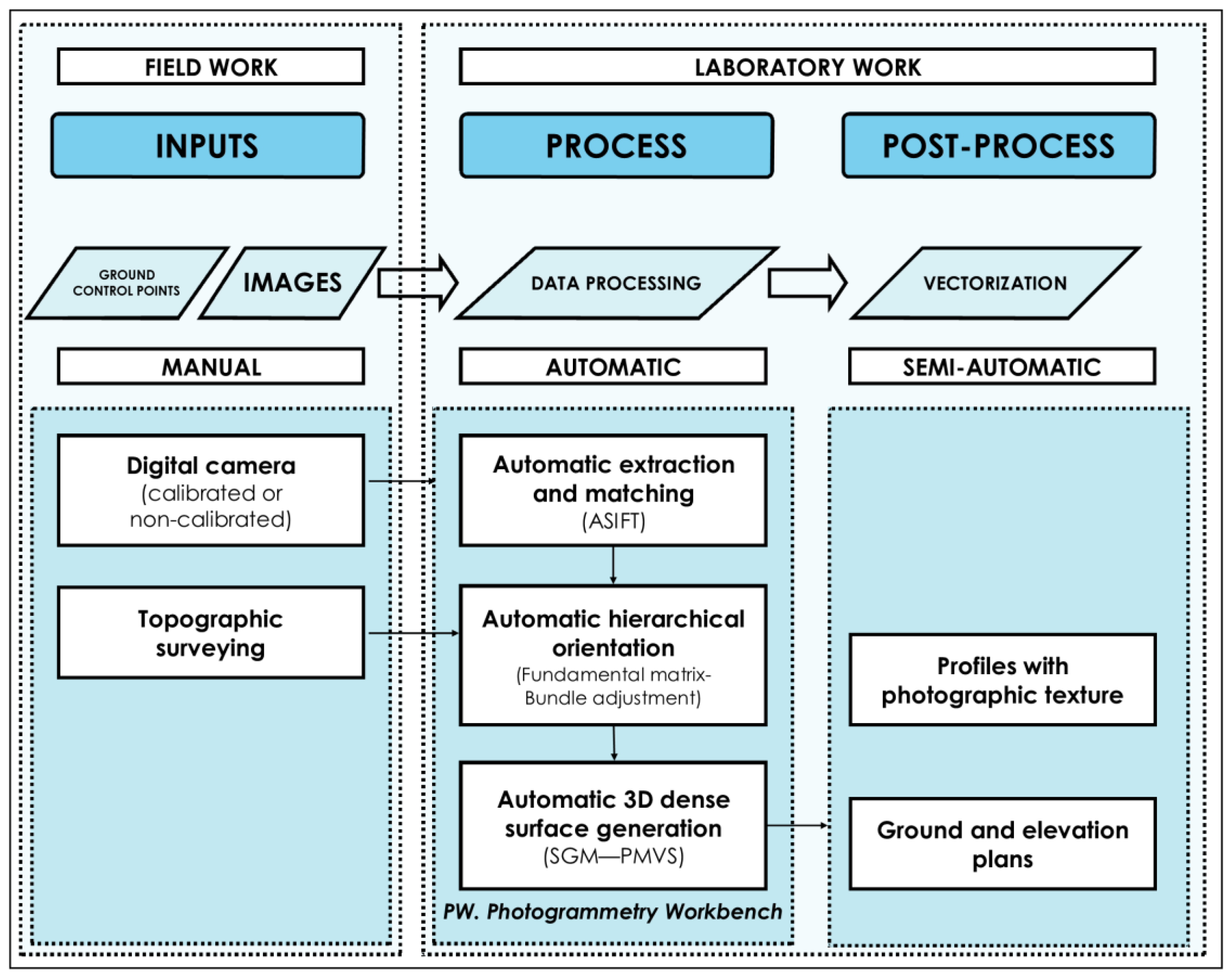
2. Methodology

From the capture of multiple images and after following a simple protocol, it is possible to obtain a non-manipulated 3D model, which allows the extraction of the relevant metric information of the building. However, one of the most critical steps in the process is the extraction and matching of the structural elements, lines and points, with high accuracy and reliability. These elements are the main support of the whole process, as they provide the necessary data to indirectly solve the spatial and angular position of the images (orientation), the camera self-calibration and the 3D reconstruction of the building. The following graphic (Figure 1) illustrates the steps taken in the 3D modeling from images.

2.1. Data Collection Protocol

The data collection in the form of images is the key to success, as it presents the input data of the process. The CIPA (Comite International de Photogrammetrie Architecturale) 3 × 3 Rules developed by [18] were designed to cope with image acquisition for the simple photogrammetric documentation of architecture. However, nowadays, the proliferation of digital cameras and the improvement of automatic algorithms have proven that these rules must be reformulated in terms of a higher number of images required. To this end, a specific image acquisition protocol has been designed for architectural modeling, which guarantees an easy and efficient data acquisition and ensures a dense surface reconstruction. Three different acquisition protocols are proposed in order to cope with as best as possible the size, morphology and external elements (i.e., occlusions, obstacles, etc.) of the buildings.

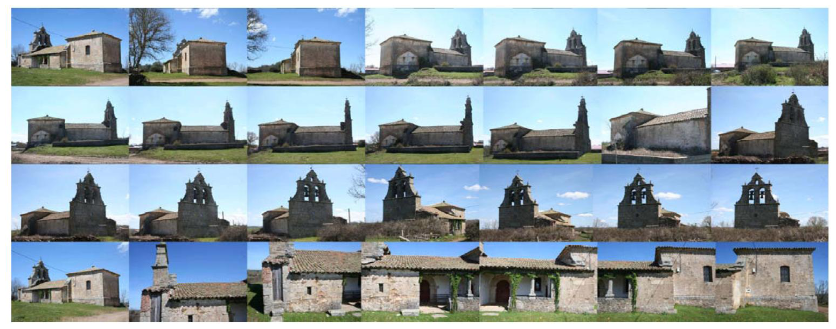
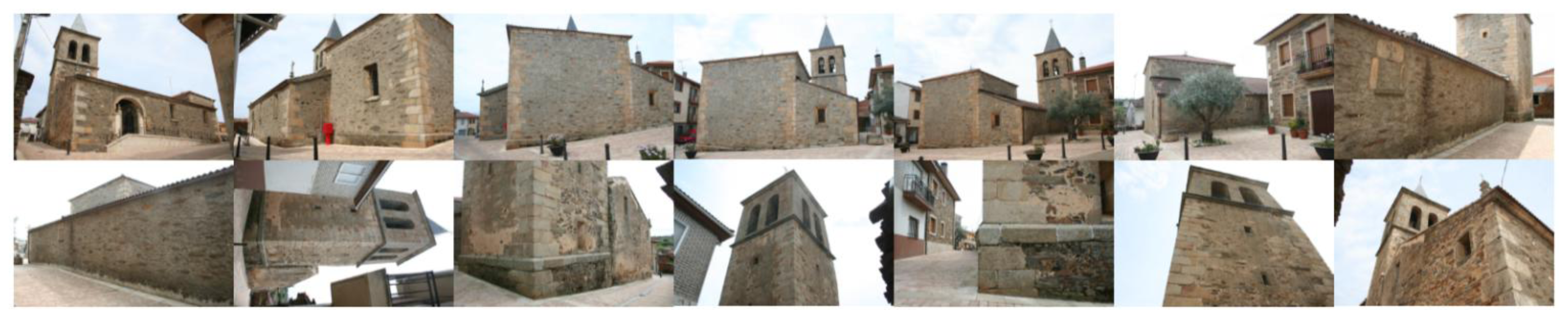
• Circular or “ring” network: used to obtain a 3D model of the whole building, which will then allow establishing the sections necessary to sketch the ground plan. The images axis must converge at the center of the object, and the minimum overlap between adjacent images must be about 80%. Moreover, the number of images in the corners should be higher, so that the user can “tie” the different façades of the object. The network of the shooting process should maintain an appropriate proportion between the base (distance between shots) and the distance to the object. As a general rule, in order to ensure image correspondence in the orientation process, the distance between two adjacent camera stations must be so that the camera axis forms an angle of intersection of approximately 15° with the object. The number of images necessary to obtain all of the measurements depends on the size, shape, morphology and location of the object (in relation to adjacent buildings) and the focal length (Figure 2, left).
• Planar or mosaic network: particularly recommended to document the façade of a building. It requires taking some frontal images of the façade, with an overlap higher than 80% between adjacent shots (Figure 2, center).
• Independent basic network: When documenting a small and accessible façade or any isolated architectonic element, the shooting network may consist of five images forming a cross with an overlap between adjacent shots higher than 90%. The main shot is a frontal image of the façade, which is then combined with four more images of the left, right, upper and lower part of the main shot, to conform a global, slight converging perspective (Figure 2, right).

Finally, in order to endow the object with metric properties, it is necessary to know the exact distance between two well-defined points in the image by measuring it with a tape measure or by incorporating some kind of surveying rod into the scene. That extra element must then appear in at least three images, so as to establish the scale of the model. Likewise, it should be highlighted the importance of choosing the output scale of the product, which will depend on the purpose and means of representation, as these determine the data capture [19]. Every scale entails a maximum accuracy, connected with the standard human eye acuity (0.2 mm).

Such accuracy matches the object pixel size or ground sample distance (GSD) through the following expression:

$$GSD=\frac{p·D}{f}$$

(1)

where D is the distance to the object, f the focal length and p the pixel size.

When using the digital camera, we only need to multiply the number of pixels along the height and width of the image by the GSD to get the object size covered by every frame. Besides, it is clear that the GSD, the pixel size and the focal length will determine the shooting distance to the object and the scale of the image.

In that way, depending on the maximum shooting distance, the size of the building and the minimum overlap between images, it will be possible to determine the number of images needed to fully document each face. However, in most cases, the maximum shooting distance is determined by the characteristics of the building location. Narrow streets, buildings, vehicles and vegetation near the object may block the way to getting the necessary distance to fit the whole building into the image. This means an increase in the number of images and sometimes in the maximum accuracy and, therefore, a larger scale in the final product, but it also means higher processing times and a higher probability of error.

2.2. Extraction and Matching of Features

The field of architectural documentation requires robust analysis for the extraction and correspondence of points of interest in the image, as the scale, perspective and lightning are variable. In the field of photogrammetry, the classic methods on correspondence between grey levels are ABM (area-based matching) [20] and LSM (least squares matching) [21]. However, for complex scenes, a more sophisticated and stable study is needed, which provides favorable and solid solutions to the geometric and radiometric variations. Such studies might be developed by applying algorithms, like SUSAN (smallest univalue segment assimilating nucleus) [22], SIFT (scale-invariant feature transform) [23], MSER (efficient maximally stable extremal region) [24] or SURF (Speeded Up Robust Features) [25]. Nevertheless, all of these new algorithms are not robust to the perspective variations of different images.

In this respect, a variation of the SIFT algorithm called ASIFT (affine scale-invariant transform) [26] has been added to the PW tool. The most remarkable improvement is the possibility of including two additional affinity parameters to control the perspective of the images, which correspond to the two perspective angles of the optical axis of the camera, ϖ (tilt) angle and ϕ (axis) angle (Equation (2)). The ASIFT algorithm will therefore allow working with images in perspective, which are frequent in these cases. The result is a descriptor, which stays the same regardless of the scale, rotation, movement and important deformations caused by the different perspectives of the images. The following expression accounts for the resulting descriptor:

$$A=\left[\begin{array}{cc}a& b\\ c& d\end{array}\right]=H_{\lambda }{R}_1(\kappa )T_1{R}_2(\varpi )=\lambda \left[\begin{array}{cc}\text{cos\hspace{0.17em}}\kappa & -\text{sin\hspace{0.17em}}\kappa \\ \text{sin\hspace{0.17em}}\kappa & \text{cos\hspace{0.17em}}\kappa \end{array}\right]·\left[\begin{array}{cc}t& 0\\ 0& 1\end{array}\right]·\left[\begin{array}{cc}\text{cos\hspace{0.17em}}\varpi & -\text{sin}\hspace{0.17em}\varpi \\ \text{sin}\hspace{0.17em}\varpi & \text{cos}\hspace{0.17em}\varpi \end{array}\right]$$

(2)

where A is the affine transformation with the scale λ, κ the rotation around the optical axis (swing) and the perspective parameters for the inclination of the optical axis of the camera: ϕ (tilt) = arccos (1/t), the angle between the optical axis and the normal to the image plane, and ϖ (axis), the azimuth angle between the optical axis and a fixed vertical plane.

The extraction of features is performed following the same SIFT workflow [27], but adding the two remarked perspective parameters (ϖ, ϕ), that is, the ASIFT descriptor incorporates a simulation of perspective caused by a variation of the camera optical axis direction. In particular, ASIFT proceeds by the following steps: (i) each image is converted by simulating all possible perspectives caused by the change of the camera’s optical axis orientation from a frontal position; (ii) these perspective rotations are performed from a finite and small number of tilt-ϕ and ϖ-axis angles; (iii) for each simulated image, the key points are extracted through gradient magnitude and orientation and based on histogram analysis for each pixel in a 4 × 4 neighborhood.

Finally, the matching process is carried out by the employment of the SIFT descriptors over the simulated images. These descriptors are matched firstly according to the Euclidean distance [23] and secondly filtered by the Moisan–Stival ORSA (optimized random sampling algorithm) [28]. This algorithm is a variant of RANSAC (Random Sample Consensus) [29] with an adaptive criterion to filter the mismatches by the employment of the epipolar geometry constraints.

2.3. Hierarchical Orientation of Images

After the extraction and matching of the aforementioned features, the orientation of the images is carried out by following a dual level that integrates computer vision with photogrammetry. The aim is to obtain an approximate orientation of the images within an arbitrary system of coordinates (computer vision), which may later be completely refined and improved for every image (photogrammetry).

First, it is necessary to carry out a relative orientation of the images through independent models by calculating the fundamental matrix using the Longuet–Higgins algorithm [30]. One of the main advantages of the fundamental matrix is that it is independent of the scene. Therefore, the matrix can be calculated from the point correspondence in the image and does not require knowing the internal parameters and initial approximations of the cameras. The fundamental matrix is defined by the following equation:

$${{\mathit{x}}^{\prime }}^{\text{T}}\mathbf{F}\mathit{x}=0$$

(3)

For each pair of matching points x_i ↔ x′_i (8 minimum), Equation (4) allows one to calculate the fundamental matrix. More specifically, by writing x = (x,y,1) and x′ = (x′,y′,1)^T, each matching point allows the creation of a linear equation,

$${\text{x}}^{\prime }{\text{xf}}_{11}+{\text{x}}^{\prime }{\text{yf}}_{12}+{\text{x}}^{\prime }{\text{f}}_{13}+{{\text{y}}^{\prime }\text{xf}}_{21}+{{\text{y}}^{\prime }\text{yf}}_{22}+{{\text{y}}^{\prime }\text{f}}_{23}+{\text{xf}}_{31}+{\text{yf}}_{32}+{\text{f}}_{33}=0$$

(4)

It should be noted that this procedure guarantees full automation in comparison with other photogrammetric approaches, where the user necessarily has to establish the initial approximations and also know the internal parameters of the camera. Horn [31] provides an algorithm to recover the baseline and relative orientation from the essential matrix, that is, assuming that an approximation for the geometric internal parameters of the camera (focal length and principal point) are available, i.e., the homogeneous 2D image coordinates are expressed as 3D photo vectors.

Second, once the relative angular and spatial position of the images is solved, we carry out a comprehensive bundle adjustment by means of an iterative and least-squares process based on the collinearity condition [5] and by adding the object coordinates to allow a full georeferencing of the images (Equation (5)). These object coordinates are incorporated into the orientation process thanks to the targets spread about the scene or by means of natural points, whose coordinates are measured by expeditious topographic survey (i.e., tape measure, manual measurement devices). In those cases when the internal calibration parameters (focal length, principal point and lens distortion) are unknown, this step enables us to add the calibration parameters of the camera to the equation as unknown quantities (self-calibration).

$$\begin{array}{l}(x-x_0)+\mathrm{\Delta }x=-f\frac{r_{11}(X-S_X)+r_{21}(Y-S_Y)+r_{31}(Z-S_Z)}{r_{13}(X-S_X)+r_{23}(Y-S_Y)+r_{33}(Z-S_Z)}\\ (y-y_0)+\mathrm{\Delta }y=-f\frac{r_{12}(X-S_X)+r_{22}(Y-S_Y)+r_{32}(Z-S_Z)}{r_{13}(X-S_X)+r_{23}(Y-S_Y)+r_{33}(Z-S_Z)}\end{array}$$

(5)

where x and y are the image coordinates; X, Y, Z are the object control points coordinates from the targets or natural points that allow the georeferencing of the scene; r_ij are the rotation matrix elements, which include the rotation of the camera; S_X, S_Y, S_Z are the object coordinates of the points of view of the camera; f is the principal distance; x₀, y₀ the principal point coordinates of the image; and ΔX, ΔY the translations due to the radial and tangential distortion of the lens according to Equation (6).

$$\begin{array}{l}\mathrm{\Delta }x=-x_p-\frac{x^{\prime }}{f}\mathrm{\Delta }f+x^{\prime }\left(r^2{k}_1+r^4{k}_2+r^6{k}_3\right)+\left(2{x^{\prime }}^2+r^2\right)p_1+2p_2{x}^{\prime }{y}^{\prime }+b_1{x}^{\prime }+b_2{y}^{\prime }\\ \mathrm{\Delta }y=-y_p-\frac{y^{\prime }}{f}\mathrm{\Delta }f+y^{\prime }\left(r^2{k}_1+r^4{k}_2+r^6{k}_3\right)+2p_1{x}^{\prime }{y}^{\prime }\left(2{y^{\prime }}^2+r^2\right)p_2\end{array}$$

(6)

This is the Fraser model [32], which takes into account additional parameters compared to the Gaussian distortion model [33]: besides the principal distance (f) and principal point coordinates (x_p, y_p), the radial distortion (k₁, k₂, k₃) and tangential distortion (p₁, p₂) parameters are included. Furthermore it considers terms for affinity (b₁) and non-orthogonality (b₂).

Two important considerations must be taken into account: (a) the bundle adjustment can be carried out with or without the knowledge of the camera’s parameters. In the first case, the interior and the lens distortion parameters are entered by their known value. In the second case, they must be considered as unknown (self-calibration) and solved with the whole set of unknowns; (b) this is the moment in which an absolute datum can be defined. This can be done by means of the object coordinates of ground control points measured with any topographic method or even by means of geometric constraints that define the 7 parameters of the coordinate frame.

2.4. Dense Model Generation

On the basis of the robust orientation of the image, a dense matching process has been developed. Depending on the geometry of the shooting configuration, the process will use either an SGM or a PMVS strategy by means of the projectivity Equation (7) [12]. This allows generating a dense model capable of determining the exact 3D coordinate of the object for each pixel.

$$x_k=C\left(D\left(R_i\left(X_k-S_i\right)\right)\right)$$

(7)

where X is the object point, x the corresponding point in the image, R the camera rotation matrix, S the center of projection of the camera, C the internal calibration function and D the lens distortion function; and the k and i subscripts refer to the point and the image, respectively.

The SGM process consists of minimizing an energy function (8) along the 8 basic directions of a pixel (every 45°). This function consists of a cost function, M (pixel matching cost), which accounts for the degree of similarity of the pixels between two images, x and x′, and the inclusion of two restrictions, P₁ and P₂, which account for potential gross errors in the SGM process. In addition, a further restriction based on the epipolar geometry of photogrammetry [34] has been added to the SGM process. This restriction allows limiting the search space for each pixel, so that the high computational cost of generating a dense model from multiple images is reduced, thus achieving better processing times.

$$E(D)=\sum _x\left(M(x,D_x)+\sum _{x^{\prime }\in N_x}{P}_{1}T\left(\left|D_x-D_{x^{\prime }}\right|=1\right)+\sum _{x^{\prime }\in N_x}{P}_{2}T\left(\left|D_x-D_{x^{\prime }}\right|>1\right)\right)$$

(8)

where E(D) represents the energy function to be minimized on the basis of disparity (parallax) between matching features; function C (pixel matching cost) evaluates the degree of similarity between pixel p and its correspondent q by means of its disparity or parallax D_p; the terms P₁ and P₂ represent two restrictions, which avoid potential gross errors in the dense matching process caused by disparities in one or more pixels.

On the other hand, the PMVS method allows obtaining a dense model through a hierarchical and sequential process, which includes matching, expansion and filtering. In the matching phase, the points of interest and corners are extracted by applying the Harris [35] and the difference-of-Gaussian (DoG) operators. Later, a multiple image matching process is carried out on the basis of the previous extraction and the normalized cross-correction (NCC) operator [36]. After the initial matching, expansion and filtering functions are applied, which allow extending the initial matching to the nearest pixels, as well as detecting and deleting erroneous matches by applying visibility restrictions.

3. Results and Discussion

3.1. Context

The area of study is the region of Aliste (Zamora), with a total of 33 towns grouped into six municipalities. The region of Aliste is located to the west of the province of Zamora (Spain), bounded on the north by the mountain range of “La Culebra”, and adjacent to the regions of Sanabria and La Carballeda. It is bordered to the east by the regions of “Tierras de Tábara” and “Tierras de Alba”, and to the south by the region of Sayago. The west is adjacent to the Portuguese border, in the area known as “la raya” (“The line”). Such a location highlights the outlying position, both geographic and socioeconomically, which has marked the region throughout time. This area has been chosen due to its geographical location, near the Portuguese border and the region of Sanabria, of which there are previous similar studies. Therefore, it is possible to undertake comparative studies of the different typologies of religious buildings. A total of 32 parish churches and five chapels have been analyzed (

Table 1. Towns under analysis.

Municipality	Town	Municipality	Town	Municipality	Town
ALCAÑICES	Alcañices	FONFRIA	Fonfría	RABANO	Rábano de Aliste
	Alcorcillo		Arcillera		San Mamed
	Santa Ana		Bermillo de Alba		Sejas de Aliste
	Vivinera		Brandilanes		Tola
FIGUERUELA	Figueruela de Arriba		Castro de Alcañices	TRABAZOS	Trabazos
	Figueruela de Abajo		Ceadea		Latedo
	Gallegos del Campo		Fornillos		Nuez de Aliste
	Moldones		Moveros		San Martín del Pedroso
	Riomanzanas		Salto de Castro		Villarino tras la Sierra
	Villarino de Manzanas	VINAS	Viñas de Aliste
	Flechas		Ribas
			San Blas
			Vega de Nuez

).

Due to its location, the region of Aliste has always been a border area between different people and cultures. The presence of Arabs in the area led to the depopulation of the Douro Valley, although the subsequent Christian advance in the ninth century brought the population back. The emergence of new monasteries inhabited by monks from the south of the Peninsula, who came to occupy the conquered territories, was of central importance. That is how a series of monasteries arose, which gave new value to fields that had not been farmed or were abandoned. In the same way, the individuals, nobles and priests carried out a rural repopulation through the establishment of churches that fostered rural development, thus promoting the creation of parish churches. Parish churches were not only a religious center for the population, but also the center of administrative, social, economic and cultural activities of the community.

The towns in Aliste were part of the Diocese of Braga until 1297, when the Treaty of Alcañices transferred them to the Kingdom of León, thus creating the border with Portugal. The Templar Knights settled in Aliste during the expansion of religious orders all over the Iberian Peninsula, which began in the 13th century. In the 14th century, Aliste joined the Diocese of Santiago, after being part of the Diocese of Astorga. Finally, in the 19th century, it joined the Diocese of Zamora.

3.2. Fieldwork

The method chosen to carry out the fieldwork is supposed to allow the documentation of a great amount of buildings in a relatively short period of time (at least five churches per day). Moreover, the cost is minimum (only a digital camera and a metric tape is necessary), and one person is enough for the dataset acquisition.

The aim is to generate the necessary graphic documentation to carry out a typological study of the religious buildings of the border municipalities in the region of Aliste (Zamora). The results are presented in the form of ground plans and profiles with photographic texture and axonometric view. The output scale is 1/200, as such documentation may be included in what several authors refer to as the “preliminary level of documentation” [37,38], this being the minimum scale recommended. The scale demands a minimum accuracy of 40 mm.

The photos were taken with a reflex camera, Canon EOS 350D, set to the lowest ISO and with an aperture in the range from f/4 to f/5. Moreover, the focal length, 18 mm, was fixed throughout the shooting process. According to Equation (1), a 1/200 scale allows a maximum distance to the object of 112.5 m, which means a footprint of 138 × 92 m in every shot. Therefore, the shooting distance is lower than the maximum recommended, thus guaranteeing a higher accuracy than the minimum required for the 1/200 scale. However, the major problem was the width of the streets that surrounded the churches, as they define the maximum distance allowed to take the photos, as well as the part of the scene that can fit into every image and, therefore, the minimum number of images needed.

The circular or “ring” shot strategy was used for documenting the building, trying to maintain a constant distance to the building. The images’ network around the building is designed to keep an appropriate proportion between the distance to the object and the distance between images, which is around 0.26 (Figure 3). This factor is the result of calculating the tangent of the 15° angle of intersection with the object, referred to in Subsection 2.1. This factor is important for the generation of dense models, since it guarantees small baselines between cameras and, thus, a fully documented point cloud.

Every church had external conditioning factors (e.g., narrow perimeter streets, fences, private properties, etc.), which made it impossible to fit the whole object into the image, at least for one of the façades. In such cases, a planar or mosaic shot of the area was performed, making sure that the images had an overlap rate of at least 80%. We made sure of having convergent (oblique) images to “tie” the circular shots and the mosaic shots in order to obtain a precise orientation.

According to Figure 3, the best scenario was the church in Ceadea. The fact that the church is isolated from the urban area, small and low, made it possible to take the photos at a sufficient distance to close the ring with just 28 shots, which includes the roofs of the building. The mosaic network was used only for the south façade, as the minimum distance was five meters (the six last images in Figure 4). The other churches were part of the urban area and were adjacent to other buildings, which made it impossible to fit the whole image in one single shot, thus forcing us to take more photos with an overlap rate of 80%. On the other side, the worst scenario was the church in Trabazos, which is one of the biggest churches in our study. It has a high belfry tower and three façades facing narrow streets three to four meters wide, which forced us to take 177 photos in order to close the shooting ring around the building. We had to use the mosaic network technique for every façade, except for the eastern one, which faces a big square (Figure 4).

Finally, the distance between two points in the images were measured so as to establish the metric requirements of the 3D model, which was later created in the laboratory. Simple methods (tape measure, manual measurement devices) were used to measure the distance between two distant points for each of the building faces. However, this step may be skipped by incorporating some kind of stake, whose size must be known and which must appear in at least three images to allow the establishing of the scale of the model.

3.3. Laboratory Work

We used PW for the laboratory work, which allows us to generate the 3D models that determine the outside geometry of the church and, therefore, the scaled 3D models and the resulting photo-realistic profiles. The interior of the churches has not been modeled through a rigorous photogrammetric procedure. Instead, the most important features (e.g., wall thickness and internal distances) were measured with tape measure in order to complete the ground plans of every church.

Following the aforementioned workflow (Figure 1), the automatic orientation of the images was undertaken, which resulted in a scattered point cloud (Figure 5, left). Then, the erroneous points were deleted for a better outcome. Afterwards, a dense point cloud was automatically generated (Figure 5, right).

In order to generate the dense point cloud of the church in Ceadea, 28 images were used, while in the case of Trabazos, 121 images were used (those more perpendicular to the faces to be modeled). Due to the different geometric characteristics and the external conditions in both buildings, the roofs of the church in Ceadea were modeled, thanks to the shooting distance. However, the modeling of the church in Trabazos was not possible, because of the adjacent buildings and the height of the church. On the contrary, and due to the proximity to the faces, the point density is higher in the model of Trabazos, and therefore, the level of detail is higher than that of the church in Ceadea.

After removing noise from the images, the point cloud was divided into sections in order to outline the ground plan and export it to a CAD program, so as to draw the geometry. Moreover, we obtained the orthogonal profiles of the façades and then processed them with a CAD program to get the final product (Figure 6).

The main technical data obtained in the processing phase are recorded in

Table 2. Main technical data obtained from the processing of the ten case studies. GSD, ground sample distance.

	Fornillos	Vivinera	Rabano	Tola	Trabazos	Sejas	Santa Ana	Ribas	Ceadea	S. Martin Pedroso
FIELDWORK
Measurements (m)	25 × 16 × 20	18 × 16 × 12	21 × 13 × 12	22 × 16 × 14	27 × 16 × 23	32 × 17 × 22	20 × 15 × 10	23 × 16 × 11	19 × 10 × 11	22 × 15 × 13
No. of images	86	72	127	152	177	78	38	91	28	79
Distance max/min (m)	22.40/10.30	16.20/4.50	30.80/3.50	25.30/2.90	25.30/2.60	16.50/2.80	15.10/4.50	19.30/9.70	30.15/5.20	31.10/5.70
Fieldwork (minutes)	45	40	50	60	70	45	35	40	30	45
LABORATORY WORK
Tie points	227,666	252,895	407,975	651,467	429,726	353,976	188,221	249,567	82,149	224,492
No. of 3D points	22,319,921	20,913,054	39,624,832	53,447,764	44,416,441	25,141,761	11,138,274	17,894,546	4,854,354	17,302,829
GSD (m)	0.008	0.007	0.006	0.006	0.006	0.006	0.006	0.008	0.007	0.008
RMSE (m/pix)	0.0022/0.28	0.0014/0.26	0.0018/0.31	0.0037/0.33	0.0011/0.18	0.0017/0.28	0.0015/0.26	0.0023/0.30	0.0015/0.22	0.0022/0.29
Laboratory work (hours)	14	10	15	15	17	16	7	12	6	12

.

The number of images for each model reflects the size of the building and the characteristics of its surroundings. The time spent on fieldwork is determined by the number of images and the use of a tripod depending on the lightning conditions. The time spent on laboratory work can be divided into two phases. The first phase consists of masking the images by hand, whereas the image orientation and the generation of the dense point cloud are completed automatically. The time spent on these processes is directly related to the number of images. The second phase consists of removing noise from the model, generating the orthophotos and outlining the plans. In this case, the amount of time depends on the size of the church.

Once the graphic data of every church is collected, a typological study of the buildings, together with its classification in families, types and variants, is carried out.

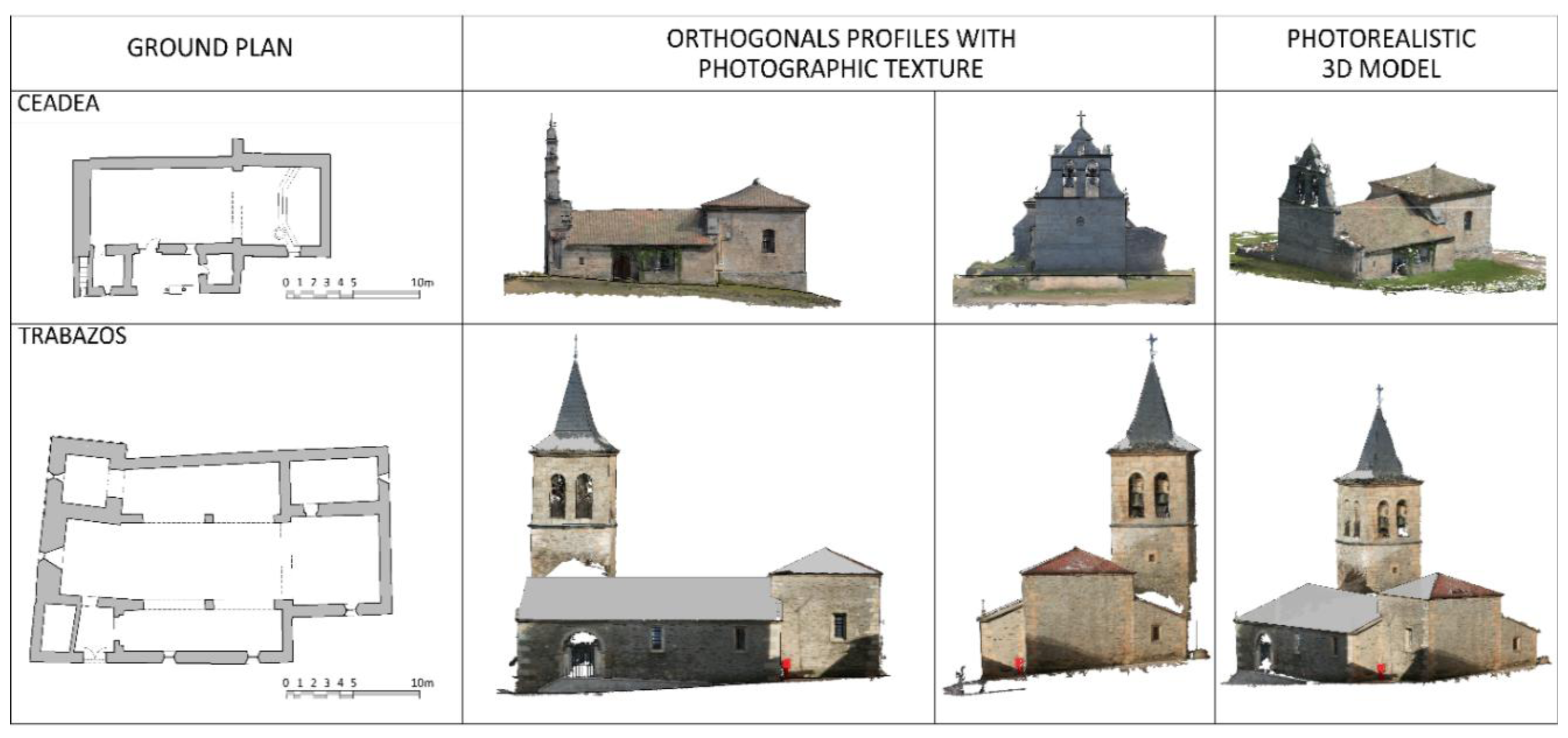
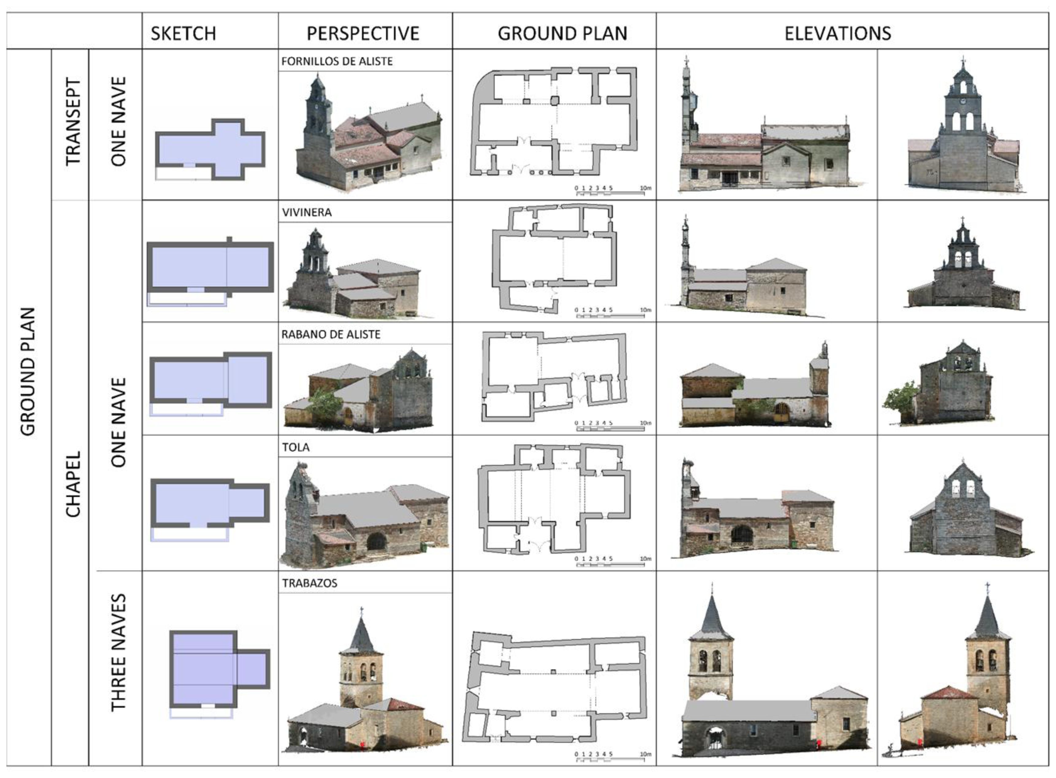
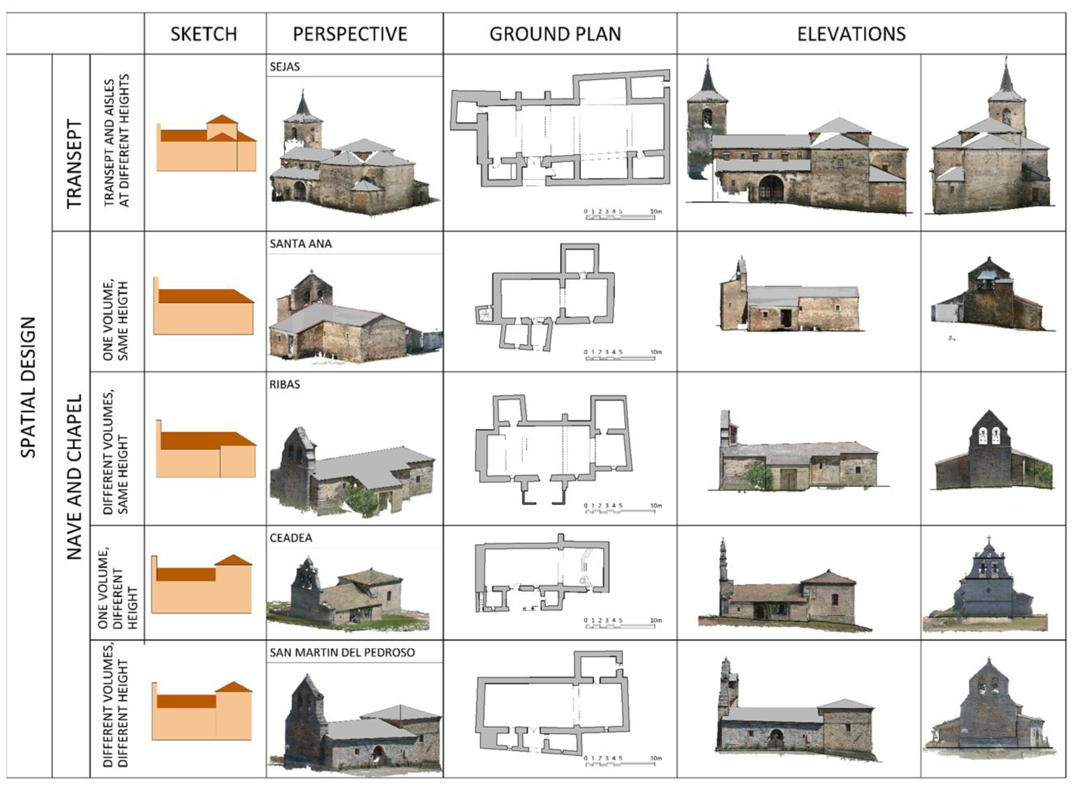
3.4. Typological Analysis

The working line followed by San José (1994) [39] has been a point of reference for the typological analysis. A similar study for the religious buildings of the border towns in the area of Aliste has been developed, though in this case, the last generation of low-cost photogrammetric and computer vision methods both in the shooting process and the generation of 3D models have been used. In order to classify the churches, the starting point were the families, which are made up of the different building systems, and these, in turn, divided into subsystems and variants. The study was limited to the classification of the parish churches in the rural areas of Aliste, as they are the most numerous and representative group.

The parish churches have been classified according to the study of their ground plans, by means of analyzing the layout of the essential architectural elements: nave, chapel and transept. As a result, two groups or families have been established: churches with transept and churches with chapel. From these two groups, the different types of churches in the area were classified according to the number of naves, which resulted in new subtypes. The variants were established according to the size of the essential structures, the layout of the belfry and the complementary architectural elements attached to the main structure (e.g., chapels, sacristy, arcade, etc.).

The methodology adopted for the typological analysis of the churches consisted of visiting and studying each temple to establish by means of comparison the different types. For this, the study is based on the structures that make up the temples and the way in which they are linked together. Thus, the first classification is attained: temples with transept and temples with chapel. On this basis, the number of naves determines the variants or subtypes.

With regard to the classification, the differences previously established on the basis of shape, number and arrangement, linked together to shape the temple, are essential for gathering the studied buildings into groups with similar characteristics. This results in the final classification of the different types and its classification into typologies and variants. Thirty two parish churches and five chapels have been analyzed, and the typological classification of the churches has been outlined in accordance to the layout of the nave and either the chapel or transepts, as well as its size. We have chosen one church from each group to be included in the results (Figures 7 and 8). The parish churches consisting of one single nave and a chapel are by far the most numerous group of religious architecture in the area. The structure includes the rectangular ground plan of the nave and the square ground plan of the main chapel, which, according to Christian tradition, is oriented east-west. The final structure results from attaching the supplementary architectural elements, such as entrance arches, sacristy, belfry, etc., to the main structure. The belfry is especially relevant in the volumetric configuration of the temples. In this study, every church is crowned by a bell gable, though there are different types.

With regard to the building system, these churches are simple constructions consisting of perimeter load-bearing walls and semicircular arches in the junction between the nave and the chapel. The roof consists of a wood couple roof (a gabled roof in the nave and a hipped roof in the chapel) in those cases where the chapel is higher than the nave.

The variants of this type of buildings are determined by the volumetric ratio between the nave and the chapel (Figure 8). Therefore, there are some churches in which the nave and chapel are the same size and height, others where the nave and the chapel have the same width, but the chapel is higher than the nave and, finally, those where the nave and the chapel have different sizes and heights. The most numerous group within the churches in this study belong to the latter group, thus being the prevailing typology of religious architecture in the area. The last variation would be a church where the chapel and the nave have a different width and height, thus creating two well-differentiated parts within the essential spaces of the temple.

The group made up of churches with three naves and one chapel is the less numerous one. The structure consists of two side naves attached to the main nave and chapel, which are accessed from the central nave through semicircular arches on columns.

The parish churches of one nave and crossing are the biggest ones and are normally located in the most populated towns.

4. Conclusions

The study shows the capacity of photogrammetric programs, which are aimed towards the full automation of the cartographic modeling process, for the architectural interpretation of religious buildings. By means of a relatively simple working methodology, used both in the shooting and processing phase, accurate and high graphic quality results can be obtained. Thanks to photogrammetric tools, the aim of creating a typological classification of the parish churches in the region of Aliste has been made easier and is based on technical data.

The following conclusions from the present study can be drawn:

(a)

The graphic quality of the models is supported basically by the point quantity, between 20 and 50 million points, which usually equals or surpasses the resolution provided by terrestrial laser systems (TLS).

(b)

Even though the data volume may seem high, the working times must be taken into account: between 30 and 60 min of fieldwork and from 6 to 16 h of laboratory work, which, once again, can be compared with laser scanner performance. The image capture times are lower than those of a laser scanner (between 1/2 and 1/3 depending on the TLS performance), whereas the laboratory work times are similar. Therefore, compared to laser scanner technology in terms of devices availability and the difficulty of processes, photogrammetry stands out as a more advantageous solution.

(c)

The high degree of accuracy (root mean square deviation of block adjustment; the results range from 1/4 to 1/3 of a pixel) is mainly due to the high level of redundancies (high number of tie points), which allows the user to adjust the images accurately

(d)

The high level of redundancies (tie points), between 80,000 and 650,000 with an average of about 300,000, is due to the high number of images, between 28 and 177 with an average of about 90. Although the number of images may seem excessive, this issue must be contrasted to the time spent in the process.

(e)

The results are highly consistent with each other: RMS are always between 0.18 and 0.33 pixels or between 0.0011 and 0.0037 mm, which guarantee the quality and reliability of the methodology chosen for the study.

(f)

The different number of images needed for each church, which ranges from 28 to 177, as stated before, depends on the surroundings of the religious building, as well as on the possibility of fitting the whole object into the image. The size of the building is also important, although all the different aspects do not result in relevant differences, either in time or accuracy.

(g)

With regard to the typological analysis, the approach developed improves the current techniques for the recording of architectural cultural heritage. Moreover, the method is suitable to carry out a typological classification study, where the reduction of image capture times (between 1/2 and 1/3, as stated above) allows the researcher to document a great number of buildings/architectural heritage in little time and by non-specialist staff, due to the simplicity of the process. Besides, the high resolution of the models, with GSDs between 0.006 and 0.008 mm, indicates that the method could be used for projects that require larger scales.

(h)

These methods are appealing to architects due to their simplicity and speed. Better quality and more robust surveys are obtained, as not only the shape of the building was accessed, but also the information about its color and texture. The fieldwork hours are reduced with no negative effect on accuracy, and it is easier to systematize the process, by following the protocol set out in the present study.

With regard to future action lines, it is worth mentioning:

The aim would be to apply the methodology to other contexts and architectural typologies, in order to compare the scope and validity of the method. This could lead to the creation of a good practices guide to help the inexperienced user choose a line of action that optimizes the relation between accuracy and working time.

It will be important to look at further ways of adding any type of metric constraint to the methodology, so as to avoid manual measuring between several points of the object, thus reducing the working times and, more importantly, reducing the potential sources of error.

Finally, the implementation of processing strategies that enable progress on the automation of point clouds should also be undertaken, in order to facilitate the process of turning point clouds into vector models.

References

- Haala, N.; Peter, M.; Kremer, J.; Hunter, G. Mobile lidar mapping for 3D point cloud collection in urban areas—A performance test. Int. Arch. Photogramm. Remote Sens. Spat. Inf. Sci 2008, 37, 1119–1127. [Google Scholar]
- Schindler, K. An overview and comparison of smooth labeling methods for land-cover classification. IEEE Trans. Geosci. Remote Sensi 2012, 50, 4534–4545. [Google Scholar]
- Liu, G.-H.; Liu, X.-Y.; Feng, Q.-Y. High-accuracy three-dimensional shape acquisition of a large-scale object from multiple uncalibrated camera views. Appl. Opt 2011, 50, 3691–3702. [Google Scholar]
- Gruen, A.; Akca, D. Mobile Photogrammetry. In Dreiländertagung SGPBF, DGPF und OVG, Proceedings of 2007 Wissenschaftlich-Technische Jahrestagung der DGPF, Muttenz, Basel, 19–21 June 2007; 16, pp. 441–451.
- Kraus, K. Photogrammetry. Fundamentals and Standard Processes; Dummlers Verlag: Bonn, Germany, 1993; Volume 1. [Google Scholar]
- Arias, P.; Caamano, J.C.; Lorenzo, H.; Armesto, J. 3D modeling and section properties of ancient irregular timber structures by means of digital photogrammetry. MICE Comput.-Aided Civ. Infrastruct. Eng 2007, 22, 597–611. [Google Scholar]
- Lorenzo, H.; Arias, P. A methodology for rapid archaeological site documentation using ground-penetrating radar and terrestrial photogrammetry. Geoarchaeology 2005, 20, 521–535. [Google Scholar]
- Arias, P.; Armesto, J.; Vallejo, J.; Lorenzo, H. Close range digital photogrammetry and software application development for planar patterns computation. Dyna 2009, 76, 7–15. [Google Scholar]
- Robertson, D.P.; Cipolla, R. Structure from Motion. In Practical Image Processing and Computer Vision; John Wiley: Hoboken, NJ, USA, 2009; p. 49. [Google Scholar]
- Quan, L. Image-Based Modeling; Springer: New York, NY, USA, 2010. [Google Scholar]
- Szeliski, R. Computer Vision: Algorithms and Applications; Springer: New York, NY, USA, 2011; p. 824. [Google Scholar]
- Hartley, R.; Zisserman, A. Multiple View Geometry in Computer Vision; Cambridge University Press: Cambridge, UK, 2000. [Google Scholar]
- Hirschmüller, H. Accurate and Efficient Stereo Processing by Semi-Global Matching and Mutual Information. Proceedings of the 2005 IEEE Computer Society Conference on Computer Vision and Pattern Recognition, San Diego, CA, USA, 20–25 June 2005.
- Deseilligny, M.P.; Clery, I. Apero, an Open Source Bundle Adjusment Software for Automatic Calibration and Orientation of Set of Images. Proceedings of the 2011 ISPRS Commission V Symposium, Image Engineering and Vision Metrology, Trento, Italy, 2–4 March 2011; XXXVIII-5/W16, pp. 269–276.
- Habbecke, M.; Kobbelt, L. Iterative Multi-View Plane Fitting. Proceedings of the 2006 International Fall Work-Shop Vision, Modeling, and Visualization, Aachen, Germany, 22–24 November 2006; pp. 73–80.
- Seitz, S.M.; Curless, B.; Diebel, J.; Scharstein, D.; Szeliski, R. A Comparison and Evaluation of Multi-View Stereo Reconstruction Algorithms. Proceedings of the 2006 IEEE Computer Society Conference on Computer Vision and Pattern Recognition, Washington, DC, USA, 17–22 June 2006; 1, pp. 519–528.
- Furukawa, Y.; Ponce, J. Accurate, dense, and robust multiview stereopsis. IEEE Trans. Pattern Anal. Mach. Intell 2010, 32, 1362–1376. [Google Scholar]
- Waldhäusl, P.; Ogleby, C. 3 × 3 rules for simple photogrammetric documentation of architecture. Int. Arch. Photogramm. Remote Sens 1994, 30, 426–429. [Google Scholar]
- Patias, P.; Santana Quintero, M. Introduction to Heritage Documentation. In CIPA Heritage Documentation Best Practices and Applications; Stylianidis, E., Patias, P., Santana Quintero, M., Eds.; The ICOMOS & ISPRS Committee for Documentation of Cultural Heritage: Athens, Greece, 2011; Volume XXXVIII-5/C19, pp. 9–13. [Google Scholar]
- Joglekar, J.; Gedam, S.S. Area based image matching methods—A survey. Int. J. Emerg. Technol. Adv. Eng 2012, 2, 130–136. [Google Scholar]
- Gruen, A. Adaptive least squares correlation: A powerful image matching technique. S. Afr. J. Photogramm. Remote Sens. Cartogr 1985, 14, 175–187. [Google Scholar]
- Smith, S.M.; Brady, J.M. Susan—A new approach to low level image processing. Int. J. Comput. Vis 1997, 23, 45–78. [Google Scholar]
- Lowe, D.G. Object Recognition from Local Scale-Invariant Features. Proceedings of the 1999 IEEE International Conference on Computer Vision, Kerkyra, Greece, 20–27 September 1999; 2, pp. 1150–1157.
- Matas, J.; Chum, O.; Urban, M.; Pajdla, T. Robust Wide Baseline Stereo from Maximally Stable Extremal Regions. Procceding of the 2002 British Machine Vision Conference, Citeseer, Cardiff, UK, 2–5 September 2002; pp. 384–393.
- Bay, H.; Ess, A.; Tuytelaars, T.; van Gool, L. Speeded-up robust features (surf). Comput. Vis. Image Underst 2008, 110, 346–359. [Google Scholar]
- Morel, J.-M.; Yu, G. Asift: A new framework for fully affine invariant image comparison. SIAM J. Imaging Sci 2009, 2, 438–469. [Google Scholar]
- Lowe, D.G. Distinctive image features from scale-invariant keypoints. Int. J. Comput. Vis 2004, 60, 91–110. [Google Scholar]
- Moisan, L.; Stival, B. A probabilistic criterion to detect rigid point matches between two images and estimate the fundamental matrix. Int. J. Comput. Vis 2004, 57, 201–218. [Google Scholar]
- Fischler, M.A.; Bolles, R.C. Random sample consensus: A paradigm for model fitting with applications to image analysis and automated cartography. Commun. ACM 1981, 24, 381–395. [Google Scholar]
- Longuet-Higgins, H.C. A computer algorithm for reconstructing a scene from two projections. Nature 1981, 293, 133–135. [Google Scholar]
- Horn, B.K.P. Recovering baseline and orientation from essential matrix. J. Opt. Soc. Am 1990, 1–10. [Google Scholar]
- Fraser, C.S.; Shortis, M.R.; Ganci, G. Sensor and System Calibration. In Multisensor System Self-Calibration; Society of Photo-Optical Instrumentation Engineers (SPIE): Philadelphia, PA, USA, 1995; pp. 2–18. [Google Scholar]
- Brown, D. Close-range camera calibration. Photogramm. Eng 1971, 37, 855–866. [Google Scholar]
- Luhmann, T.; Robson, S.; Kyle, S.; Harley, I. Close Range Photogrammetry: Principles, Methods and Applications; Whittles: Dunbeath, UK, 2007; p. 528. [Google Scholar]
- Harris, C.; Stephens, M. A Combined Corner and Edge Detector. In The Fourth Alvey Vision Conference; University of Sheffield Printing Office: Manchester, UK, 1988; pp. 147–151. [Google Scholar]
- González, R.C.; Woods, R.E. Digital Image Processing, 3rd ed; Addison-Wesley: Massachusetts, MA, USA, 1992. [Google Scholar]
- Almagro Gorbea, A. Levantamiento Arquitectónico; Universidad de Granada: Granada, Spain, 2004. [Google Scholar]
- Letellier, R.; Schmid, W.; LeBlanc, F.; Eppich, R.; Chabbi, A. Recording, Documentation, and Information Management for the Conservation of Heritage Places: Guiding Principles; Getty Conservation Institute: Los Angeles, CA, USA, 2007. [Google Scholar]
- San José Alonso, J.I. Arquitectura Religiosa en Sanabria: Sus Espacios, Organizaciones y Tipologías; Instituto de Estudios Zamoranos Florián de Ocampo: Zamora, Spain, 1994. [Google Scholar]