3D Ground Penetrating Radar to Detect Tree Roots and Estimate Root Biomass in the Field

Abstract

The objectives of this study were to detect coarse tree root and to estimate root biomass in the field by using an advanced 3D Ground Penetrating Radar (3D GPR) system. This study obtained full-resolution 3D imaging results of tree root system using 500 MHz and 800 MHz bow-tie antennas, respectively. The measurement site included two larch trees, and one of them was excavated after GPR measurements. In this paper, a searching algorithm, based on the continuity of pixel intensity along the root in 3D space, is proposed, and two coarse roots whose diameters are more than 5 cm were detected and delineated correctly. Based on the detection results and the measured root biomass, a linear regression model is proposed to estimate the total root biomass in different depth ranges, and the total error was less than 10%. Additionally, based on the detected root samples, a new index named “magnitude width” is proposed to estimate the root diameter that has good correlation with root diameter compared with other common GPR indexes. This index also provides direct measurement of the root diameter with 13%–16% error, providing reasonable and practical root diameter estimation especially in the field.

1. Introduction

Ground Penetrating Radar (GPR), as a convenient, nondestructive technique to acquire subsurface information, has been successfully used in many engineering applications in detection and localization of subsurface targets (e.g., landmine, pipelines, and cables) [1–4]. Although there are various novel methods used to study root system of vegetation [5–9], GPR has become a popular and common tool to detect coarse root and estimate root biomass in the last decade. Especially, Guo et al. reviewed these applications of GPR for coarse root detection and root biomass estimation in detail, and summarized various methods and experiences for detecting and quantifying roots from the acquired GPR data, mostly in controlled conditions [10]. The main purpose of root detection, using GPR is, to extract roots from GPR profiles and reconstruct the architecture of root systems. Hruska et al. firstly mapped tree root systems using a GPR system with a central frequency of 450 MHz [5]. Although the three-dimensional (3D) views were delineated manually based on the different GPR profiles after signal processing, it still verified the feasibility of the GPR technique for root detection. Subsequently, many studies on 3D reconstruction of root systems by GPR were carried out [11–13]. However, the scanning grids usually were too sparse in the measurements to satisfy the Nyquist spatial sampling criterion, which would result in spatial aliasing of the 3D migrated results. Actually, these above-mentioned studies also demonstrated that only coarse roots could be detected and the clustering of fine roots was not detectable individually in the field. Furthermore, Hirano et al. analyzed these important factors, in the coarse root detection, using GPR quantitatively, including root diameter, root water content, and intervals between roots [14]. In addition to the architecture reconstruction of root system using GPR, root biomass estimation is also very important for understanding carbon storage in terrestrial ecosystems. Commonly, root biomass estimation using GPR can be classified as two kinds of approaches [10]: one is to estimate the coarse root biomass from the GPR reflection intensity indexes directly; the other is to estimate the diameter of the coarse root first, and then combine prior information of root density to calculate the root biomass indirectly. For the first kind of approach, some indexes usually calculated from the GPR profiles after migration and Hilbert transform were validated to correlate with the root biomass, which include areas within threshold range, pixels within threshold range, mean pixel intensity, high amplitude area, and so on [15–17]. The second kind of approach is mainly based on an assumption that the shape of root is cylindrical. Cui et al. reported the strong positive correlation between root biomass and root diameter, and verified that root biomass estimation is equivalent to root diameter estimation [18]. Some similar indexes, such as high amplitude area, time intervals between zeros-crossings of waveform, and pixels within the threshold range were also verified to correlate with root diameter well [14,15,19]. Hence, some linear or multiple regression models were built for estimating the root diameter by these extracted indexes [18,20]. In recent years, the GPR technique becomes more and more popular, and widely-used in the study of tree root systems, which has been an important application of GPR [21–26].

Soil in the field is typically a heterogeneous and lossy complex media, and its dielectric properties vary greatly and change with different water content. A tree root is one of quasi-cylinder structures with a large length-diameter ratio. The reflected intensity from a single root by GPR depends on the dielectric contrast between soil and root, the root orientation, the central frequency of the antenna used, and so on. The stronger the dielectric contrast between soil and root, the larger reflection coefficient and the stronger reflected intensity [6,7], which is much easier for root detection. The root orientation is also an important factor for root detection, which refers to the depolarization effect of cylindrical objects. When the scanning line is perpendicular with the root orientation, it will obtain the strongest reflected intensity; otherwise, it will weaken [23,27]. The higher central frequency of GPR commonly produces a better resolution after reconstruction, but it will suffer a more serious energy loss of the received signal. These factors make tree roots studies in field conditions more challenging than that in a controlled condition (such as in a sandpit).

In previous studies, many significant factors for tree root detection and biomass estimation were determined in optimal conditions, and it is also confirmed that tree root detection by GPR was site-specific in the field. In addition, these works usually detected and analyzed tree roots, based on one specific data profile that the scanning lines of GPR were perpendicular with the root samples. However, there is still no research using GPR to study the full-resolution 3D distribution of tree root systems. With recent improvements of positioning technique and data processing, some novel 3D GPR systems, that combine conventional GPR with high accuracy positioning systems, have been used in geophysical and archaeological applications [28–31]. The Sato Laboratory (Tohoku University in Japan) used a novel 3D GPR system to measure tree roots and acquire a 3D GPR data set, which combined commercial GPR with a portable rotary laser positioning system [32,33]. This positioning system can measure the x- y-, and z-coordinates of the antennas accurately, whether the antennas are stationary or mobile, thus, it is very convenient for obtaining full-resolution images of tree roots and also saves a great deal of measuring time [28]. There have been several measurements of tree roots in the field carried out during the past two years, and many 3D data sets have been obtained. However, the lack of effective methods to detect the tree roots from the 3D data cube, and to estimate the biomass of roots, is still an issue.

The objective of this study is to build a feasible detection method to delineate the root distributions from the acquired 3D data by 3D GPR, and propose some reasonable indexes for estimating root biomass (including the biomass of a single root and total biomass in the specific depth ranges) in field conditions. To achieve this objective, one tree root measurement, using 3D GPR, was carried out in soil conditions, and a tree root was excavated for the collecting of information regarding root biomass after GPR measurement. Furthermore, this study also, mainly, illustrates the potentials of a 3D GPR system to detect and map tree root systems in future works.

2. Materials and Methods

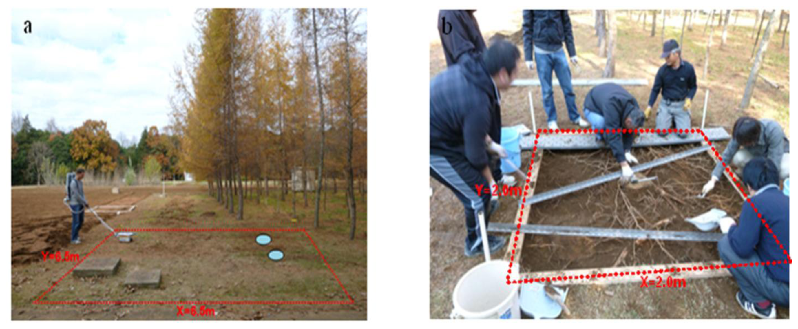
2.1. Survey Site

The field tree roots measurements were carried out at National Institute for Environment Studies in Japan [32,33]. The survey site was dominated by larch trees (Larix kaempferi L.) with 2.0 m by 3.0 m tree spacing, and covered by the common brown forest soil in Japan. The root systems of two larch trees (the average diameter at breast height (DBH) is 14 cm and tree height (H) approaches 14 m) were selected for GPR survey in a rectangular area of 6.5 m by 6.5 m. Figure 1a shows the scene of the survey site. The red dotted line shows the survey area and the two blue ellipses show the locations of the two larch trees which had been cut down beforehand. In order to evaluate soil permittivity, time-domain reflectometry (TDR) measurements were conducted at different points within the surveying area. The average of the measured relative permittivity in the near surface of soil was 18, and this meant wet soil with a volumetric water content of 32% (calculated with the equation in [34]). After the GPR measurement, one of larch trees was excavated using an archaeological method, within the area of 2.0 m by 2.0 m (shown in Figure 1b). The soil within the depth range of 10 cm was removed and all tree roots were exposed. Subsequently, the information on the exposed roots and their distributions were recorded before they were cut with a saw. This procedure was repeated until the excavation depth reached 50 cm. The collected roots were oven dried and weighed, especially the weight of coarse roots and total weight of the roots, in each 10 cm depth range, were measured.

2.2. Data Acquisition by 3D GPR

Full-resolution 3D imaging can delineate the unaliased architecture of the shallow subsurface, and high-density GPR data acquisition usually is an essential condition. Many of the previous 3D images in tree root studies are spatially aliased due to the sparse intervals between parallel profiles. Although the orientation of roots can be predicted according to their linearity, many details of root architecture have been lost. Hence, full-resolution 3D imaging will provide a promising view in tree root studies. According to the derivation in [29], the lateral intervals Δx in X direction of spatial sampling should be equal or smaller than the Nyquist sampling intervals Δx_N,

$$\mathrm{\Delta }x\le \mathrm{\Delta }{x}_N=\frac{{\lambda }_m}{4\text{sin\hspace{0.17em}}\alpha }$$

(1)

where λ_m is the wavelength in the subsurface medium and α is the main beam angle of antenna. The intervals Δy in Y direction is the same as Δx. In the near field, the beam angle usually is more than 60°, so Δx_N, approaches a quarter-wavelength in the medium.

3D GPR system integrates the commercial GPR system and a portable rotary laser positioning system (RLPS), and fuses the accurate coordinates of the moving antennas into the acquired GPR traces [28]. Briefly, a RAMAC/GPR ProEx system (MALÅ GeoScience, Malå, Sweden) was used in this measurement, and two types of shielded bow-tie antennas were employed for transmitting the ultra-wideband (UWB) impulses with center frequencies of 500 MHz and 800 MHz, respectively. The sampling rates of the system were set to 512, and the corresponding sampling intervals were 123 ps and 55 ps, respectively.

Table 1. Principle parameters of two types of antennas.

Parameters	500 MHz Shielded Antenna	800 MHz Shielded Antenna
−10 dB low limit frequency: fL	138 MHz	230 MHz
−10 dB high limit frequency: fH	591 MHz	1.280 GHz
−10 dB bandwidth: Bf	453 MHz	1.050 GHz
Center frequency: fc	364 MHz	755 MHz

shows the principal antennas parameters after the spectrum analyzing of the received waveform. Due to the dispersion effect of soil, the components of a higher frequency suffer from more serious attenuation, which certainly results in center frequency downshifting.

According to Equation (1) and Table 1, the theoretical Nyquist spatial sampling intervals can be calculated by the beam angle of 60° and the center frequency f_c, which are 6 cm for 500 MHz antenna and 3 cm for 800 MHz antenna, respectively. Therefore, in order to satisfy the condition of full-resolution 3D imaging, the interval of inlines was set to 2.5 cm, and the interval of crosslines was set to 5 cm for the measurement using the 500 MHz shielded antenna; meanwhile, the interval of inlines was set to 1.2 cm, and the interval of crosslines was set to 2.4 cm for the measurement using the 800 MHz shielded antenna. During the 3D GPR survey, one operator dragged the antennas, moving backwards and forwards, on the ground to cover the whole survey area as densely as possible. Meanwhile, the moving path of the antenna was kept straight in order to prevent voids in the acquired data in the local area.

Under the guide of RLPS, it took about two hours to complete the whole survey (261 scanning lines) using 800 MHz antenna, and one hour for 500 MHz antenna (132 scanning lines). Figure 2a,b shows the trajectories of all scanning lines recorded by the 3D GPR system, and the scanning lines using the 800 MHz antenna are obviously much denser than the 500 MHz antenna.

2.3. Data Preprocessing

After accomplishing the whole survey using 3D GPR, the acquired raw data included all A-scans, which were obtained along the moving trajectory, as shown in Figure 2, and their positioning information. Consequently, some necessary data preprocessing procedures were performed on the acquired raw data, which were listed as follow:

(a)

Regularization, which should interpolate the acquired traces (A-scans) into a regular grid using the nearest neighbor interpolation according to their accurately positioning information, finally outputs a 3D data cube;

(b)

Zero time correction, set the arrival time of the reflection from ground surface as time zero, which is an important step for migration and root localization;

(c)

Background removal, removed the strong direct wave and the coupling, and made the reflection from tree roots more obvious;

(d)

Band-pass filtering, set f_L and f_H in Table 1 as the passband limit for removing the direct current offset and suppressing high-frequency noise.

(e)

Attenuation compensation. Energy attenuation could result in the reflected amplitude decreasing rapidly, especially in this wet soil. It was very difficult to fit an attenuation curve of propagation in the field conditions. Although it is impossible to compensate for the amplitude attenuation accurately, automatic gain control (AGC) was still a practical method to be used in this measurement. The length of the sliding window, an important parameter of AGC, was set to a quarter of the sampling number.

(f)

3D migration, employed the F-K migration method to focus the reflections from the targets to the correct position beneath the surface. Wave velocity of propagation in the soil approximated to 0.071 m/ns, according to the relative permittivity measured by TDR, under the assumption that it was nearly constant in the shallow subsurface of soil.

(g)

Hilbert transform, generated the magnitude information instead of their amplitude after 3D migration, which was a necessary step for root detection and indexes extraction from the profiles.

2.4. Root Detection Procedure in 3D Data Cube

For tree root detection, an important biological feature that all of the roots of one tree extends radially from its stump should be taken into consideration. In [33], it was concluded that a good detection result was impossible by setting a simple global threshold, and a feasible idea is to search for the strong intensity of coarse root starting from the tree stump. Additionally, there was an important assumption in the 3D detection procedure that only pixels with a strong intensity, showing a linear and slender structure, could be detected as roots. Because some fine roots interlace with each other densely, and the clutter, are both shown as large area with high intensity in the 3D data cube, they could not be identified under the limited horizontal resolutions of the used GPR system. Therefore, a searching algorithm, based on threshold detection, is proposed to delineate the coarse roots, and this searching algorithm starts from the location of stump in the 3D data cube. Suppose that I = {I_m,n,k|1 ≤ m ≤ M, 1 ≤ n ≤ N, 1 ≤ k ≤ K} represents the intensity set of all pixels in 3D data cube after migration and Hilbert transform, where I_m,n,k is the intensity value of the pixel at the location (m, n, k) and m, n, k are the indexes along the X, Y, and Z (depth) directions, respectively. The detection algorithm can be divided into several steps:

(a)

Firstly, it is necessary to find the location of the tree stump in the migrated data cube, which can be expressed by I_s = {I_m,n,k|I_m,n,k ∈ I, m₁ ≤ m ≤ m₂, n₁ ≤ n ≤ n₂, 1 ≤ k ≤ K}, where [m₁, m₂] and [n₁, n₂] define the area of stump. Here, one specific value Th1 is set as the global threshold for root detection. Based on threshold detection theory, pixels in I_s whose intensity are more than Th1 will be treated as root candidates. The detection result B, related to the whole data cube, could be predefined as:

$${\text{B}}_{m,n,k}=\{\begin{array}{ll}1\hfill & if\hspace{0.17em}{I}_{m,n,k}\ge Th1,I_{m,n,k}\in {\mathbf{I}}_{\text{s}}\hfill \\ 0\hfill & if\hspace{0.17em}{I}_{m,n,k}<Th1,I_{m,n,k}\in {\mathbf{I}}_{\text{s}}\hfill \\ 0\hfill & I_{m,n,k}\in \mathbf{I}\backslash {\mathbf{I}}_{\text{s}}\hfill \end{array}$$

(2)

Then, four marginal vertical profiles are extracted from I_s: S₁ = {I_m,n,k|I_m,n,k ∈ I_s, m = m₂}, S₂ = {I_m,n,k|I_m,n,k ∈ I_s, m = m₁}, S₃ = {I_m,n,k|I_m,n,k ∈ I_s, n = n₁}, and S₄ = {I_m,n,k|I_m,n,k ∈ I_s, n = n₂}. According to this setup, the searching procedure will start from these four extracted profiles and proceed in the east, west, south, and north directions in the 3D data cube I. The Y direction in the measurement is defined as north.

(b)

The searching procedure is iterative and each root candidate in four profiles will become the start position of an iteration. For example, if the start position locates at (m₂, n, k) in S₁ and its corresponding B_m2,n,k = 1 in B, the searching procedure will start from the current pixel I_m2,n,k and go east. For the current pixel I_m2,n,k, there are five potential searching directions in its 6-connected neighborhood {I_m2,n,k}_N6 which include I_m2+1,n,k, I_m2,n−1,k, I_m2,n+1,k, I_m2,n,k−1, I_m2,n,k+1, and excludes I_m2−1,n,k, which is opposite to the search direction. Here, there is an assumption that the value of the pixel along the root is the maximum in its connected neighbourhood. Based on this, if the maximum value max [{I_m2,n,k}_N6] among these five potential pixels is more than Th1, the next search position will be determined towards the maximum value. In order to keep the search stable and effective, the values of {I_m2,n,k}_N6 are commonly obtained by the means in their 6-connected neighbourhood.

(c)

After determining the searching direction, the tree root candidate pixels need to be detected in the 26-connected neighbourhood {I_m2,n,k}_N26 of the current pixel. It is assumed that the profile of a root in GPR data is made up of several pixels, where the size of one pixel only represents Δx × Δy × Δz (length × width × depth). Therefore, based on the intensity of the current pixel I_m2,n,k, any pixels in {I_m2,n,k}_N26 whose intensities are more than 0.707I_m2,n,k (−3 dB) will be detected as root candidates, and their corresponding positions in detection result B will be set to 1.

(d)

In case there are several weak reflections, resulting from the local sparse spatial sampling, a lower threshold Th2 (Th2 < Th1) is introduced in the searching procedure. If Th1 is the only threshold, it is inevitable that the detected root will be cracked. Here, there is an assumption that the section with weak intensity is local and infrequent. Therefore, when max [{I_m2,n,k}_N6] is less than Th1, it is necessary to enlarge the search range two or three pixels forward along the searching direction. Then, if one pixel with an intensity of more than Th1 can be found, the search will continue. Otherwise, the current searching process will end, and another search will restart from the next candidate position (m₂, n+1, k) in S₁ whose corresponding value in B is 1. It is a special case that detection of the weak reflection is based on Th2, thus, the cracked sections in the detection result will be connected.

(e)

Steps b–d will repeat until the searching end condition has been met or the current position reaches the boundary of the data cube. Then, another searching process will restart from the next candidate position in S₁ whose corresponding value in B is 1. When all search processes starting from S₁ to S₄ are complete, the 3D searching procedure will terminate.

After the 3D detection procedure, common morphological processing methods are employed to enhance the visualization of the 3D detection result, which include morphological size filtering, open and close operations, etc. [35].

2.5. Indexes Extraction from GPR Data for Biomass Estimation

After data preprocessing of 3D GPR data cube described in Section 2.3, some GPR indexes can be extracted for root biomass estimation and root diameter estimation. Most of them have been introduced in previous studies, which include pixels within threshold range, high amplitude area, time interval between two zero crossings, and so on. Different from the other indexes, pixels within threshold range is an index of the reflected intensity which can be extracted not only in 2D GPR profiles but also in a 3D GPR cube. In addition, a proper threshold needs to be set beforehand to count the pixels within threshold range to estimate root biomass. However, the estimating performance of this index depends on many factors (e.g., antenna frequency, soil properties, root species, and so on), which is site-specific [10]. High amplitude area and time intervals between two zero crossings are extracted from the reflected waveform before implementing Hilbert transform [10,17], which are defined in Figure 3a,b. In addition to these common indexes, this paper proposed a new index to estimate the root diameter directly named by “magnitude width Δw” (Figure 3c). As its name implies, this index should be extracted on the magnitude curve after Hilbert transform. Beside the pixels within threshold range, extraction of the other three indexes has to be performed, based on the results of root detection. Otherwise, it can not select true waveforms from the great deal of root reflections and clutter in 3D data cube.

2.6. Construction of Biomass Estimation Models

After GPR indexes extraction, the relationship between these extracted indexes and true values of biomass and diameter needs to be fitted by linear regression models and non-linear regression models. The reliability of regression models depends on whether the soil condition is controlled or it has enough extracted root samples. When the detected root samples in GPR data are relatively less, reliable complicated regression models are hard to be constructed, and constructing a simple linear regression model is much more feasible.

The correlation between the extracted GPR indexes and the true root biomass (root diameter) commonly is calculated by the Pearson correlation coefficient (r) [17]. The calculation formula of r is:

$$r=\frac{{\displaystyle \sum _{i=1}^N}(x_i-\overline{x})(y_i-\overline{y})}{\sqrt{{\displaystyle \sum _{i=1}^N}{\left(x_i-\overline{x}\right)}^2\sum _{i=1}^N{\left(y_i-\overline{y}\right)}^2}}$$

(3)

where x_i is the extracted index for the i-th root sample, χ̄ denotes the mean of x_i, y_i is the true root biomass or diameter for the i-th root sample, ȳ denotes the mean of y_i, and N is the number of the root samples detected in 3D data cube. Coefficient r ranges from −1 to 1. An absolute value of 1 implies that the extracted GPR indexes and the true root biomass have a perfectly linear relationship, and a value of 0 implies no correlation between them.

3. Results and Discussion

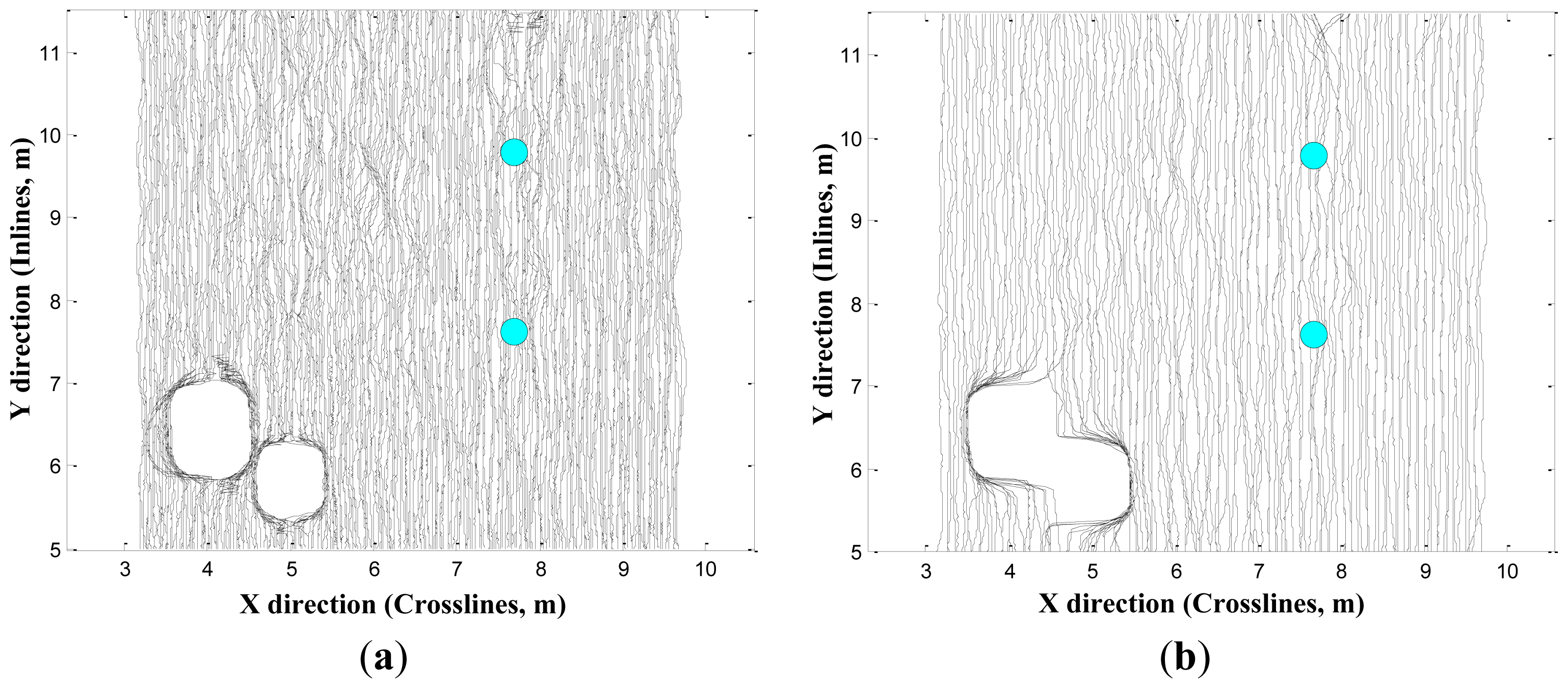
3.1. 3D Migrated Results of GPR Data Cube

Figure 4 shows the horizontal slices after 3D migration at three different depths (0.1 m, 0.2 m, and 0.3 m) using the 500 MHz and 800 MHz antennas, respectively. More detailed distributions of roots in the migration results are shown using the 800 MHz antenna than the 500 MHz antenna. An important factor is the imaging resolution of the GPR system, which includes vertical resolution Δ_V and horizontal resolution Δ_H. The typical calculation equations to estimate Δ_V and Δ_H [36] are:

$${\mathrm{\Delta }}_V=\frac{v_m}{4B}$$

(4)

$${\mathrm{\Delta }}_H=\sqrt{\frac{{\lambda }_m^2}{4}+z{\lambda }_m}$$

(5)

where ν_m and λ_m are the propagating velocity and wavelength of the transmitted impulse in the medium respectively, B is the bandwidth of −3 dB of the transmitted impulse, and z is the depth beneath the antenna. According to Equations (4) and (5), the relative permittivity of the medium is also a key factor for the imaging resolution. However, the dielectric properties of the medium (including relative permittivity ɛ_m and conductivity σ_m) always oppose each other because soil with high permittivity usually has a high conductivity, which induces a shallow penetrating depth. In this measurement, the theoretical vertical resolution for the 800 MHz bow-tie antenna Δ_V ≈ 5 cm, and the horizontal resolution Δ_H ≈ 10cm at a 0.10 m depth, which have better resolution capabilities than the 500 MHz antenna (Δ_V ≈ 6 cm and Δ_H ≈ 14 cm at a 0.1 m depth).

As shown by the white arrows in Figure 4, there are some structures imaged with both antennas, which extend from the tree stumps (black dashed circles). If the different depth slices of the migration results could be displayed as frames of an animation, it would be much clearer to see the anomalies reflected from the roots. From the migration results, most of the reflections from roots locate in the shallow soil (depth ≤ 0.30 m), such as Figure 3b,d. As the spatial distribution of the roots is not planar, the amplitude of reflection from one root showed varied brightness in the same depth slice. In order to compare the migrated results and the true tree root distribution, one of the larch trees (at x = 4.5 m, y = 3.1 m) was excavated, and the true root structures at the different depths are shown in Figure 5a–c. Meanwhile, the corresponding data cube of the excavated area is extracted from the whole migrated cube of the 800 MHz antenna. The corresponding migrated horizontal slices at three different depths are shown in Figure 5d–f.

Different from optimal conditions for measuring tree roots, such as buried roots in a sandpit, the distributions of roots in the field are much more complicated. In Figure 5a,b, except for coarse roots labeled by arrows and numbers, there are a lot of crossings fine roots of which diameters are less than 10 mm. According to the theoretical horizontal resolution at 0.10 m depth, if the interval between two roots is more than 10 cm, then they can be recognized individually in the GPR profiles. Unfortunately, the areas (labeled by Roman numerals I, II, and III in Figure 5) filled with fine roots produce signals with the strong amplitude and show the same bright blocks as the clutter, which are generated mainly by the heterogeneous soil. Hence, it is difficult to discriminate the fine roots by GPR in the field. From the migrated slices, the edge area of the tree stump usually shows strong back scattering due to the reflections from the edge of the stump. The reflections from coarse roots can be detected from the migrated slices depending on their orientations and surroundings. Because of the typical linearly-polarized feature of the bow-tie antenna, if the orientation of roots is parallel with the long axes of the bow-tie antenna, reflections from the roots will be the strongest, such as with root 1 and 2 in Figure 5a. Otherwise, the reflections will weaken, such as with root 10 and 11 (Figure 5b) [23,27]. There are other reasons for difficultly discriminating coarse roots from dense areas with strong amplitudes. For example, if many fine roots cover the deeper coarse root (roots 5, 9, 13, and 14 in Figure 5a,b), it is hard to detect the coarse root. If two coarse roots are close to each other and the interval between them is less than the theoretical horizontal and vertical resolutions (roots 3, 4, and 7), the reflections will include both of them.

According to characteristics analysis of roots in the migrated cube by 3D GPR, it is feasible to detect the coarse roots in 3D migrated data cube. Furthermore, in order to delineate the distributions of the coarse roots, it is inevitable to detect them in a 3D space and not only in the horizontal slices. An important fact is that these reflections all extend radially from the tree stump, which is key to differentiate the roots from the clutter.

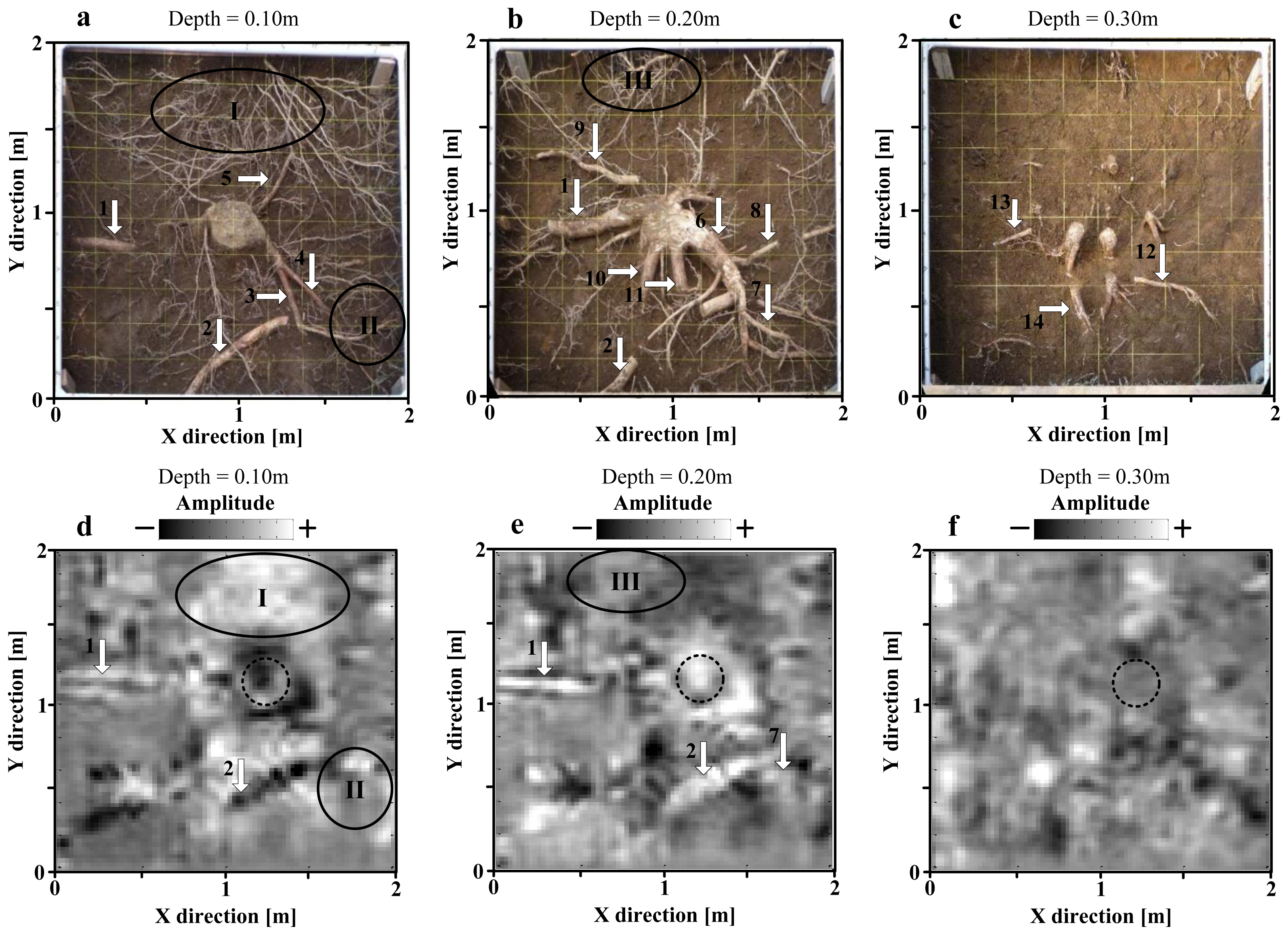
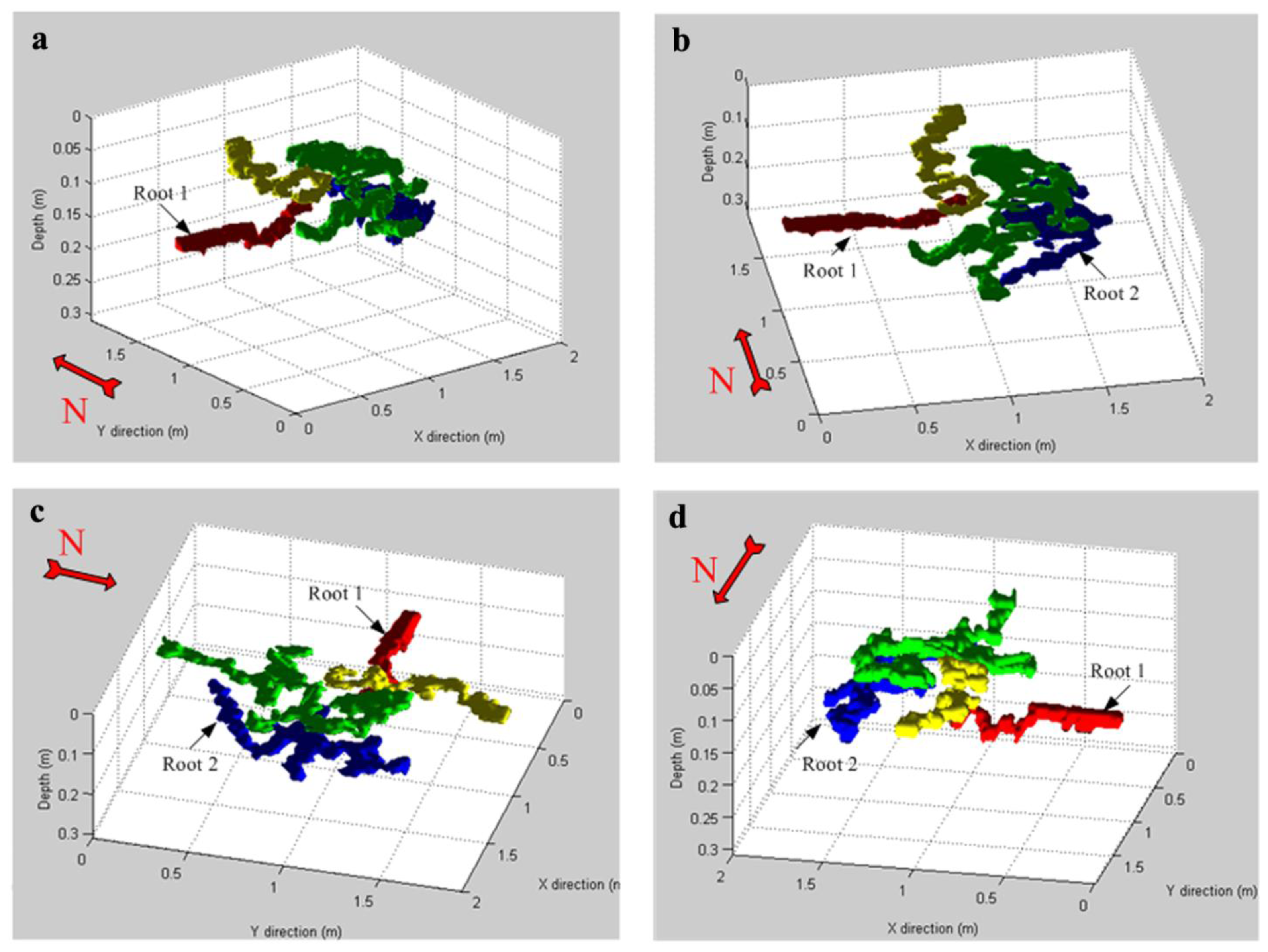
3.2. Detection Result of Coarse Roots in 3D Data Cube

The normalized data cube after migration using the 800 MHz antenna is selected to verify the feasibility and effectiveness of the proposed detection procedure, and its size is limited to the excavated area, which is shown in Figure 5. Meanwhile, considering that the tree roots mostly locate above 0.30 m depth and the strong attenuation of the transmitting signal in the soil, only part of the cube above 0.30 m depth is used for detection. As mentioned in the 3D detection procedure, the area of the tree stump is defined from 1.0 m to 1.45 m in the X direction, and from 0.80 m to 1.24 m in the Y direction according to its actual location [33].

In this 3D detection procedure, the value of Th1 is set to 0.65 and the value of Th2 is 0.55. According to the detection procedure, each pixel in the profiles S₁–S₄ whose intensity is more than 0.65 serves as the starting position of each iteration. After accomplishing the 3D detection procedure, morphological size filtering will remove the 6-connected objects in 3D data cube whose sizes are smaller than 50 pixels. The final 3D detection result is drawn by the volume visualization functions in Matlab. The 3D graphic of the result is shown from four different viewpoints in Figure 6. From the detection results, tree root 1, which is labeled in red, and tree root 2, which is labeled in blue can be detected correctly, and their distributions conform to the true scene shown in Figure 5. There are also false alarms (in green and yellow) in the detection results, which actually are some clutter-like roots. However, this detection method can remove the influence of strong reflections in a large area caused by the clustering of fine roots and clutter. In the field data set, usually there is not a strong contrast between the reflections from coarse roots and clutter, as seen in the migrated slices. In addition, it is almost impossible to detect each section of coarse roots slice by slice in the data cube. Nevertheless, the spatial distribution characteristic of coarse roots (extend from the stump) provides a good basis for searching the extension of root in the 3D data space, and actually works. Since the intense distributions of coarse roots and fine roots locate closely around the tree stump, it is inevitable that some clutter is detected as roots and some coarse roots are undetected. Of course, the resolutions of the GPR system also limit the detection probability of two close roots.

3.3. Root Biomass Estimation from GPR Data

In this case, based on the 3D detection result, some samples of the detected root 1 and 2 can be extracted from the sequential vertical profiles with the same width, of seven pixels, along the Y direction in the migrated cube. The sample sizes of root 1 and 2 are 20 and 17, respectively, representing for 48 cm and 40.4 cm long in X direction (each pixel represents for 2.4 cm × 2.4 cm in X direction and Y direction). Figure 7a,c show the migrated profiles in which all samples are spliced together in the same profile, meanwhile, Figure 7b,d show the corresponding normalized magnitude profiles after Hilbert transform. With this measurement setup, it is feasible to estimate the total biomass of roots using the intensity indexes (pixels within threshold range) extracted from the GPR data. The key of this method is to set an appropriate overall threshold to discriminate roots from clutter in the GPR data as much as possible. As previously mentioned [16,19], a linear regression model can estimate the biomass well using pixels within threshold range. Therefore, the extracted intensity index of root 1 and 2 and their true root biomass can be used to build a linear regression model. The dry weight of the collected root 1 was 104 g and 25 cm long, and the collected root 2 was 117.4 g in dry weight, 47 cm long. Comparing the recorded root distributions with the coordinates of the migrated data cube, sample 5–15 of root 1 (representing for Figure 7b) and sample 1–17 of root 2 (Figure 7d) were selected to calculate the corresponding total pixels numbers. Meanwhile, a threshold of 0.165 was used because it provides a good balance between clutter reduction and the discrimination of roots in the GPR data cube. The cumulative pixel sizes of root 1 and root 2 in the GPR data with an intensity of more than the threshold are 3023 and 3422, respectively. Hence, the linear regression model was built with the following equation:

$$(\text{Estimated\hspace{0.17em}total\hspace{0.17em}root\hspace{0.17em}biomass})=0.0336\times (\text{Pixel\hspace{0.17em}numbers\hspace{0.17em}within\hspace{0.17em}threshold\hspace{0.17em}range})+2.42$$

(6)

The dry weight of all roots collected in the 0–10 cm, 10–20 cm, 20–30 cm, 30–40 cm and 40–50 cm excavation ranges were tallied. According to Equation (6), the estimated total root biomass related to five different depth ranges can be roughly calculated by accumulating total pixels numbers whose intensity exceed the overall threshold.

Table 2. Comparison of the estimated results of biomass with Ground Penetrating Radar (GPR) and the measured actual biomass at each 10 cm depth range.

Depth Range (cm)		0–10	10–20	20–30	30–40	40–50	0–50
Estimated Weightwith GPR (g)		2404.8	4101.6	2403.2	1960.2	1293.8	12,163.6
Dry Weight of All Roots (g) (*Error)	Including Tree Stump	5697(−55.8%)	9909.8(−58.6%)	1937.4(+24%)	2251.4(−12.9%)	1468.7(−11.9%)	21,264.3(−42.8%)
	Excluding Tree Stump	1744.5(+37.9%)	3664.6(+11.9%)	1937.4(+24%)	2251.4(−12.9%)	1468.7(−11.9%)	11,066.6(+9.9%)

^*The signs of error (“+” and “−” indicate over-estimation and the under-estimation respectively.

lists the true and estimated values of root biomass in five different depth ranges. Because of weak reflections from the taproot when the antenna is moving over the tree stump, the weight of the tree stump was extracted and considered separately. If the biomass of the tree stump is taken into account, it will result in serious under-estimation of the total biomass. Excluding the biomass of the taproot, the estimated total root biomass approaches the actual mass of the roots well, within the 10% error range (including all coarse roots and fine roots). In spite of this, the total biomass of the roots above the 30 cm depth is over-estimated because of the existence of clutter and fine roots. Meanwhile, the total biomass of roots within the 30–50 cm depth range is under-estimated because of energy attenuation of the electromagnetic wave in the soil and interference of the shallow roots. This estimation method could still roughly estimate the total biomass of all roots beneath the survey area.

3.4. Root Diameter Estimation from GPR Data

Root diameter estimation from GPR indexes is feasible only to estimates the diameter of the detected coarse roots in the migrated data cube. Those undetected roots usually can not show the shape of root in the 3D data cube, thus, it is not very convincing to link the GPR indexes with the root diameters. In this paper, all samples of the detected root 1 and root 2 (Figure 7), combining their true root diameters are selected for studying their correlations. These GPR indexes, including pixels within threshold range, high amplitude area (dB × ns), time intervals (ΔT₁ − ΔT₄, ns) between zero-crossings, and the proposed magnitude width Δw, are selected for comparing the correlations with the true diameters. The results of the evaluated correlation coefficients are listed in Table 2. Overall, the GPR indexes related to the intensity of pixels (such as pixels within threshold range and high amplitude area) have a slightly weaker correlation with root diameter than the indexes directly extracted from the waveform, because it is hard to ensure the same reflected amplitude in each sample due to non-uniform spatial sampling and heterogeneous soil in field measurement. Additionally, the overall correlations calculated by the samples of root 1 are better than root 2. Due to the lack of sufficient samples, it is difficult to construct an estimation model of root diameter as Cui et al. did [17]. Among the related GPR indexes extracted from the radar profiles (in

Table 3. Correlation coefficient (r) between the true root diameter and the extracted GPR indexes from root 1 and 2 samples.

Root Samples (Size: n)	Pixels within Threshold Range	High Amplitude Area	Time Interval ΔT3	Total Time Interval ΔT = ΔT1 + ΔT2 + ΔT3 + ΔT4	Magnitude Width Δw
Root 1 (20)	r = 0.5189	r = 0.5630	r = 0.7012	r = 0.6613	r = 0.7889
	p = 0.019	p = 0.005	p < 0.001	p < 0.001	p < 0.001
Root 2 (17)	r = 0.1751	r = 0.1560	r = 0.6734	r = 0.6098	r = 0.6874
	p = 0.397	p = 0.451	p < 0.001	p = 0.002	p < 0.001

), time interval ΔT₃ and magnitude width Δw have better correlation with the actual diameter than others. Compared to time interval ΔT₃, the magnitude width Δw (cm) provides a direct measurement of root diameter with more apparent physical meaning. Furthermore, the magnitude width is only determined by the −3 dB positions of the intensity value at the local peak, which still works with the weak reflections of the detected roots (as shown in Figure 3c).

Thus, it is reasonable to use the magnitude width Δw for estimating the root diameter directly. However, the intersection angle (θ) between the survey lines and the orientation of roots affects the model of diameter estimation. According to the analysis in [23], the hyperbola reflected from the roots in GPR profile has a narrow width under the condition of an intersection angle of 90°. When the intersection angle is less than 90°, the hyperbolas will become wider and relatively flat. Hence, the root diameter (D_est) can be estimated by the following equation:

$$D_{est}=\mathrm{\Delta }w\times \text{sin\hspace{0.17em}}\theta$$

(7)

The detection results of tree roots show that the intersection angles of root 1 and root 2 with the scanning lines approaches to 90° and 60° respectively, which also can be verified by the scene after root excavation (Figure 5a). Based on the samples in Figure 7b,d, the evaluated magnitude width Δw and the estimated average diameters of roots 1 and 2 are listed in

Table 4. Diameter estimated results from GPR data.

Root Samples (Size: n)	Average Magnitude Width Δw (cm)	Estimated Average Diameter (cm)	True Average Diameter (cm)	Error
Root 1 (20)	5.3	5.3	6.1	13%
Root 2 (17)	5.5	4.8	5.7	16%

. From the estimation results, the magnitude width Δw can be regarded as the estimated root diameter, which approaches its true value. Although the estimation errors are usually larger than those which were carried out under optimal conditions, overall, this approach can still provide an alternative method for the rough diameter estimation of tree root in field measurement.

4. Conclusions

With the aid of the advanced 3D Ground Penetrating Radar (3D GPR) system, this is the first time to obtain a full-resolution 3D image of a larch tree root system and to view the spatial distribution of coarse roots in the field. According to the distribution characteristics of tree root in the migrated cube, a searching detection algorithm is proposed to detect coarse roots starting from the tree stump that eliminates the influence of strong clutter as much as possible. The excavation result of one tree root verifies that two coarse roots can be still delineated in the detection result correctly in spite of other two false roots detected. Based on the detection result, the samples of the detected coarse roots were extracted from GPR data cube for root biomass estimation. Firstly, a simple linear regression model correlated the GPR index (pixels within threshold range) and dry weight of root was built for total root biomass estimation at each 10 cm depth range. The estimation result shows an error range from −13% to +38% at the different depths and a total error of +10% without considering the biomass of tree stump, where the signs of error (“+” and “−”) indicate over-estimation and the under-estimation respectively. Although it is difficult to estimate the root biomass accurately using the GPR indexes related with the pixel intensity, it still provides a simple and feasible method for total biomass estimation in the field at least. Then, a new GPR index called “magnitude width” is proposed in this paper which is extracted from the normalized magnitude profile after the migration and Hilbert transform. The calculations of Pearson correlation coefficient show that the proposed magnitude width has a better correlation with the root diameter in the field measurement, comparing with other common GPR indexes. Furthermore, the proposed magnitude width provides a direct estimation of root diameter, and the detected samples from GPR profiles verify the estimated root diameter with error around 15%.

This is only a case study on the coarse root detection and biomass estimation, based on the 3D GPR data acquired by a novel 3D GPR system. Although it is impossible to totally detect and estimate the entire root system using GPR, it still demonstrates the potentials of a 3D GPR system as an effective and convenient tool, which can be used in future works in tree root studies.

References

1. Daniels, D.J. Ground Penetrating Radar, 2nd ed; Institution of Engineering and Technology: London, UK, 2004. [Google Scholar]
2. Harry, M.J. Ground Penetrating Radar: Theory and Application, 1st ed; Elsevier Science: Amsterdam, The Netherlands, 2009. [Google Scholar]
3. Sato, M.; Yokota, Y.; Takahashi, K.; Grasmueck, M. Landmine detection by 3DGPR system. Proc. SPIE 2012, 8357, 23–27. [Google Scholar]
4. Youn, H.; Chen, C. Neural Detection for Buried Pipes Using Fully-Polarimetric Ground Penetrating Radar System. Proceedings of the 10th International Conference on Ground Penetrating Radar, Delft, The Netherlands, 21–24 June 2004; pp. 231–234.
5. Hruska, J.; Cermák, J.; Sustek, S. Mapping tree root systems with ground-penetrating radar. Tree Physiol 1999, 19, 125–130. [Google Scholar]
6. Moran, C.J.; Pierret, A.; Stevenson, A.W. X-ray absorption and phase contrast imaging to study the interplay between plant roots and soil structure. Plant Soil 2000, 223, 99–115. [Google Scholar]
7. Butnor, J.R.; Johnsen, K.H.; Wikström, P.; Lundmark, T.; Linder, S. Imaging Tree Roots with Borehole Radar. Proceedings of the 11th International Conference on Ground Penetrating Radar, Columbus, OH, USA, 19–22 June 2006; pp. 1–8.
8. Amato, M.; Basso, B.; Celano, G.; Bitella, G.; Morelli, G.; Rossi, R. In situ detection of tree root distribution and biomass by multi-electrode resistivity imaging. Tree Physiol 2008, 28, 1441–1448. [Google Scholar]
9. Brunner, I.; Godbold, D.L. Tree roots in a changing world. J. For. Res 2007, 12, 78–82. [Google Scholar]
10. Guo, L.; Chen, J.; Cui, X.; Fan, B.; Lin, H. Application of ground penetrating radar for coarse root detection and quantification: A review. Plant Soil 2013, 362, 1–23. [Google Scholar]
11. Wielopolski, L.; Hendrey, G.; Daniels, J.; McGuigan, M. Imaging Tree Root Systems in situ. Proceedings of the 8th International Conference on Ground Penetrating Radar, Gold Coast, Australia, 27 April 2000; pp. 642–646.
12. Zonone, T.; Morelli, G.; Teobaldelli, M.; Fischanger, F.; Matteucci, M.; Sordini, M.; Armani, A.; Ferre, C.; Chiti, T.; Seufert, G. Preliminary use of ground-penetrating radar and electrical resistivity tomography to study tree roots in pine forests and poplar plantations. Funct. Plant Biol 2008, 35, 1047–1058. [Google Scholar]
13. Leucci, G. The use of three geophysical methods for 3D images of total root volume of soil in urban environments. Explor. Geophys 2010, 41, 268–278. [Google Scholar]
14. Hirano, Y.; Dannoura, M.; Aono, K.; Igarashi, T.; Ishii, M.; Yamase, K.; Makita, N.; Kanazawa, Y. Limiting factors in the detection of tree roots using ground-penetrating radar. Plant Soil 2009, 319, 15–24. [Google Scholar]
15. Butnor, J.R.; Doolittle, J.A.; Kress, L.; Cohen, S.; Johnson, K.H. Use of ground-penetrating radar to study tree roots in the southeastern United States. Tree Physiol 2001, 21, 1269–1278. [Google Scholar]
16. Butnor, J.R.; Doolittle, J.A.; Johnson, K.H.; Samuelson, L.; Stokes, T.; Kress, L. Utility of ground-penetrating radar as a root biomass survey tool in forest systems. Soil Sci. Soc. Am. J 2003, 67, 1607–1615. [Google Scholar]
17. Cui, X.; Guo, L.; Chen, J.; Chen, X.; Zhu, X. Estimating tree-root biomass in different depths using ground-penetrating radar: Evidence from a controlled experiment. IEEE Trans. Geosci. Remote Sens 2013, 51, 3410–3423. [Google Scholar]
18. Cui, X.; Chen, J.; Shen, J.; Cao, X.; Chen, X.; Zhu, X. Modelling tree root diameter and biomass by ground-penetrating radar. Sci. China Earth Sci 2011, 54, 711–719. [Google Scholar]
19. Dannoura, M.; Hirano, Y.; Igarashi, T.; Ishii, M.; Aono, K.; Yamase, K.; Kanazawa, Y. Detection of Cryptomeria japonica roots with ground penetrating radar. Plant Biosyst 2008, 142, 375–380. [Google Scholar]
20. Barton, C.V.M.; Montagu, K.D. Detection of tree roots and determination of root diameters by ground penetrating radar under optimal conditions. Tree Physiol 2004, 24, 1323–1331. [Google Scholar]
21. Hirano, Y.; Yamamoto, R.; Dannoura, M.; Aono, K.; Igarashi, T.; Ishii, M.; Yamase, K.; Makita, N.; Kanazawa, Y. Detection frequency of Pinus thunbergii roots by ground-penetrating radar is related to root biomass. Plant Soil 2012, 360, 363–373. [Google Scholar]
22. Guo, L.; Lin, H.; Fan, B.; Cui, X.; Chen, J. Impact of root water content on root biomass estimation using ground penetrating radar: Evidence from forward simulations and field controlled experiments. Plant Soil 2013, 371, 503–520. [Google Scholar]
23. Tanikawa, T.; Hirano, Y.; Dannoura, M.; Yamase, K.; Aono, K.; Ishii, M.; Igarashi, T.; Ikeno, H.; Kanazawa, Y. Root orientation can affect detection accuracy of ground-penetrating radar. Plant Soil 2013, 373, 317–327. [Google Scholar]
24. Raz-Yaseef, N.; Koteen, L.; Baldocchi, D.D. Coarse root distribution of a semi-arid oak savanna estimated with ground penetrating radar. J. Geophys. Res 2013, 118, 135–147. [Google Scholar]
25. Isaac, M.E.; Anglaaere, L.C.N. An in situ approach to detect tree root ecology: Linking ground-penetrating radar imaging to isotope-derived water acquisition zones. Ecol. Evol 2013, 3, 1330–1339. [Google Scholar]
26. Isaac, M.E.; Anglaaere, L.C.N.; Borden, K.; Adu-Bredu, S. Intraspecific root plasticity in agroforestry systems across edaphic conditions. Agric. Ecosyst. Environ 2014, 185, 16–23. [Google Scholar]
27. Radzevicius, S.J.; Daniels, J.J. Ground penetrating radar polarization and scattering from cylinders. J. Appl. Geophys 2000, 45, 111–125. [Google Scholar]
28. Grasmueck, M.; Viggiano, D.A. Integration of ground-penetrating radar and laser position sensors for real-time 3-D data fusion. IEEE Trans. Geosci. Remote Sens 2007, 45, 130–137. [Google Scholar]
29. Grasmueck, M.; Weger, R.; Horstmeyer, H. Full-resolution 3D GPR imaging. Geophysics 2005, 70, K12–K19. [Google Scholar]
30. Böniger, U.; Tronicke, J. On the potential of kinematic GPR surveying using a self-tracking total station: Evaluating system crosstalk and latency. IEEE Trans. Geosci. Remote Sens 2010, 48, 3792–3798. [Google Scholar]
31. Böniger, U.; Tronicke, J. Improving the interpretability of 3D GPR data using target-specific attributes: Application to tomb detection. J. Archaeol. Sci 2010, 37, 672–679. [Google Scholar]
32. Yokota, Y.; Matsumoto, M.; Gaber, A.; Grasmueck, M.; Sato, M. Estimation of Biomass of Tree Roots by GPR with High Accuracy Positioning System. Proceedings of the IEEE International Geoscience and Remote Sensing Symposium 2011, Vancouver, BC, Canada, 24–29 July 2011; pp. 190–193.
33. Zhu, S.; Su, Y.; Sato, M. Detection of Tree Roots and Root Biomass Estimation based on Ground Penetrating Radar with High Accuracy Positioning System. Proceedings of the IET International Radar Conference, Xi’an, China, 14–16 April 2013; pp. 1–5.
34. Bano, M. Modelling of GPR waves for lossy media obeying a complex power law of frequency for dielectric permittivity. Geophys. Prospect 2004, 52, 11–26. [Google Scholar]
35. Gonzalez, R.C.; Woods, R.E.; Eddins, S.L. Digital Image Processing Using Matlab, 2nd ed; Prentice Hall: Upper Saddle River, NJ, USA, 2004. [Google Scholar]
36. Rial, F.I.; Pereira, M.; Lorenzo, H.; Arias, P.; Novo, A. Resolution of GPR bowtie antennas: An experimental approach. J. Appl. Geophys 2009, 67, 367–373. [Google Scholar]
Figure 1. (a) Surveying scene of larch trees using 3D GPR, the red dotted lines show the survey area and the blue circles shows the locations of the larch tree stumps. (b) Excavating scene of one larch tree root, the red dotted lines show the excavation area.
Remotesensing 06 05754f1
Figure 2. Moving trajectories of antennas recorded by the 3D GPR system, and blue circles show the locations of the tree stumps. (a) 800 MHz shielded antenna; (b) 500 MHz shielded antenna.
Remotesensing 06 05754f2
Figure 3. Schematic illustration of the extracted GPR indexes: (a) A migrated profile along a scanning line perpendicular with the root orientation. Point P locates at the peak position of the waveform right above the root. One vertical curve (indicated by solid line, at y = 1.13 m) and one horizontal curve (indicated by dashed line, at depth = 0.138 m) passing through peak P are extracted for subsequent analysis; (b) Definitions of high amplitude area and different time intervals between zero crossings are indicated based on the extracted vertical waveform; (c) Magnitude width Δw of root is defined as the width (cm) between the −3 dB positions below the peak P in the extracted horizontal magnitude curve after Hilbert transform.
Remotesensing 06 05754f3
Figure 4. Different horizontal slices extracted from the 3D migrated cube at the different depths. (a,b) Migrated slices at 10 cm depth using the 500 MHz and 800 MHz antennas, respectively; (c,d) Migrated slices at 20 cm depth using the 500 MHz and 800 MHz antennas, respectively; (e,f) Migrated slices at 30 cm depth using the 500 MHz and 800 MHz antennas, respectively. White arrows indicate the reflections from the roots in the migrated data set, and black dotted circles show the locations of the tree stumps.
Remotesensing 06 05754f4
Figure 5. (ac) True distribution scenes of one larch roots in 2.0 m × 2.0 m area, and each yellow grid represents the 20 cm × 20 cm area. After excavation at 10 cm depth each time, the exposed roots are cut off and their diameters and weights were measured separately. (df) Migrated slices extracted from the data cube corresponding to the depths of (a–c).
Remotesensing 06 05754f5
Figure 6. (ad) Visualization of 3D detection results of the tree root using Matlab in different viewpoints, red arrows indicate north.
Remotesensing 06 05754f6
Figure 7. Spliced GPR profiles of root 1 and 2 samples extracted along Y direction from the migrated data cube. The serial number of abscissa represents each root sample which has a same width of 7 pixels (16.8 cm). (a) Amplitude profile of 20 samples all extracted from root 1; (b) Magnitude profile of the samples from root 1 after Hilbert transform; (c) Amplitude profile of 17 samples all extracted from root 2; (d) Magnitude profile of the samples from root 2 after Hilbert transform.
Remotesensing 06 05754f7