TecLines: A MATLAB-Based Toolbox for Tectonic Lineament Analysis from Satellite Images and DEMs, Part 1: Line Segment Detection and Extraction


Abstract
:1. Introduction
2. Data
2.1. Synthetic Dataset
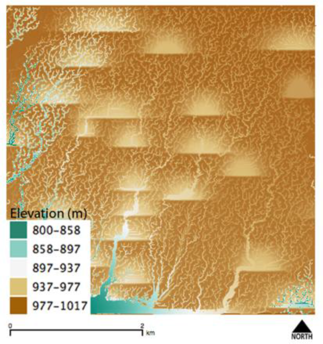
2.2. Real Dataset
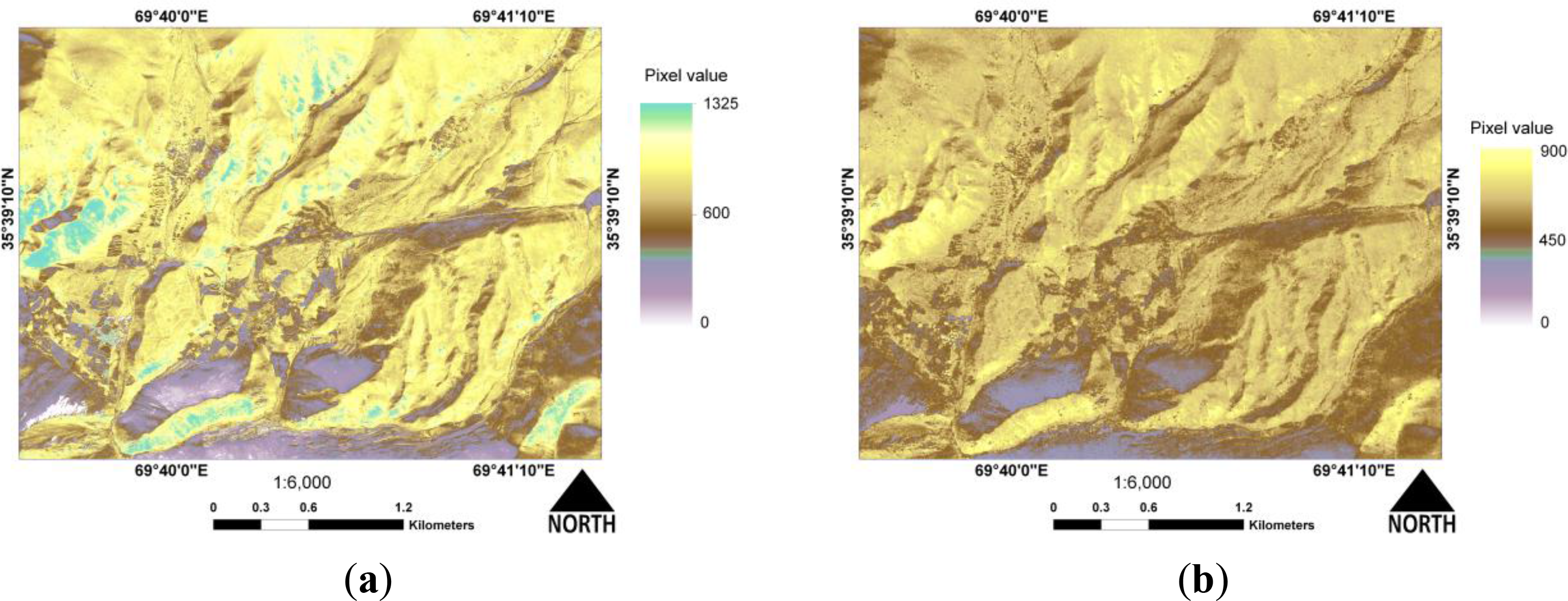
Study Area and Data
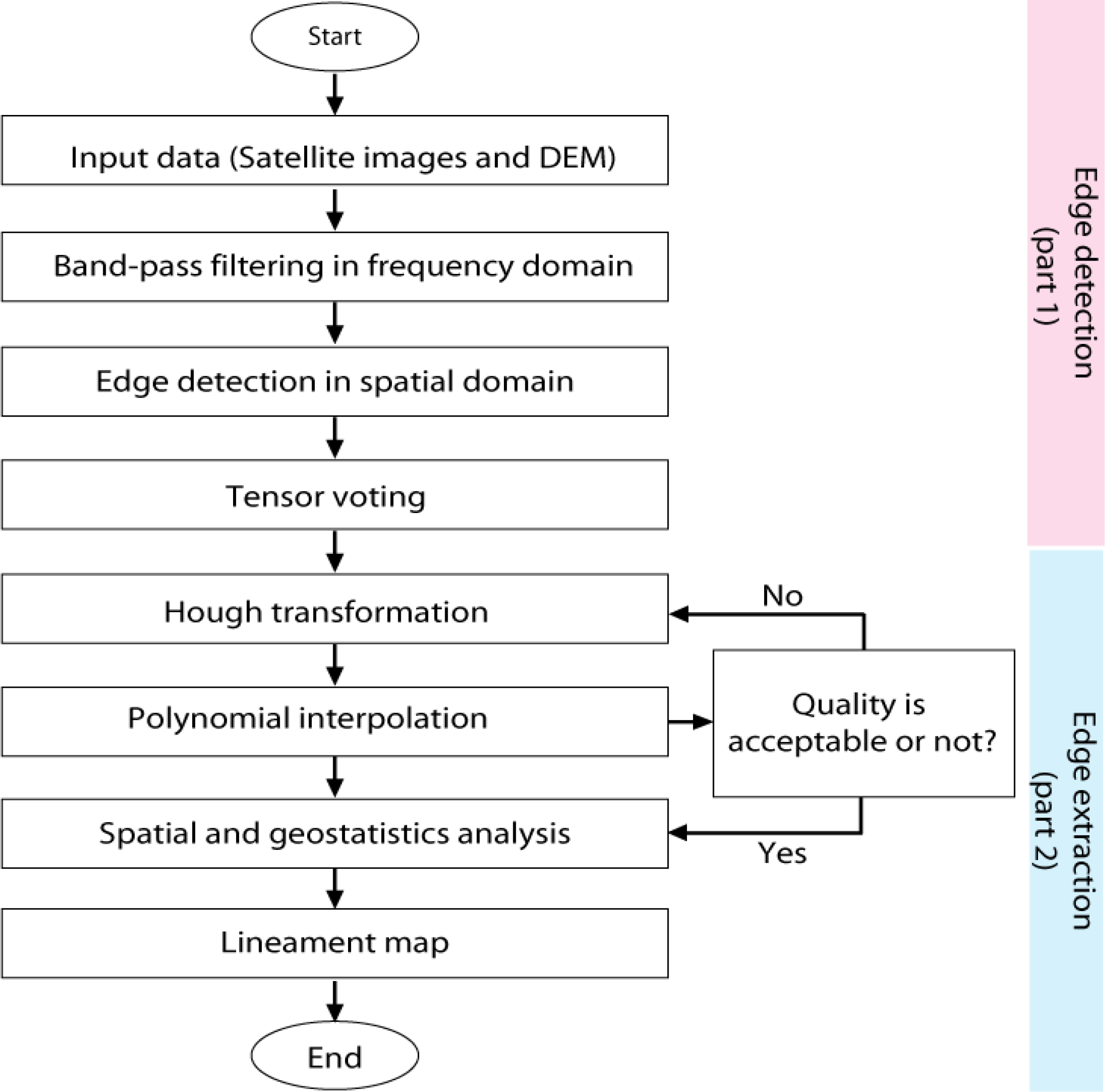
3. Methodology
3.1. Frequency Domain Filtering
3.2. Spatial Domain Filtering
3.3. Morphological Image Processing
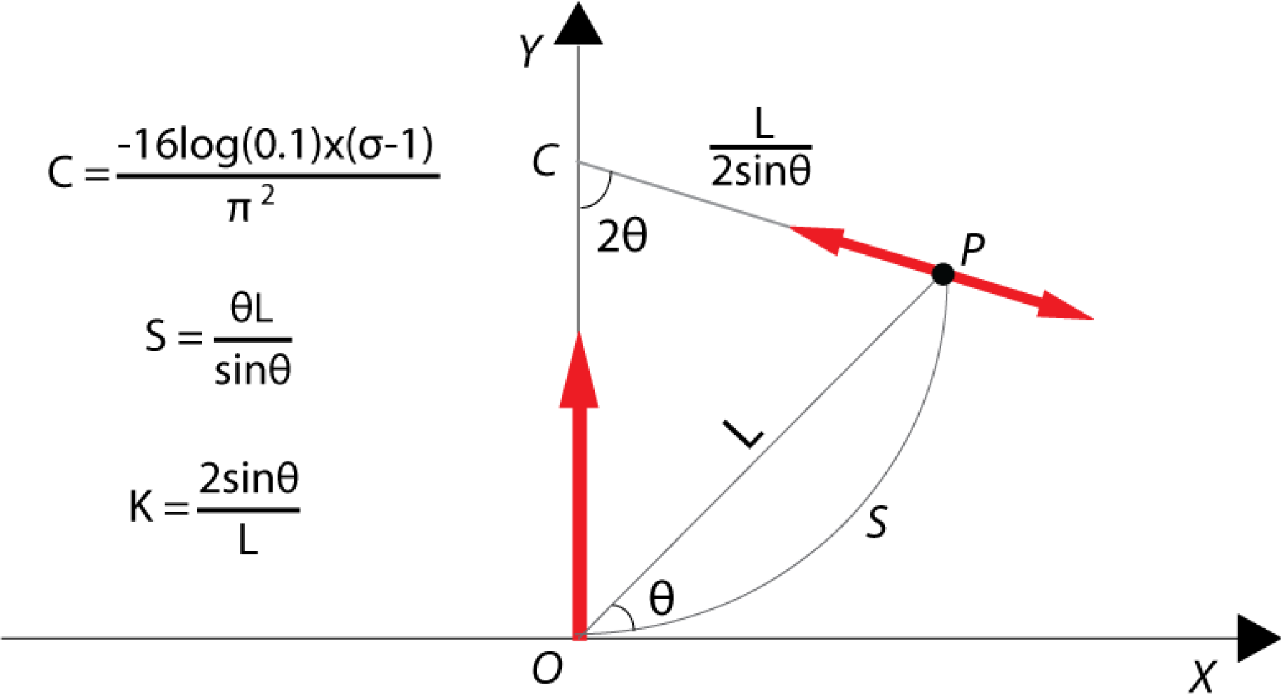
3.4. Tensor Voting Framework
3.5. Accuracy Measurements
4. Testing and Evaluating TecLines
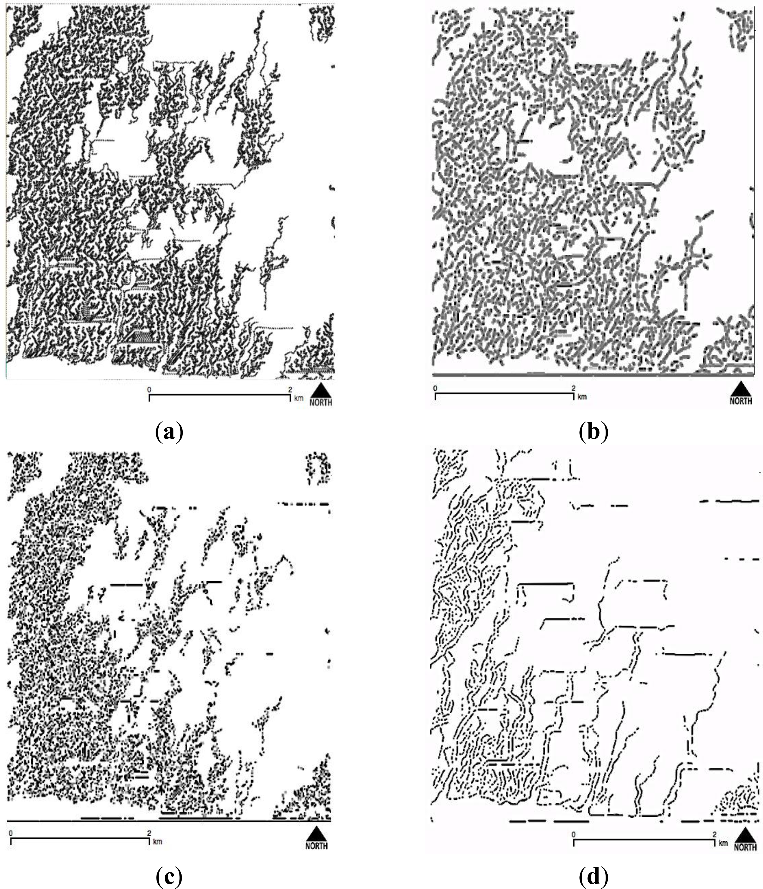
4.1. Performance Evaluation of the Edge Detection Methods on a Synthetic DEM
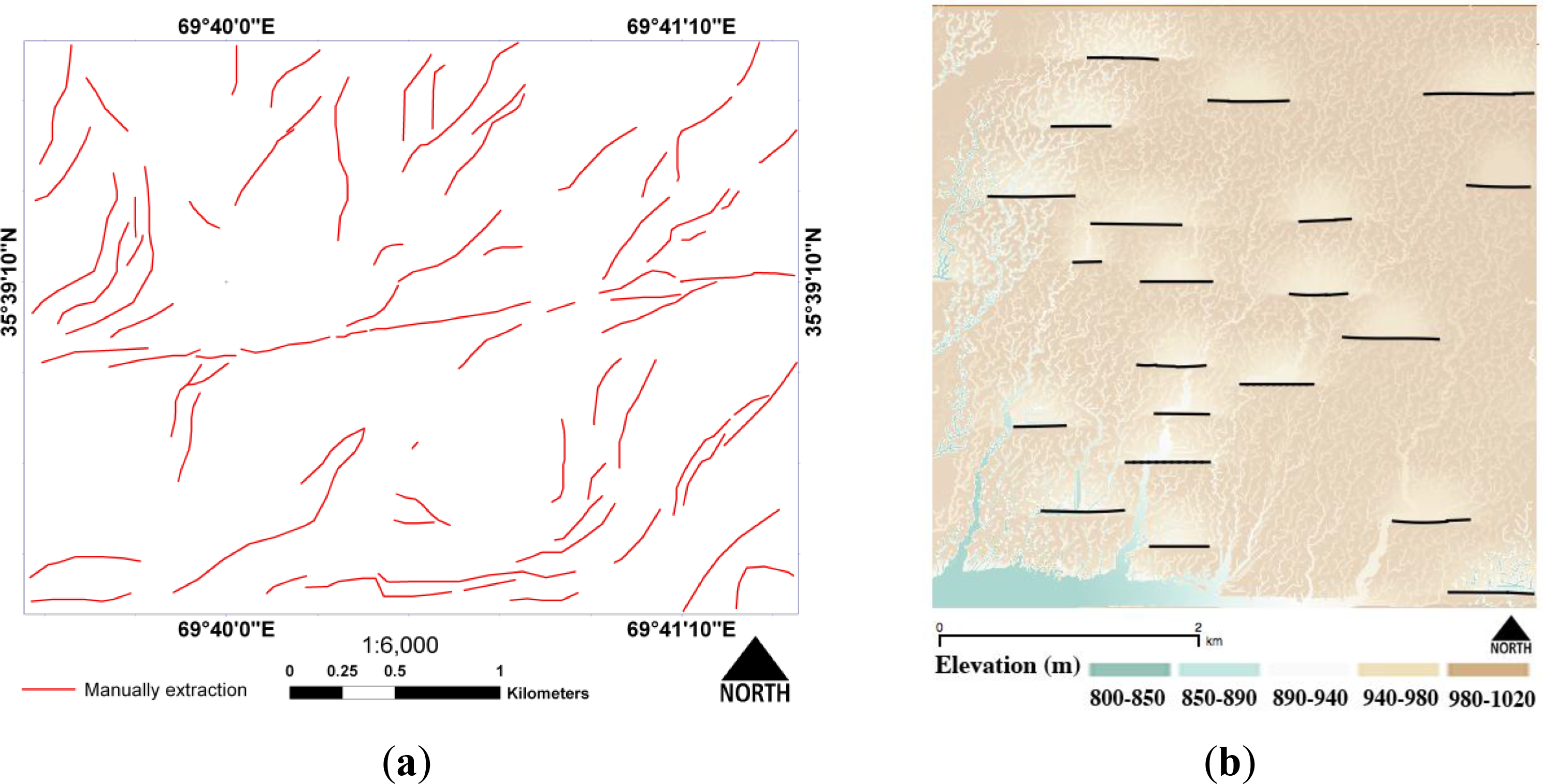
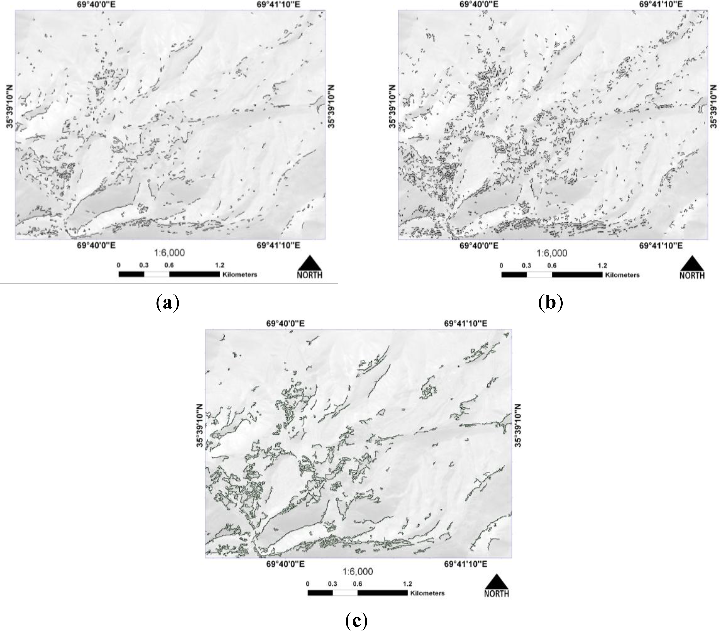
4.2. Performance Evaluation of the Edge Detection Methods on a Satellite Image
Accuracy Measurements
5. Conclusions
Acknowledgments
Author Contributions
Conflicts of Interest
References
- Şener, Ş.; Sener, E.; Karagüzel, R. Solid waste disposal site selection with GIS and AHP methodology: A case study in Senirkent–Uluborlu (Isparta) Basin, Turkey. Environ. Monit. Assess 2011, 173, 533–554. [Google Scholar]
- Mukherjee, S. Microzonation of seismic and landslide prone areas for alternate highway alignment in a part of western coast of India using remote sensing techniques. J. Indian Soc. Remote Sens 1999, 27, 81–90. [Google Scholar]
- Charnpratheep, K.; Zhou, Q.; Garner, B. Preliminary landfill site screening using fuzzy geographical information systems. Waste Manag. Res 1997, 15, 197–215. [Google Scholar]
- Rangzan, K.; Charchi, A.; Abshirini, E.; Dinger, J. Remote sensing and GIS approach for water-well site selection, southwest Iran. Environ. Eng. Geosci 2008, 14, 315–326. [Google Scholar]
- Riedel, M.; Collett, T.S.; Kumar, P.; Sathe, A.V.; Cook, A. Seismic imaging of a fractured gas hydrate system in the Krishna–Godavari Basin offshore India. Mar. Pet. Geol 2010, 27, 1476–1493. [Google Scholar]
- Bartolome, R.; Gràcia, E.; Stich, D.; Martínez-Loriente, S.; Klaeschen, D.; de Lis Mancilla, F.; Iacono, C.L.; Dañobeitia, J.J.; Zitellini, N. Evidence for active strike-slip faulting along the Eurasia-Africa convergence zone: Implications for seismic hazard in the southwest Iberian margin. Geology 2012, 40, 495–498. [Google Scholar]
- Safari, H.O.; Pirasteh, S.; Pradhan, B.; Gharibvand, L.K. Use of remote sensing data and GIS tools for seismic hazard assessment for shallow oilfields and its impact on the settlements at Masjed-I-soleiman area, Zagros Mountains, Iran. Remote Sens 2010, 2, 1364–1377. [Google Scholar]
- Gomez, H.; Kavzoglu, T. Assessment of shallow landslide susceptibility using artificial neural networks In jabonosa River Basin, Venezuela. Eng. Geol 2005, 78, 11–27. [Google Scholar]
- Neuhäuser, B.; Terhorst, B. Landslide susceptibility assessment using “weights-of-evidence” applied to a study area at the Jurassic Escarpment (SW-Germany). Geomorphology 2007, 86, 12–24. [Google Scholar]
- Geiß, C.; Taubenböck, H. Remote sensing contributing to assess earthquake risk: From a literature review towards a roadmap. Nat. Hazards 2013, 68, 7–48. [Google Scholar]
- Pradhan, B.; Lee, S. Landslide susceptibility assessment and factor effect analysis: Backpropagation artificial neural networks and their comparison with frequency ratio and bivariate logistic regression modelling. Environ. Model. Softw 2010, 25, 747–759. [Google Scholar]
- Comparison of Edge Detection and Hough Transform Techniques for the Extraction of Geologic Features. Available online: http://www.cartesia.org/geodoc/isprs2004/comm3/papers/376.pdf (accessed on 19 June 2014).
- Mabee, S.B.; Hardcastle, K.C.; Wise, D.U. A method of collecting and analyzing lineaments for regional-scale fractured-bedrock aquifer studies. Ground Water 1994, 32, 884–894. [Google Scholar]
- Chowdary, V.M.; Ramakrishnan, D.; Srivastava, Y.K.; Chandran, V.; Jeyaram, A. Integrated water resource development plan for sustainable management of mayurakshi watershed, India using remote sensing and GIS. Water Resour. Manag 2009, 23, 1581–1602. [Google Scholar]
- Mabee, S.B.; Curry, P.J.; Hardcastle, K.C. Correlation of lineaments to ground water inflows in a bedrock tunnel. Groundwater 2002, 40, 37–43. [Google Scholar]
- Krishnamurthy, J.; Venkatesa Kumar, N.; Jayaraman, V.; Manivel, M. An approach to demarcate ground water potential zones through remote sensing and a geographical information system. Int. J. Remote Sens 1996, 17, 1867–1884. [Google Scholar]
- Rowan, L.C.; Lathram, E.H. Chapter 17 Mineral Exploration. In Remote Sensing in Geology; Siegal, B.S., Gillespie, A.R., Eds.; John Wiley and sons: New York, NY, USA, 1980; pp. 553–605. [Google Scholar]
- Lee, M.; Morris, W.; Harris, J.; Leblanc, G. An automatic network-extraction algorithm applied to magnetic survey data for the identification and extraction of geologic lineaments. Lead. Edge 2012, 31, 26–31. [Google Scholar]
- Agterberg, F.P.; Bonham-Carter, G.F.; Wright, D.F. Statistical Pattern Integration for Mineral Exploration. In Computer Applications in Resource Estimation Prediction and Assessment for Metals and Petroleum; Pergamon Press: Oxford, UK, 1990; pp. 1–21. [Google Scholar]
- Sabins, F.F. Remote sensing for mineral exploration. Ore Geol. Rev 1999, 14, 157–183. [Google Scholar]
- Halbouty, M.T. Application of Landsat imagery to petroleum and mineral exploration. AAPG Bull 1976, 60, 745–793. [Google Scholar]
- Cooper, S.M. Potential field investigation of the Liberia Basin, west Africa. J. Am. Sci 2010, 6, 199–207. [Google Scholar]
- Bartholomew, I.D.; Peters, J.M.; Powell, C.M. Regional Structural Evolution of the North Sea: Oblique Slip and the Reactivation of Basement Lineaments. In Geological Society, London, Petroleum Geology Conference Series, 1993; Geological Society of London: London, UK, 1993; pp. 1109–1122. [Google Scholar]
- Salvini, F.; Storti, F. Cenozoic tectonic lineaments of the Terra Nova Bay Region, Ross Embayment, Antarctica. Glob. Planet. Chang 1999, 23, 129–144. [Google Scholar]
- Zevenbergen, L.W.; Thorne, C.R. Quantitative analysis of land surface topography. Earth Surf. Process. Landf 1987, 12, 47–56. [Google Scholar]
- Shahzad, F.; Gloaguen, R. Tecdem: A matlab based toolbox for tectonic geomorphology, part 1: Drainage network preprocessing and stream profile analysis. Comput. Geosci 2011, 37, 250–260. [Google Scholar]
- Karnieli, A.; Meisels, A.; Fisher, L.; Arkin, Y. Automatic extraction and evaluation of geological linear features from digital remote sensing data using a hough transform. Photogramm. Eng. Remote Sens 1996, 62, 525–531. [Google Scholar]
- Wladis, D. Automatic lineament detection using digital elevation models with second derivative filters. Photogramm. Eng. Remote Sens 1999, 65, 453–458. [Google Scholar]
- Wang, J.; Howarth, P.J. Use of the hough transform in automated lineament. Geosci. Remote Sens. IEEE Trans 1990, 28, 561–567. [Google Scholar]
- Moore, G.K.; Waltz, F.A. Objective procedures for lineament enhancement and extraction (digital convolution enhanced images). Photogramm. Eng. Remote Sens 1983, 49, 641–647. [Google Scholar]
- Gustafsson, P. Spot satellite data for exploration of fractured aquifers in a semi-arid area in southeastern Botswana. Appl. Hydrogeol 1994, 2, 9–18. [Google Scholar]
- Duda, R.O.; Hart, P.E. Pattern Classification and Scene Analysis; Wiley: New York, NY, USA, 1973. [Google Scholar]
- Prewitt, J.M.S. Object Enhancement and Extraction; Academic Press: New York, NY, USA, 1970. [Google Scholar]
- Morris, K. Using knowledge-base rules to map the three-dimensional nature of geological features. Photogramm. Eng. Remote Sens 1991, 57, 1209–1216. [Google Scholar]
- Suzen, M.L.; Toprak, V. Filtering of satellite images in geological lineament analyses: An application to a fault zone in central Turkey. Int. J. Remote Sens 1998, 19, 1101–1114. [Google Scholar]
- Marr, D.; Hildreth, E. Theory of edge detection. Proc. R. Soc. Lond. Ser. B Biol. Sci 1980, 207, 187–217. [Google Scholar]
- Tripathi, N.K.; Gokhale, K.; Siddiqui, M.U. Directional morphological image transforms for lineament extraction from remotely sensed images. Int. J. Remote Sens 2000, 21, 3281–3292. [Google Scholar]
- Fitton, N.C.; Cox, S.J.D. Optimising the application of the hough transform for automatic feature extraction from geoscientific images. Comput. Geosci 1998, 24, 933–951. [Google Scholar]
- Hough, P.V.C. Method and Means for Recognizing Complex Patterns, U.S. Patent 3069654. 18 December 1962.
- Duda, R.O.; Hart, P.E. Use of the hough transformation to detect lines and curves in pictures. Commun. ACM 1972, 15, 11–15. [Google Scholar]
- Koike, K.; Nagano, S.; Kawaba, K. Construction and analysis of interpreted fracture planes through combination of satellite-image derived lineaments and digital elevation model data. Comput. Geosci 1998, 24, 573–583. [Google Scholar]
- Argialas, D.P.; Harlow, C.A. Computational image interpretation models: An overview and a perspective. Photogramm. Eng. Remote Sens 1990, 56, 871–886. [Google Scholar]
- Karantzalos, K.; Argialas, D. Improving edge detection and watershed segmentation with anisotropic diffusion and morphological levellings. Int. J. Remote Sens 2006, 27, 5427–5434. [Google Scholar]
- Ziou, D.; Koukam, A. Knowledge-based assistant for the selection of edge detectors. Pattern Recognit 1998, 31, 587–596. [Google Scholar]
- Nguyen, T.B.; Ziou, D. Contextual and non-contextual performance evaluation of edge detectors. Pattern Recognit. Lett 2000, 21, 805–816. [Google Scholar]
- Heath, M.D.; Sarkar, S.; Sanocki, T.; Bowyer, K.W. A robust visual method for assessing the relative performance of edge-detection algorithms. IEEE Trans. Pattern Anal. Mach. Intell 1997, 19, 1338–1359. [Google Scholar]
- Cho, K.; Meer, P.; Cabrera, J. Performance assessment through bootstrap. Pattern Anal. Mach. Intell. IEEE Trans 1997, 19, 1185–1198. [Google Scholar]
- Lopez-Molina, C.; de Baets, B.; Bustince, H. Quantitative error measures for edge detection. Pattern Recognit 2013, 46, 1125–1139. [Google Scholar]
- Ji, Q.; Haralick, R.M. Efficient facet edge detection and quantitative performance evaluation. Pattern Recognit 2002, 35, 689–700. [Google Scholar]
- Román-Roldán, R.; Gómez-Lopera, J.F.; Atae-Allah, J; Martinez-Aroza, J.; Luque-Escamilla, P.L. A measure of quality for evaluating methods of segmentation and edge detection. Pattern Recognit 2001, 34, 969–980. [Google Scholar]
- Evaluation of Edge Detectors: Critics and Proposal. Available online: http://www.vision.auc.dk/~hic/perf-proc.html (accessed on 20 June 2014).
- Shin, M.C.; Goldgof, D.B.; Bowyer, K.W. Comparison of edge detector performance through use in an object recognition task. Comput. Vision Image Underst 2001, 84, 160–178. [Google Scholar]
- Heath, M.; Sarkar, S.; Sanocki, T.; Bowyer, K. Comparison of Edge Detectors: A Methodology and Initial Study, Computer Vision and Pattern Recognition, 1996. Proceedings of the 1996 IEEE Computer Society Conference on CVPR96, San Franciso, CA, USA, 18–20 June 1996; pp. 143–148.
- Pellegrino, F.A.; Vanzella, W.; Torre, V. Edge detection revisited. Syst. Man Cybern. Part B 2004, 34, 1500–1518. [Google Scholar]
- Yitzhaky, Y.; Peli, E. A method for objective edge detection evaluation and detector parameter selection. IEEE Trans. Pattern Anal. Mach. Intell 2003, 25, 1027–1033. [Google Scholar]
- Ambraseys, N.; Bilham, R. The Tectonic Setting of Bamiyan and the Seismicity in and Near Afghanistan for the Past 12 Centuries. In After the Destruction of Giant Buddha Statues in Bamiyan (Afghanistan) in 2001; Margottini, C., Ed.; Springer Berlin Heidelberg: Berlin, Germany, 2009; pp. 67–94. [Google Scholar]
- Map and Database of Probable and Possible Quaternary Faults in Afghanistan. Available online: http://pubs.usgs.gov/of/2007/1103/downloads/pdf/ofr07-1103plate.pdf (accessed on 20 June 2014).
- Wheeler, R.L.; Bufe, C.G.; Johnson, M.L.; Dart, R.L. Seismotectonic Map of Afghanistan, with Annotated Bibliography; US Department of the Interior, US Geological Survey: Reston, VA, USA, 2005. [Google Scholar]
- Ziou, D.; Tabbone, S. Edge detection techniques—An overview. Pattern Recognit. Image Anal 1998, 8, 537–559. [Google Scholar]
- Canny, J. A computational approach to edge detection. IEEE Trans. Pattern Anal. Mach. Intell 1986, PAMI-8, 679–698. [Google Scholar]
- Deriche, R. Using cannys criteria to derive a recursively implemented optimal edge detector. Int. J. Comput. Vision 1987, 1, 167–187. [Google Scholar]
- Ziou, D. Line detection using an optimal IIR filter. Pattern Recognition 1991, 24, 465–478. [Google Scholar]
- Maini, R.; Aggarwal, H. Study and comparison of various image edge detection techniques. Int. J. Image Process. (IJIP) 2009, 3, 1–11. [Google Scholar]
- Edge Detection Analysis. Available online: http://disp.ee.ntu.edu.tw/meeting/%E8%87%AA%E6%81%86/edge%20detection/edge_detection.pdf (accessed on 19 June 2014).
- Pratt, W.K. Digital Image Processing. In Image Enhancement; Wiley-Interscience: New York, NY, USA, 2007; pp. 247–307. [Google Scholar]
- Chai, H.Y.; Wee, L.K.; Supriyanto, E. Edge Detection in Ultrasound Images Using Speckle Reducing Anisotropic Diffusion in Canny Edge Detector Framework. Proceedings of the 15th WSEAS International Conference on SYSTEMS, Corfu Island, Greece, 14–16 July 2011; pp. 226–231.
- Gonzalez, R.C.; Woods, R.E.; Eddins, S.L. Digital Image Processing Using Matlab; Gatesmark Publishing: Knoxville, TN, USA, 2009. [Google Scholar]
- Han, C.; Kerwin, W.S.; Hatsukami, T.S.; Hwang, J.-N.; Yuan, C. Detecting objects in image sequences using rule-based control in an active contour model. IEEE Trans. Biomed. Eng 2003, 50, 705–710. [Google Scholar]
- Sonka, M.; Hlavac, V.; Boyle, R. Image Processing, Analysis, and Machine Vision; Springer: Berlin, Germany, 1999. [Google Scholar]
- Tensor Voting: Theory and Applications. Available online: http://www.sci.utah.edu/~gerig/CS7960-S2010/handouts/Medioni_tensor_voting.pdf (accessed on 19 June 2014).
- Mordohai, P.; Medioni, G. Tensor voting: A perceptual organization approach to computer vision and machine learning. Synth. Lect. Image Video Multimed. Process 2006, 2, 1–136. [Google Scholar]
- Loss, L.; Bebis, G.; Nicolescu, M.; Skurikhin, A. An iterative multi-scale tensor voting scheme for perceptual grouping of natural shapes in cluttered backgrounds. Comput. Vision Image Underst 2009, 113, 126–149. [Google Scholar]
- Abdou, I.E.; Pratt, W. Quantitative design and evaluation of enhancement/thresholding edge detectors. Proc. IEEE 1979, 67, 753–763. [Google Scholar]
- Kanungo, T.; Jaisimha, M.Y.; Palmer, J.; Haralick, R.M. A methodology for quantitative performance evaluation of detection algorithms. IEEE Trans. Image Proc 1995, 4, 1667–1674. [Google Scholar]
- Mokhtarian, F.; Mohanna, F. Performance evaluation of corner detectors using consistency and accuracy measures. Comput. Vision Image Underst 2006, 102, 81–94. [Google Scholar]
- Viola, P.; Jones, M. Rapid Object Detection Using a Boosted Cascade of Simple Features, CVPR 2001. Proceedings of the 2001 IEEE Computer Society Conference on Computer 2011 Vision and Pattern Recognition, Kauai, HI, USA, 8–14 December 2001; pp. I-511–I-518.
- Lu, D.-S.; Chen, C.-C. Edge detection improvement by ant colony optimization. Pattern Recognit. Lett 2008, 29, 416–425. [Google Scholar]
- Manish, T.I.; Murugan, D.; Kumar, G. Hybrid edge detection using canny and ant colony optimization. Commun. Inf. Sci. Manag. Eng. 2013, 3, 402–405. [Google Scholar]
- Koike, K.; Nagano, S.; Ohmi, M. Lineament analysis of satellite images using a Segment Tracing Algorithm (STA). Comput. Geosci 1995, 21, 1091–1104. [Google Scholar]
- Novak, I.D.; Soulakellis, N. Identifying geomorphic features using Landsat-5/TM data processing techniques on Lesvos, Greece. Geomorphology 2000, 34, 101–109. [Google Scholar]
- Mallast, U.; Gloaguen, R.; Geyer, S.; Rodiger, T.; Siebert, C. Derivation of groundwater flow-paths based on semi-automatic extraction of lineaments from remote sensing data. Hydrol. Earth Syst. Sci 2011, 15, 2665–2678. [Google Scholar] [Green Version]
- Kirby, E.; Whipple, K. Quantifying differential rock-uplift rates via stream profile analysis. Geology 2001, 29, 415–418. [Google Scholar]
- Gloaguen, R.; Kabner, A.; Wobbe, F.; Shahzad, F.; Mahmood, A. Remote Sensing Analysis of Crustal Deformation Using River Networks. In. Proceedings of the IEEE International Conference on Geoscience and Remote Sensing Symposium, IGARSS 2008, Boston, MA, USA, 7–11 July 2008; pp. IV-1–IV-4.
- Gloaguen, R.; Marpu, P.R.; Niemeyer, I.; Alonso, C.; Castellanos, M.T.; Redondo, J.M. Automatic extraction of faults and fractal analysis from remote sensing data. Nonlinear Process. Geophys 2007, 14, 131–138. [Google Scholar]
- Kurz, T.; Gloaguen, R.; Ebinger, C.; Casey, M.; Abebe, B. Deformation distribution and type in the Main Ethiopian Rift (MER): A remote sensing study. J. Afr. Earth Sci 2007, 48, 100–114. [Google Scholar]
- Shahzad, F.; Gloaguen, R. Tecdem: A matlab based toolbox for tectonic geomorphology, part 2: Surface dynamics and basin analysis. Comput. Geosci 2011, 37, 261–271. [Google Scholar]
- Tectonic Lineament Analysis using Remote Sensing Datasets Tollbox (TecLines). Available online: http://www.teclines.net (accessed on 19 June 2014).


| Feature | λ1λ2 | e1e2 | Tensor | Saliency | Normal | Tangent | Normal | Tensor |
|---|---|---|---|---|---|---|---|---|
| Point | 1 | 1 | Any orthonormal basis | Ball | λ1 all2 > 1 | None | Any orthonormal basis | None |
| Curve | 1 | 0 | n t | Stick | λ1 − λ2 > λ2 | e1 | e2 | e1 |
| Method | TP | FP | FN | Overall Accuracy (%) | |
|---|---|---|---|---|---|
| Without Butterworth band-pass filtering | Canny | 360 | 26,370 | 820 | 15.9 |
| Canny + TVF | 480 | 17,380 | 700 | 21.6 | |
| With Butterworth band-pass filtering | Canny | 920 | 12,240 | 260 | 42.4 |
| Canny + TVF | 1098 | 8339 | 82 | 52.3 | |
| Method | TP | FP | FN | Overall Accuracy (%) |
|---|---|---|---|---|
| Sobel | 3726 | 8657 | 2464 | 42.7 |
| Sobel + TVF | 4333 | 1075 | 1857 | 64.8 |
| LOG | 3838 | 9721 | 2352 | 43.1 |
| LOG + TVF | 4271 | 1684 | 1919 | 60.62 |
| Canny | 4147 | 6293 | 2043 | 46.5 |
| Canny + TVF | 4891 | 795 | 1299 | 74.5 |
© 2014 by the authors; licensee MDPI, Basel, Switzerland This article is an open access article distributed under the terms and conditions of the Creative Commons Attribution license (http://creativecommons.org/licenses/by/3.0/).
Share and Cite
Rahnama, M.; Gloaguen, R. TecLines: A MATLAB-Based Toolbox for Tectonic Lineament Analysis from Satellite Images and DEMs, Part 1: Line Segment Detection and Extraction. Remote Sens. 2014, 6, 5938-5958. https://doi.org/10.3390/rs6075938
Rahnama M, Gloaguen R. TecLines: A MATLAB-Based Toolbox for Tectonic Lineament Analysis from Satellite Images and DEMs, Part 1: Line Segment Detection and Extraction. Remote Sensing. 2014; 6(7):5938-5958. https://doi.org/10.3390/rs6075938
Chicago/Turabian StyleRahnama, Mehdi, and Richard Gloaguen. 2014. "TecLines: A MATLAB-Based Toolbox for Tectonic Lineament Analysis from Satellite Images and DEMs, Part 1: Line Segment Detection and Extraction" Remote Sensing 6, no. 7: 5938-5958. https://doi.org/10.3390/rs6075938