Article

Evaluation of Daytime Evaporative Fraction from MODIS TOA Radiances Using FLUXNET Observations

Max Planck Institute for Meteorology, 20146 Hamburg, Germany
*
Author to whom correspondence should be addressed.
Remote Sens. 2014, 6(7), 5959-5975; https://doi.org/10.3390/rs6075959
Submission received: 9 February 2014 / Revised: 6 June 2014 / Accepted: 6 June 2014 / Published: 25 June 2014

Abstract

:
In recent decades, the land surface temperature/vegetation index (LST/NDVI) feature space has been widely used to estimate actual evapotranspiration (ETa) or evaporative fraction (EF, defined as the ratio of latent heat flux to surface available energy). Traditionally, it is essential to pre-process satellite top of atmosphere (TOA) radiances to obtain LST before estimating EF. However, pre-processing TOA radiances is a cumbersome task including corrections for atmospheric, adjacency and directional effects. Based on the contextual relationship between LST and NDVI, some studies proposed the direct use of TOA radiances instead of satellite retrieved LST products to estimate EF, and found that use of TOA radiances is applicable in some regional studies. The purpose of the present study is to test the robustness of the TOA radiances based EF estimation scheme over different climatic and surface conditions. Flux measurements from 16 FLUXNET (a global network of eddy covariance towers) sites were used to validate the Moderate Resolution Imaging Spectro radiometer (MODIS) TOA radiances estimated daytime EF. It is found that the EF estimates perform well across a wide variety of climate and biome types—Grasslands, crops, cropland/natural vegetation mosaic, closed shrublands, mixed forest, deciduous broadleaf forest, and savannas. The overall mean bias error (BIAS), mean absolute difference (MAD), root mean square difference (RMSD) and correlation coefficient (R) values for all the sites are 0.018, 0.147, 0.178 and 0.590, respectively, which are comparable with published results in the literature. We conclude that the direct use of measured TOA radiances instead of LST to estimate daytime EF can avoid complex atmospheric corrections associated with the satellite derived products, and would facilitate the relevant applications where minimum pre-processing is important.

1. Introduction

Mapping of the land surface heat fluxes and modeling the mass and energy interactions between land and atmosphere are significant for better understanding the mechanism of climate change, and plays a crucial role in hydrological, agricultural and meteorological studies [1,2]. The complicated physical mechanisms such as turbulent transport, the feedback in the soil-plant-atmosphere continuum and the heterogeneity of land surface all combine to make estimation of energy balance components a challenge [3,4]. Nevertheless, much work has been done in surface turbulent fluxes and partitioning among energy balance components [57]. As one fundamental parameter of surface heat fluxes, the evaporative fraction (EF, defined as the ratio of latent heat flux to available energy) represents the surface control on latent heat and sensible heat fluxes portioning [8,9]. Considering the spatial and temporal variability of the EF characteristic, satellite remote sensing is recognized as a promising technique to provide reasonable EF estimates over large areas and continents [10]. The approaches proposed in the literature use either empirical or physically based schemes [1113].
One popular method among them is using the relationship between land surface temperature (LST) and normalized difference vegetation index (NDVI) [14]. If the satellite derived LST and NDVI over heterogeneous areas are plotted, the shape of the pixel envelope resembles a physically meaningful triangular or trapezoidal feature space (Figure 1). The physical properties encapsulated in the LST/NDVI space are simple: The LST has low sensitivity over vegetated areas, but increased sensitivity over bare soil regions. The wet edge presents high EF because it has high thermal inertia and strong evaporative cooling. In contrast, the lowest EF occurs at dry edge due to its weakest evaporative cooling [15,16]. The LST/NDVI method is unique in interpreting the spatial variations of LST and NDVI to infer EF without largely depending on information from ground-based observations. Due to its simplicity and relatively high accuracy, this type of approach has already been widely accepted and used [1719]. The main limitation of the triangle method is that a large number of pixels over a flat area with a wide range of soil wetness and fractional vegetation cover are required to make sure that the dry and wet limits exist in the triangular space, and at the same time relatively uniform atmospheric forcing [2022]. For a detailed description and discussion of the LST/NDVI triangle feature space method, the reader is referred to the reviews given by Carlson et al. [23] and Petropoulos et al. [24].
The notable advantage of this method is that it needs only satellite data to retrieve EF with minimum requirements of model inputs and ancillary data [25]. However, when satellite data are used to represent traditionally ground-based measurement, such as LST, correcting satellite data based on radiative transfer theory are necessary. Because the information received by the satellite sensors is TOA (Top of Atmosphere) radiances that are affected by viewing angles and atmospheric variables [26]. This actually poses great challenges for the remote sensing community to develop different correction procedures to eliminate the atmospheric attenuation effects [27]. Although much effort has been devoted to establish sophisticated and streamlined data correction procedures, these procedures are troublesome and need independent observation data to satisfy the mathematical and physical constraints. These limitations practically increase the operational difficulty. Under this background, several studies focus on the EF estimation from the TOA radiances rather than satellite products, and found that use of TOA radiances is adequate to estimate EF [2830]. The feasibility of estimating EF using TOA radiances stems from the contextual relationship between LST and NDVI. For applications that depend on contextual information from remote sensing, absolute radiometric calibration to remote sensing data is thought to be unnecessary [31,32]. A recent study by Peng et al. [33] investigated the general possibility of estimating Normalized Difference Temperature Index (NDTI, a key parameter for EF estimation) from TOA radiances through a physical understanding of Planck radiation law and radiative transfer equation, and performed a detailed sensitivity analysis of NDTI on surface and atmosphere variability. They concluded that the TOA radiances based estimates have similar level of accuracy as obtained using atmospherically corrected data products. However, as indicated by Peng et al. [28,33], more validation work of TOA radiances retrieved EF against ground-based measurements over different climatic and surface conditions still needs to be carried out.
The main objective of this study is to evaluate the applicability and robustness of the TOA radiances based daytime EF estimation scheme through comparison with measurements from 16 FLUXNET (a global network of eddy covariance towers) sites, which have already been widely used for validation of estimates from remote sensing [34,35]. These sites represent a wide range of climates and biome types—grasslands, crops, cropland/natural vegetation mosaic, closed shrublands, mixed forest, deciduous broadleaf forest, and savannas.

2. Materials and Methodology

2.1. Remote Sensing Data

Moderate Resolution Imaging Spectro radiometer (MODIS) is the primary satellite sensor in the NASA Earth Observing System (EOS) for land, ocean and atmosphere research [36]. Specifically, the Terra-MODIS Collection 5 data products used in this study mainly include MOD021KM, MOD03, MOD09GA and MOD35_L2. The MOD021KM (band 31) and MOD03 datasets are used to provide geolocated and calibrated thermal band TOA radiance. In addition, the MOD09GA product contains surface reflectance that is used to calculate NDVI in this study. It should be noted that the MODIS data used in this work were transformed from Hierarchical Data Format-Earth Observation System (HDF-EOS) swath format to a Universal Transverse Mercator (UTM) projected GeoTIFF image and resampleed for 1 km pixel size. A prerequisite for the applicability of the LST/NDVI method are homogeneous atmospheric conditions and flat topography. A square domain was therefore defined around each flux tower site and was used as the study area for the subsequent processing. The size of each domain is about 60,000 km2, representing a wide range of fractional vegetation cover and soil wetness. On the basis of MOD35_L2 cloud mask product, the clear sky condition was identified when larger than 85% of the study domain being clear. The number of clear sky days (clear sky at MODIS overpass time) for each flux site is shown in Table 1.

2.2. FLUXNET Observations
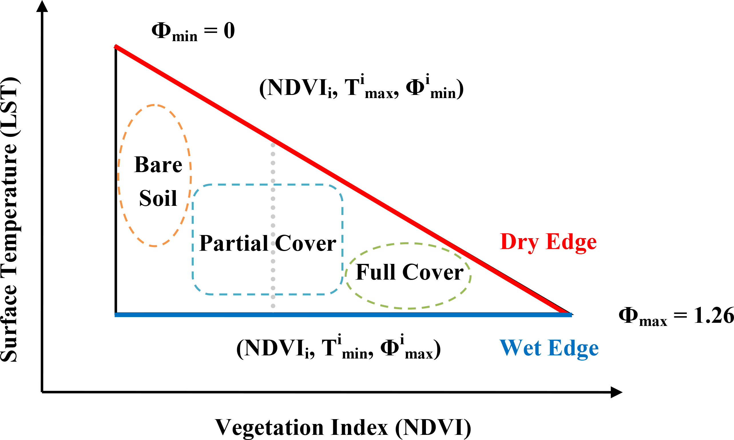
The publicly available FLUXNET observations were used to validate TOA radiances estimated EF. Through a suit of instruments, the flux towers can measure half-hourly averaged fluxes (net radiation, soil heat flux, latent heat flux and sensible heat flux) and meteorological data (e.g., air temperature, precipitation). The relevant FLUXNET methodologies and summaries could be found in the research of Aubinet et al. [37] and Baldocchi et al. [38]. In this study, 16 FLUXNET sites were selected mainly according to the following criteria: (1) the land cover for the 1 km2 area centered on the flux tower is homogeneous; (2) the land cover for a 10,000 km2 area encompassing the flux tower is heterogeneous with a range of fractional vegetation cover, and the terrain of the area is also flat. More information about these sites is given in Table 1 [3952].
These sites are located across Europe, North America and Africa and cover a broad range of land cover types (Table 1). According to the IGBP (International Geosphere-Biosphere Program) classification scheme, the sites are classified into seven main groups: grasslands, crops, cropland/natural vegetation mosaic, closed shrublands, mixed forest, deciduous broadleaf forest, and savannas. Further details about these sites are provided by the corresponding publications and references therein.
The eddy covariance technique is known to have problems with energy balance closure [5355]. Therefore, the eddy covariance measured heat fluxes need to be corrected for energy balance closure .One commonly used approach is the Bowen ratio method, which repartitions the mismatch in the energy budget closure in accordance to the Bowen ratio observed. Thus, the basic assumption is that the error in the budget closure can be distributed proportional to the ratio of the turbulent fluxes [54]. Since this method is relatively simple and accurate, and has been successfully used by many applications [5658], we also applied the method in the present study to correct the eddy covariance measured latent and sensible heat fluxes.

2.3. Methodology

According to the definition of EF, the instantaneous EF (dimensionless) calculated from instantaneous flux tower measurements can be written as:
EF ( t ) = LE ( t ) R n ( t ) G ( t ) = LE ( t ) LE ( t ) + H ( t )
where Rn is the surface net radiation (W·m−2), G is the ground heat flux (W·m−2), LE is latent heat flux (W·m−2) and H the sensible heat flux (W·m−2) at time t. Meanwhile, the daytime EF is determined using the following equation [10]:
EF daytime = t 1 t 2 LE ( t ) dt t 1 t 2 [ H ( t ) + LE ( t ) ] dt
where the time difference t2t1 refers to the time from 8:00 LT to 17:00 LT in the present study. The daytime rather than daily was selected as study period, because the eddy covariance technique is more reliable during daytime [59]. The daytime EF can also be estimated by averaging instantaneous EF from different time periods. The two approaches would have similar results if EF is stable during daytime [10,60]. In practice, the latter approach is more sensitive to the errors in LE and H measurements when they have low absolute values during early morning and late afternoon.
On the basis of the LST/NDVI feature space obtained from plotting remotely sensed LST against NDVI, the parameterization of instantaneous EF using TOA radiances is given as follows:
EF = ϕ Δ Δ + γ
where Δ is the slope of saturated vapor pressure at the air temperature (kPa·K−1) and γ is the psychrometric constant (kPa·K−1) [61]. ϕ combines the effects of Budyko–Thornthwaite–Mather wetness parameter and Priestley Taylor coefficient, which accounts for aerodynamic and canopy resistances [62]. In this study, ϕ is calculated using TOA radiances rather than LST products:
ϕ = ϕ max L max L s L max L min
where ϕmax is the maximum ϕ without surface water stress and often set to 1.26 [63]. Ls is the observed TOA radiance for a given pixel whose NDVI value is NDVIi, Lmax and Lmin are the corresponding highest and smallest TOA radiance which have the same NDVIi value. In order to obtain the value of ϕ for each pixel, a three-step linear interpolation scheme based on the LST/NDVI triangle (Figure 1) is used in the following manner [14]: (1) determine the dry and wet edges in the triangular space; (2) the global minimum and maximum ϕ are respectively set to ϕmin = 0 for the driest bare soil pixel and ϕmax = 1.26 for the densely vegetated pixel with largest NDVI and lowest TOA radiance, then ϕimin is linearly interpolated for each NDVI interval (NDVIi) between ϕmin and ϕmax, and ϕimax for each NDVIi is obtained from the lowest TOA radiance pixel with that NDVI interval (ϕimax is generally set to ϕimax = ϕmax =1.26); (3) ϕi value within each NDVI interval is interpolated between the lowest TOA radiance pixel and highest TOA radiance pixel. Consequently, the ϕ value for each pixel can be calculated using Equation (4).

2.4. Algorithm Evaluation

A number of quantitative indices, including mean bias error (BIAS), mean absolute difference (MAD), root mean square difference (RMSD), relative error (RE) and correlation coefficient (R) are selected in this study to evaluate the model performance [64]. Furthermore, the results were also compared with published studies.

3. Results and Discussion

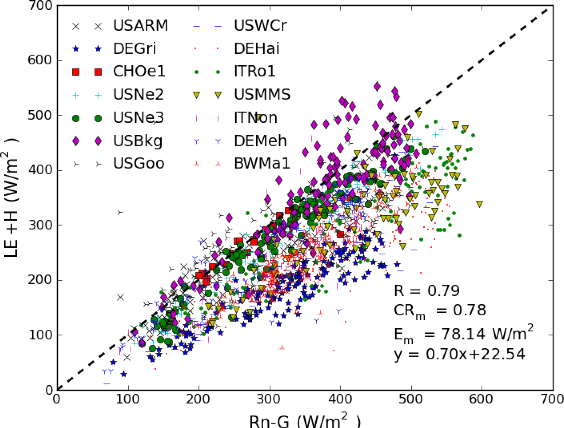
3.1. Energy Imbalance of Flux Tower Measurements

The energy closure of the flux tower measurements was investigated for the selected clear sky case days. Figure 2 shows the comparisons of observed daytime average available energy Rn − G against measured turbulent fluxes LE + H after correction for energy balance closure for all the FLUXNET sites except CASF2 and CASF3, because these two sites both have no G measurements. The closure ratio CR = (LE + H)/(Rn − G) varies from 0.57 to 0.98 with residual energy E = Rn − LE − H − G ranging from −136.53 to − 8.83 W/m2 at all the sites. Overall, the S (slope) and R from the linear least squares regression for observed LE + H and Rn − G are 0.70 and 0.79, respectively. It can also be seen that the measured LE + H fluxes are generally less than Rn − G for all these sites with the averaged closure ratio CRm of 0.78 and mean residual energy Em of 78.14 W/m2. Similar results were reported by Wilson et al. [55] and Foken [65]. However, the causes of the lack of energy balance closure are still under discussion and might be related to systematic bias in instrumentation, neglected energy sinks, landscape heterogeneity and mismatch in source areas.

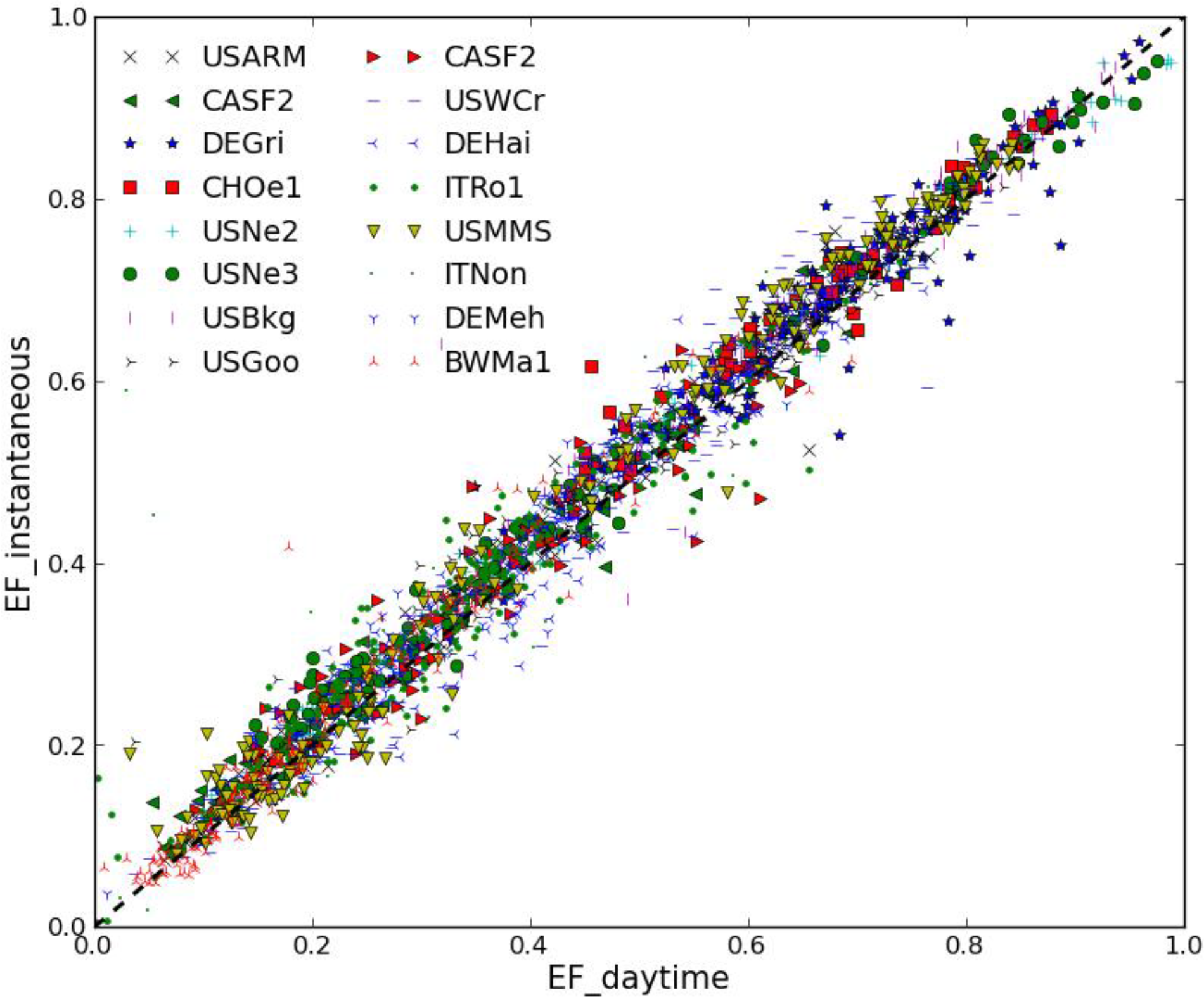
3.2. Can Near Noon Instantaneous EF Represent Daytime EF?

The EF has been found to be stable during daylight hours in many studies [11,66,67], making it possible to extrapolate instantaneous EF values to daytime scale. In this study, the instantaneous EF at MODIS overpass time was used to represent daytime EF value. To examine the feasibility of this assumption, the FLUXNET measurements were used to respectively estimate instantaneous and daytime EF using Equations (1) and (2). Figure 3 shows the comparison between the instantaneous EF at the time of MODIS overpass and the daytime EF for all the FLUXNET sites in our study. Table 2 presents the BIAS, MAD, RMSD, RE and R values for every FLUXNET site. It can be seen that these statistical indices values range from −0.035 to −0.011 for BIAS, from 0.023 to 0.050 for MAD, from 0.031 to 0.084 for RMSD, from −7.19% to −2.82% for RE and from 0.931 to 0.996 for R. On the whole, a good agreement and negligible bias between the instantaneous and daytime EF is obtained with BIAS = −0.020, MAD = 0.031, RMSD = 0.042 and RE (Relative Error) = −4.47% for all the sites. Besides, it can be observed that R = 0.977 (Table 2). These statistics results indicate the reliability of using EF constant assumption to estimate daytime EF without incurring substantial errors.

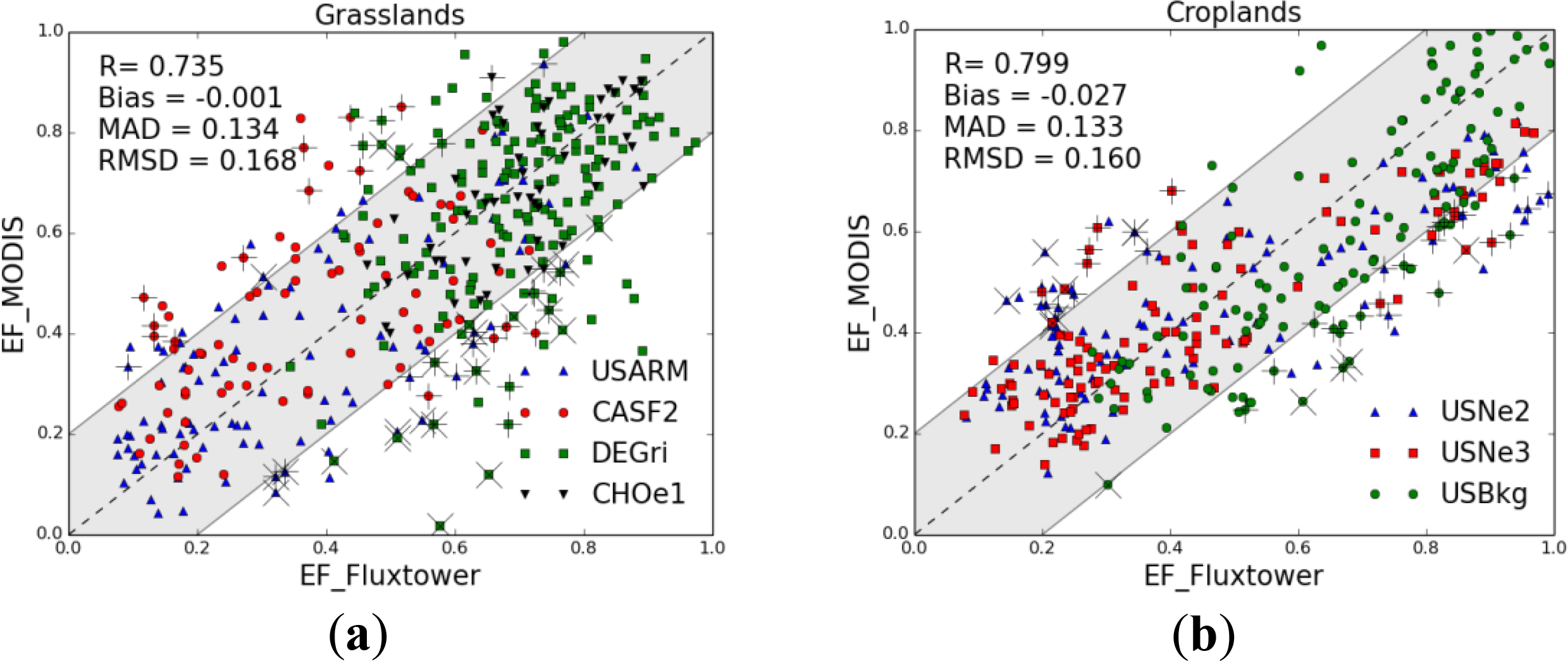
3.3. Evaluation of Daytime EF from MODIS TOA Radiances

The MODIS TOA radiances estimated daytime EF is evaluated with FLUXNET measured daytime EF. The comparison results are illustrated by Figure 4. In general, the derived EF agrees well with tower-measured EF with data points distributed around the dashed 1:1 line without a significant discrepancy. The grasslands, croplands, cropland/natural vegetation mosaic and mixed forest show good accuracy, whereas the savannas have slightly poorer performance. It may be attributed to its lack of full range of vegetation cover and surface temperature. The implicit assumption of the triangle method is that ETa primarily depends on soil moisture and vegetation cover. This assumption requires a heterogeneous area with a full range of possible soil moisture and vegetation fraction values, and at the same time relatively uniform atmospheric forcing [20]. The poor performance of savannas further demonstrate the limitation of triangle method.
Table 3 gives a comprehensive summary of the statistical metrics for each FLUXNET site. It can be observed that the BIAS values range from −0.08 to 0.12. The RMSD values vary from 0.103 to 0.224, and the R values appear to be low to high ranging from −0.280 to 0.846. The overall BIAS, MAD, RMSD and R values for all the sites are 0.018, 0.147, 0.178 and 0.590, respectively. This suggests the feasibility of estimating EF with MODIS TOA radiances alone. If we excluded the results of savannas, the BIAS, MAD and RMSD are further reduced to 0.006, 0.138, and 0.168 with a better R of 0.648. The LST/NDVI feature space has already extensively been used to estimate EF. The performance of this method has also been reported in the literature and it has been shown that EF estimates based on TOA radiances result in comparable results than using products of geophysical surface variables [28,68]. Table 4 summarizes the statistics of the differences between satellite products derived EF and observed EF from previous published studies. It can be seen that the statistical results found in this study are comparable to those reported previously. It further suggests that using TOA radiances can provide reasonable estimation accuracy for EF, while requiring less input data and preprocessing like in classical LST/NDVI feature space approaches.
In terms of error assessment, most discrepancies between estimated and measured EF are less than 0.2, presented in Figure 4. On the basis of semi-empirical error analysis, Jiang et al. [69] found that the upper bounds of absolute error and relative error in LST/NDVI estimated EF are less than 0.25% and 33.3%, respectively. As precipitation could introduce a large error of EF estimation through enhancing soil moisture and leaf interception, we used plus symbols to indicate the days contaminated by precipitation which occurred before satellite overpass. Besides, Wang and Dickinson [7] found that the LST/NDVI method is most suitable for a growing season in middle latitude areas. Because the key assumption of triangle method is that the ETa is negatively correlated with surface temperature.
However, the ETa in high latitudes and cold areas is generally positively correlated with temperature [70,71]. In other words, the range of vegetation index should be large enough, and the soil moisture rather than air temperature or available energy is the key control of EF. It means the sample days that are not during growing season will have more uncertainties, which is in accordance with our results. In Figure 4, the points with x markers are the samples days outside the growing season. Furthermore, the use of TOA radiances itself can introduce slight errors, as Peng et al. [33] found that NDTI can be estimated from TOA radiances with an accuracy of 90%. Other sources of uncertainty of our results could be related to the scale discrepancy between the FLUXNET footprint measurements and satellite pixel estimates [35,72,73], the relative error between instantaneous EF and daily EF, as well as the linear parameterization of ϕ (without inclusion of wind speed and surface humidity) within the LST/NDVI feature space. Considering the simplicity and acceptable accuracy level of the LST/NDVI method, we conclude that the use of TOA radiances appears to be adequate for the estimation of EF, and would facilitate direct use of remote sensing data for the situations (e.g., multi-sensor studies, data assimilation) where minimum pre-processing is important.

4. Conclusions

The evaporative fraction (EF, defined as the ratio of latent heat flux to surface available energy) has been estimated from top of atmosphere (TOA) radiances instead of satellite retrieved land surface temperature (LST) products in some regional studies. In order to comprehensively examine the robustness of the TOA radiances based EF estimation scheme over different climate and surface conditions, flux measurements from 16 FLUXNET (a global network of eddy covariance towers) sites were used to validate the daytime EF estimated from Moderate Resolution Imaging Spectro radiometer (MODIS) TOA radiances. It was found that the EF estimated from TOA radiances perform well across a wide variety of climate conditions and biome types. The accuracy level is also comparable with published results in the literature. Besides, using FLUXNET measurements, the instantaneous EF is also found to be applicable for representing daytime EF, without incurring substantial errors. Overall, the present study, together with the work by Peng et al. [28,33] demonstrated that the direct use of measured TOA radiances instead of satellite retrieved LST products to estimate EF is feasible and applicable. The notable advantage of this approach is that no atmospheric corrections are required. This would facilitate data assimilation and multi-sensor studies due to minimal pre-processing requirements. The problem of using polar-orbiting satellites data such as MODIS is the temporal gaps due to cloud cover. One possible solution is utilizing the geostationary satellites data with high temporal resolution. Future work will examine the full capacities of the TOA radiances approach for geostationary satellites data.

Acknowledgments

The authors would like to thank the FLUXNET community for making the data public available as well as the principal investigators and collaborators of these sites. The MODIS datasets used in this study were obtained from the Level 1 and Atmosphere Archive and Distribution System (LAADS). We thank Friedrich Richter for his assistance with downloading MODIS data. The work was supported by the Cluster of Excellence CliSAP (EXC177), University of Hamburg, funded through the German Science Foundation (DFG), and the project of Yunnan Social Development (2012CA021). The authors would also like to thank the editors and anonymous reviewers for their comments and suggestions that highly improved the manuscript.

Author Contributions

Both authors made significant contributions to the manuscript. Jian Peng carried out the research, analyzed the results, and wrote the manuscript. Alexander Loew supervised the research, provided guidance on analysis of the results, and revised the manuscript.

Conflicts of Interest

The authors declare no conflict of interest.

References

  1. Jung, M.; Reichstein, M.; Ciais, P.; Seneviratne, S.I.; Sheffield, J.; Goulden, M.L.; Bonan, G.; Cescatti, A.; Chen, J.; de Jeu, R. Recent decline in the global land evapotranspiration trend due to limited moisture supply. Nature 2010, 467, 951–954. [Google Scholar]
  2. Sellers, P.; Dickinson, R.; Randall, D.; Betts, A.; Hall, F.; Berry, J.; Collatz, G.; Denning, A.; Mooney, H.; Nobre, C. Modeling the exchanges of energy, water, and carbon between continents and the atmosphere. Science 1997, 275, 502–509. [Google Scholar]
  3. Lettau, H. Evapotranspiration climatonomy. Mon. Weather Rev 1969, 97, 691–699. [Google Scholar]
  4. Rodriguez-Iturbe, I. Ecohydrology: A hydrologic perspective of climate-soil-vegetation dynamics. Water Resour. Res 2000, 36, 3–9. [Google Scholar]
  5. Farahani, H.J.; Howell, T.A.; Shuttleworth, W.J.; Bausch, W.C. Evapotranspiration: Progress in measurement and modeling in agriculture. Trans. ASABE 2007, 50, 1627–1638. [Google Scholar]
  6. Kalma, J.; McVicar, T.; McCabe, M. Estimating land surface evaporation: A review of methods using remotely sensed surface temperature data. Surv. Geophys 2008, 29, 421–469. [Google Scholar]
  7. Wang, K.; Dickinson, R.E. A review of global terrestrial evapotranspiration: Observation, modeling, climatology, and climatic variability. Rev. Geophys 2012, 50, RG2005. [Google Scholar]
  8. Bateni, S.M.; Entekhabi, D.; Castelli, F. Mapping evaporation and estimation of surface control of evaporation using remotely sensed land surface temperature from a constellation of satellites. Water Resour. Res 2013, 49, 950–968. [Google Scholar]
  9. Caparrini, F.; Castelli, F.; Entekhabi, D. Mapping of land-atmosphere heat fluxes and surface parameters with remote sensing data. Bound.-Layer Meteorol 2003, 107, 605–633. [Google Scholar]
  10. Wang, K.; Li, Z.; Cribb, M. Estimation of evaporative fraction from a combination of day and night land surface temperatures and NDVI: A new method to determine the priestley–taylor parameter. Remote Sens. Environ 2006, 102, 293–305. [Google Scholar]
  11. Caparrini, F.; Castelli, F.; Entekhabi, D. Estimation of surface turbulent fluxes through assimilation of radiometric surface temperature sequences. J. Hydrometeorol 2004, 5, 145–159. [Google Scholar]
  12. Gómez, M.; Olioso, A.; Sobrino, J.A.; Jacob, F. Retrieval of evapotranspiration over the alpilles/reseda experimental site using airborne polder sensor and a thermal camera. Remote Sens. Environ 2005, 96, 399–408. [Google Scholar]
  13. Nishida, K.; Nemani, R.R.; Running, S.W.; Glassy, J.M. An operational remote sensing algorithm of land surface evaporation. J. Geophys. Res.: Atmos 2003, 108, 4270–4283. [Google Scholar]
  14. Jiang, L.; Islam, S. Estimation of surface evaporation map over southern great plains using remote sensing data. Water Resour. Res 2001, 37, 329–340. [Google Scholar]
  15. Nemani, R.R.; Running, S.W. Estimation of regional surface resistance to evapotranspiration from NDVI and thermal-IR AVHRR data. J. Appl. Meteorol 1989, 28, 276–284. [Google Scholar]
  16. Price, J. Using spatial context in satellite data to infer regional scale evapotranspiration. IEEE Trans. Geosci. Remote Sens 1990, 28, 940–948. [Google Scholar]
  17. Batra, N.; Islam, S.; Venturini, V.; Bisht, G.; Jiang, L. Estimation and comparison of evapotranspiration from MODIS and AVHRR sensors for clear sky days over the southern great plains. Remote Sens. Environ 2006, 103, 1–15. [Google Scholar]
  18. Long, D.; Singh, V.P. A modified surface energy balance algorithm for land (m-sebal) based on a trapezoidal framework. Water Resour. Res 2012, 48, W02528. [Google Scholar]
  19. Stisen, S.; Sandholt, I.; Nørgaard, A.; Fensholt, R.; Jensen, K.H. Combining the triangle method with thermal inertia to estimate regional evapotranspiration—Applied to msg-seviri data in the senegal river basin. Remote Sens. Environ 2008, 112, 1242–1255. [Google Scholar]
  20. Margulis, S.A.; Kim, J.; Hogue, T. A comparison of the triangle retrieval and variational data assimilation methods for surface turbulent flux estimation. J. Hydrometeorol 2005, 6, 1063–1072. [Google Scholar]
  21. Lambin, E.F.; Ehrlich, D. The surface temperature-vegetation index space for land cover and land-cover change analysis. Int. J. Remote Sens 1996, 17, 463–487. [Google Scholar]
  22. Sandholt, I.; Rasmussen, K.; Andersen, J. A simple interpretation of the surface temperature/vegetation index space for assessment of surface moisture status. Remote Sens. Environ 2002, 79, 213–224. [Google Scholar]
  23. Carlson, T. An overview of the “triangle method” for estimating surface evapotranspiration and soil moisture from satellite imagery. Sensors 2007, 7, 1612–1629. [Google Scholar]
  24. Petropoulos, G.; Carlson, T.; Wooster, M.; Islam, S. A review of TS/VI remote sensing based methods for the retrieval of land surface energy fluxes and soil surface moisture. Prog. Phys. Geogr 2009, 33, 224–250. [Google Scholar]
  25. Tang, R.; Li, Z.-L.; Chen, K.-S. Validating MODIS-derived land surface evapotranspiration with in situ measurements at two ameriflux sites in a semiarid region. J. Geophys. Res.: Atmos 2011, 116, D04106. [Google Scholar]
  26. Li, Z.-L.; Tang, B.-H.; Wu, H.; Ren, H.; Yan, G.; Wan, Z.; Trigo, I.F.; Sobrino, J.A. Satellite-derived land surface temperature: Current status and perspectives. Remote Sens. Environ 2013, 131, 14–37. [Google Scholar]
  27. Vermote, E.F.; El Saleous, N.; Justice, C.O.; Kaufman, Y.J.; Privette, J.L.; Remer, L.; Roger, J.C.; Tanré, D. Atmospheric correction of visible to middle-infrared EOS-MODIS data over land surfaces: Background, operational algorithm and validation. J. Geophys. Res.: Atmos 1997, 102, 17131–17141. [Google Scholar]
  28. Peng, J.; Liu, Y.; Zhao, X.; Loew, A. Estimation of evapotranspiration from MODIS TOA radiances in the Poyang lake basin, China. Hydrol. Earth Syst. Sci 2013, 17, 1431–1444. [Google Scholar]
  29. Venturini, V.; Bisht, G.; Islam, S.; Jiang, L. Comparison of evaporative fractions estimated from AVHRR and MODIS sensors over south Florida. Remote Sens. Environ 2004, 93, 77–86. [Google Scholar]
  30. Peng, J.; Liu, Y. Estimation of evaporative fraction from top-of-atmosphere radiance. IAHS-AISH Publ 2011, 343, 47–52. [Google Scholar]
  31. Jiang, L.; Islam, S. An intercomparison of regional latent heat flux estimation using remote sensing data. Int. J. Remote Sens 2003, 24, 2221–2236. [Google Scholar]
  32. Long, D.; Singh, V.P. A two-source trapezoid model for evapotranspiration (TTME) from satellite imagery. Remote Sens. Environ 2012, 121, 370–388. [Google Scholar]
  33. Peng, J.; Liu, Y.; Loew, A. Uncertainties in estimating normalized difference temperature index from TOA radiances. IEEE Trans. Geosci. Remote Sens 2013, 51, 2487–2497. [Google Scholar]
  34. Fisher, J.B.; Tu, K.P.; Baldocchi, D.D. Global estimates of the land–atmosphere water flux based on monthly AVHRR and ISLSCP-II data, validated at 16 fluxnet sites. Remote Sens. Environ 2008, 112, 901–919. [Google Scholar]
  35. Vinukollu, R.K.; Wood, E.F.; Ferguson, C.R.; Fisher, J.B. Global estimates of evapotranspiration for climate studies using multi-sensor remote sensing data: Evaluation of three process-based approaches. Remote Sens. Environ 2011, 115, 801–823. [Google Scholar]
  36. Justice, C.O.; Vermote, E.; Townshend, J.R.G.; DeFries, R.; Roy, D.P.; Hall, D.K.; Salomonson, V.V.; Privette, J.L.; Riggs, G.; Strahler, A.; et al. The moderate resolution imaging spectroradiometer (MODIS): Land remote sensing for global change research. IEEE Trans. Geosci. Remote Sens 1998, 36, 1228–1249. [Google Scholar]
  37. Aubinet, M.; Grelle, A.; Ibrom, A.; Rannik, Ü.; Moncrieff, J.; Foken, T.; Kowalski, A.S.; Martin, P.H.; Berbigier, P.; Bernhofer, C.; et al. Estimates of the Annual Net Carbon and Water Exchange of Forests: The Euroflux Methodology. In Advances in Ecological Research; Fitter, A.H., Raffaelli, D.G., Eds.; Academic Press: Waltham, MA, USA, 1999; pp. 113–175. [Google Scholar]
  38. Baldocchi, D.; Falge, E.; Gu, L.; Olson, R.; Hollinger, D.; Running, S.; Anthoni, P.; Bernhofer, C.; Davis, K.; Evans, R.; et al. Fluxnet: A new tool to study the temporal and spatial variability of ecosystem–scale carbon dioxide, water vapor, and energy flux densities. Bull. Am. Meteorol. Soc 2001, 82, 2415–2434. [Google Scholar]
  39. Fischer, M.L.; Billesbach, D.P.; Berry, J.A.; Riley, W.J.; Torn, M.S. Spatiotemporal variations in growing season exchanges of CO2, H2O, and sensible heat in agricultural fields of the southern great plains. Earth Interact 2007, 11, 1–21. [Google Scholar]
  40. Amiro, B.D.; Barr, A.G.; Black, T.A.; Iwashita, H.; Kljun, N.; McCaughey, J.H.; Morgenstern, K.; Murayama, S.; Nesic, Z.; Orchansky, A.L.; et al. Carbon, energy and water fluxes at mature and disturbed forest sites, Saskatchewan, Canada. Agric. For. Meteorol 2006, 136, 237–251. [Google Scholar]
  41. Gilmanov, T.G.; Soussana, J.F.; Aires, L.; Allard, V.; Ammann, C.; Balzarolo, M.; Barcza, Z.; Bernhofer, C.; Campbell, C.L.; Cernusca, A.; et al. Partitioning european grassland net ecosystem CO2 exchange into gross primary productivity and ecosystem respiration using light response function analysis. Agric. Ecosyst. Environ 2007, 121, 93–120. [Google Scholar]
  42. Ammann, C.; Flechard, C.R.; Leifeld, J.; Neftel, A.; Fuhrer, J. The carbon budget of newly established temperate grassland depends on management intensity. Agric. Ecosyst. Environ 2007, 121, 5–20. [Google Scholar]
  43. Verma, S.B.; Dobermann, A.; Cassman, K.G.; Walters, D.T.; Knops, J.M.; Arkebauer, T.J.; Suyker, A.E.; Burba, G.G.; Amos, B.; Yang, H.; et al. Annual carbon dioxide exchange in irrigated and rainfed maize-based agroecosystems. Agric. For. Meteorol 2005, 131, 77–96. [Google Scholar]
  44. Gilmanov, T.G.; Tieszen, L.L.; Wylie, B.K.; Flanagan, L.B.; Frank, A.B.; Haferkamp, M.R.; Meyers, T.P.; Morgan, J.A. Integration of CO2 flux and remotely-sensed data for primary production and ecosystem respiration analyses in the northern great plains: Potential for quantitative spatial extrapolation. Glob. Ecol. Biogeogr 2005, 14, 271–292. [Google Scholar]
  45. Bolstad, P.V.; Davis, K.J.; Martin, J.; Cook, B.D.; Wang, W. Component and whole-system respiration fluxes in northern deciduous forests. Tree Physiol 2004, 24, 493–504. [Google Scholar]
  46. Cook, B.D.; Davis, K.J.; Wang, W.; Desai, A.; Berger, B.W.; Teclaw, R.M.; Martin, J.G.; Bolstad, P.V.; Bakwin, P.S.; Yi, C.; et al. Carbon exchange and venting anomalies in an upland deciduous forest in Northern Wisconsin, USA. Agric. For. Meteorol 2004, 126, 271–295. [Google Scholar]
  47. Reichstein, M.; Falge, E.; Baldocchi, D.; Papale, D.; Aubinet, M.; Berbigier, P.; Bernhofer, C.; Buchmann, N.; Gilmanov, T.; Granier, A.; et al. On the separation of net ecosystem exchange into assimilation and ecosystem respiration: Review and improved algorithm. Glob. Chang. Biol 2005, 11, 1424–1439. [Google Scholar]
  48. Rey, A.; Pegoraro, E.; Tedeschi, V.; de Parri, I.; Jarvis, P.G.; Valentini, R. Annual variation in soil respiration and its components in a coppice oak forest in Central Italy. Glob. Chang. Biol 2002, 8, 851–866. [Google Scholar]
  49. Curtis, P.S.; Hanson, P.J.; Bolstad, P.; Barford, C.; Randolph, J.C.; Schmid, H.P.; Wilson, K.B. Biometric and eddy-covariance based estimates of annual carbon storage in five eastern north American deciduous forests. Agric. For. Meteorol 2002, 113, 3–19. [Google Scholar]
  50. Reichstein, M.; Rey, A.; Freibauer, A.; Tenhunen, J.; Valentini, R.; Banza, J.; Casals, P.; Cheng, Y.; Grünzweig, J.M.; Irvine, J.; et al. Modeling temporal and large-scale spatial variability of soil respiration from soil water availability, temperature and vegetation productivity indices. Glob. Biogeochem. Cycles 2003, 17, 1104–1118. [Google Scholar]
  51. Wang, T.; Ciais, P.; Piao, S.; Ottlé, C.; Brender, P.; Maignan, F.; Arain, A.; Cescatti, A.; Gianelle, D.; Gough, C. Controls on winter ecosystem respiration in temperate and boreal ecosystems. Biogeosciences 2011, 8, 2009–2025. [Google Scholar]
  52. Veenendaal, E.M.; Kolle, O.; Lloyd, J. Seasonal variation in energy fluxes and carbon dioxide exchange for a broad-leaved semi-arid savanna (mopane woodland) in southern Africa. Glob. Chang. Biol 2004, 10, 318–328. [Google Scholar]
  53. Foken, T.; Aubinet, M.; Finnigan, J.J.; Leclerc, M.Y.; Mauder, M.; Pawu, K.T. Results of a panel discussion about the energy balance closure correction for trace gases. Bull. Am. Meteorol. Soc 2011, 92, ES13–ES18. [Google Scholar]
  54. Twine, T.E.; Kustas, W.; Norman, J.; Cook, D.; Houser, P.; Meyers, T.; Prueger, J.; Starks, P.; Wesely, M. Correcting eddy-covariance flux underestimates over a grassland. Agric. For. Meteorol 2000, 103, 279–300. [Google Scholar]
  55. Wilson, K.; Goldstein, A.; Falge, E.; Aubinet, M.; Baldocchi, D.; Berbigier, P.; Bernhofer, C.; Ceulemans, R.; Dolman, H.; Field, C. Energy balance closure at fluxnet sites. Agric. For. Meteorol 2002, 113, 223–243. [Google Scholar]
  56. Anderson, M.C.; Norman, J.M.; Kustas, W.P.; Li, F.; Prueger, J.H.; Mecikalski, J.R. Effects of vegetation clumping on two–source model estimates of surface energy fluxes from an agricultural landscape during smacex. J. Hydrometeorol 2005, 6, 892–909. [Google Scholar]
  57. Barr, A.G.; van der Kamp, G.; Black, T.A.; McCaughey, J.H.; Nesic, Z. Energy balance closure at the berms flux towers in relation to the water balance of the white gull creek watershed 1999–2009. Agric. For. Meteorol 2012, 153, 3–13. [Google Scholar]
  58. Nagler, P.L.; Scott, R.L.; Westenburg, C.; Cleverly, J.R.; Glenn, E.P.; Huete, A.R. Evapotranspiration on western U.S. Rivers estimated using the enhanced vegetation index from modis and data from eddy covariance and bowen ratio flux towers. Remote Sens. Environ 2005, 97, 337–351. [Google Scholar]
  59. Wilson, K.B.; Baldocchi, D.; Falge, E.; Aubinet, M.; Berbigier, P.; Bernhofer, C.; Dolman, H.; Field, C.; Goldstein, A.; Granier, A.; et al. Diurnal centroid of ecosystem energy and carbon fluxes at fluxnet sites. J. Geophys. Res.: Atmos 2003, 108, 4664–4676. [Google Scholar]
  60. Brutsaert, W.; Sugita, M. Application of self-preservation in the diurnal evolution of the surface energy budget to determine daily evaporation. J. Geophys. Res.: Atmos 1992, 97, 18377–18382. [Google Scholar]
  61. Crago, R.D.; Brutsaert, W. A comparison of several evaporation equations. Water Resour. Res 1992, 28, 951–954. [Google Scholar]
  62. Choi, M.; Kustas, W.P.; Anderson, M.C.; Allen, R.G.; Li, F.; Kjaersgaard, J.H. An intercomparison of three remote sensing-based surface energy balance algorithms over a corn and soybean production region (Iowa, U.S.) during smacex. Agric. For. Meteorol 2009, 149, 2082–2097. [Google Scholar]
  63. Eichinger, W.E.; Parlange, M.B.; Stricker, H. On the concept of equilibrium evaporation and the value of the priestley-taylor coefficient. Water Resour. Res 1996, 32, 161–164. [Google Scholar]
  64. Willmott, C.J. Some comments on the evaluation of model performance. Bull. Am. Meteorol. Soc 1982, 63, 1309–1313. [Google Scholar]
  65. Foken, T. The energy balance closure problem: An overview. Ecol. Appl 2008, 18, 1351–1367. [Google Scholar]
  66. Crago, R.D. Conservation and variability of the evaporative fraction during the daytime. J. Hydrol 1996, 180, 173–194. [Google Scholar]
  67. Peng, J.; Borsche, M.; Liu, Y.; Loew, A. How representative are instantaneous evaporative fraction measurements of daytime fluxes? Hydrol. Earth Syst. Sci 2013, 17, 3913–3919. [Google Scholar]
  68. Jiang, L.; Islam, S.; Guo, W.; Singh Jutla, A.; Senarath, S.U.S.; Ramsay, B.H.; Eltahir, E. A satellite-based daily actual evapotranspiration estimation algorithm over South Florida. Glob. Planet. Chang 2009, 67, 62–77. [Google Scholar]
  69. Jiang, L.; Islam, S.; Carlson, T.N. Uncertainties in latent heat flux measurement and estimation: Implications for using a simplified approach with remote sensing data. Can. J. Remote Sens 2004, 30, 769–787. [Google Scholar]
  70. Iwasaki, H.; Saito, H.; Kuwao, K.; Maximov, T.C.; Hasegawa, S. Forest decline caused by high soil water conditions in a permafrost region. Hydrol. Earth Syst. Sci 2010, 14, 301–307. [Google Scholar]
  71. Nemani, R.R.; Keeling, C.D.; Hashimoto, H.; Jolly, W.M.; Piper, S.C.; Tucker, C.J.; Myneni, R.B.; Running, S.W. Climate-driven increases in global terrestrial net primary production from 1982 to 1999. Science 2003, 300, 1560–1563. [Google Scholar]
  72. Kustas, W.P.; Li, F.; Jackson, T.J.; Prueger, J.H.; MacPherson, J.I.; Wolde, M. Effects of remote sensing pixel resolution on modeled energy flux variability of croplands in Iowa. Remote Sens. Environ 2004, 92, 535–547. [Google Scholar]
  73. McCabe, M.F.; Wood, E.F. Scale influences on the remote estimation of evapotranspiration using multiple satellite sensors. Remote Sens. Environ 2006, 105, 271–285. [Google Scholar]
Figure 1. Conceptual diagram of the LST/NDVI scatter plot.
Remotesensing 06 05959f1
Figure 2. Comparison of the observed available energy (Rn − G) against the sum of latent heat and sensible fluxes (LE + H) after correction for energy balance closure for all the FLUXNET sites. CRm, Em and 1:1 line represent the averaged closure ratio, mean residual energy and perfect agreement, respectively.
Remotesensing 06 05959f2
Figure 3. Comparisons of MODIS overpass time EF and daytime average EF for all the FLUXNET sites.
Remotesensing 06 05959f3
Figure 4. Comparisons of daytime estimated and observed EF at FLUXNET sites for different biome types: (a) Grasslands; (b) Croplands; (c) Cropland/Natural Vegetation Mosaic; (d) Closed Shrublands; (e) Deciduous Broadleaf Forest; (f) Mixed Forest; (g) Savannas. Dashed line is the 1:1 line. Grey area represents that the discrepancies between estimated and observed EF are less than 0.2. The points with plus markers are the samples contaminated by precipitation. The x marker indicates those samples outside the growing season.
Remotesensing 06 05959f4aRemotesensing 06 05959f4b
Table 1. Details about the FULXNET sites used in this study, Elev in the table refers to elevation.
SiteLocationBiome TypeLatitudeLongitudeElev (m)YearsSample DaysReference
USARMUnited StatesGrasslands36.6058−97.48883142003–2006105[39]
CASF2CanadaGrasslands54.2539−105.8785202003–200581[40]
DEGriGermanyGrasslands50.949513.51253852004–2009175[41]
CHOe1SwitzerlandGrasslands47.28567.73214502002–200354[42]
USNe2United StatesCroplands41.1649−96.47013622001–2005112[43]
USNe3United StatesCroplands41.1797−96.43963632001–2005115[43]
USBkgUnited StatesCroplands44.3453−96.83625102004–2006130[44]
USGooUnited StatesCropland/Natural Vegetation Mosaic34.2547−89.8735872002–2006252[45]
CASF3CanadaClosed Shrublands54.0916−106.0055402003–200581[40]
USWCrUnited StatesDeciduous Broadleaf Forest45.8059−90.07995202000–2006297[46]
DEHaiGermanyDeciduous Broadleaf Forest51.079310.4524302003–2007142[47]
ITRo1ItalyDeciduous Broadleaf Forest42.408111.932352000–2006251[48]
USMMSUnited StatesMixed Forest39.3231−86.41312752000–2005189[49]
ITNonItalyMixed Forest44.689811.0887252001–2003106[50]
DEMehGermanyMixed Forest51.275310.65552862003–2006110[51]
BWMa1BotswanaSavannas−19.91723.56039502000–2001211[52]
Table 2. Statistical results for the comparisons between instantaneous EF at MODIS overpass time and daytime average EF.
SiteBIASMADRMSDRelative Error(%)R
USARM−0.0190.0290.036−5.330.990
CASF2−0.0160.0250.032−4.280.989
DEGri−0.0190.0320.041−2.820.961
CHOe1−0.0330.0360.045−4.630.973
USNe2−0.0200.0270.032−4.330.996
USNe3−0.0240.0300.035−5.470.995
USBkg−0.0270.0340.048−4.010.978
USGoo−0.0180.0230.031−3.250.991
CASF3−0.0110.0330.046−2.890.952
USWCr−0.0170.0320.042−3.780.988
DEHai−0.0130.0330.041−3.140.964
ITRo1−0.0170.0320.042−4.850.968
USMMS−0.0210.0320.042−4.710.991
ITNon−0.0350.0500.084−7.190.931
DEMeh−0.0210.0290.036−4.470.985
BWMa1−0.0160.0250.035−6.330.980
All sites−0.0200.0310.042−4.470.977
Table 3. Statistical results for the comparisons between estimated and observed EF for each FLUXNET site.
SiteBiome TypeBIASMADRMSDR
USARMGrasslands0.0040.1290.1530.741
CASF2Grasslands0.0770.1600.1900.524
DEGriGrasslands−0.0350.1410.1820.382
CHOe1Grasslands−0.0130.0800.1030.714
USNe2Croplands0.0110.1500.1770.787
USNe3Croplands−0.0030.1150.1400.846
USBkgCroplands−0.0800.1330.1600.790
USGooCropland/Natural Vegetation Mosaic0.0070.1330.1660.786
CASF3Closed Shrublands0.0200.1430.1720.369
USWCrDeciduous Broadleaf Forest0.0280.1420.1720.702
DEHaiDeciduous Broadleaf Forest0.1200.1840.2240.400
ITRo1Deciduous Broadleaf Forest−0.0520.1610.2020.365
USMMSMixed Forest−0.0240.1320.1670.780
ITNonMixed Forest−0.0020.1450.1730.725
DEMehMixed Forest0.0330.1180.1420.807
BWMa1Savannas0.1940.2890.327−0.280
All sites0.0180.1470.1780.590
Table 4. Accuracy assessment of the LST/NDVI feature space method used to derive EF in the literature.
ReferenceSensor UsedBIAS (Mean Value)RMSD (Mean Value)R (Mean Value)
[13]MODIS−0.130–0.100 (0.010)0.110–0.280 (0.170)0.100–0.900 (0.710)
[29]MODIS, AVHRR−0.069–0.088 (0.009)0.081–0.188 (0.130)0.442–0.768 (0.580)
[10]MODIS−0.182–0.131 (−0.018)0.077–0.244 (0.157)−0.634–0.89 (0.437)
[19]MSG SEVIRI−0.040–0.120 (0.060)0.130–0.190 (0.160)0.350–0.640 (0.510)
[68]AVHRR−0.038–0.154 (0.049)0.119–0.242 (0.158)−0.868–0.037 (−0.414)
[25]MODIS−0.039–0.067 (0.057)0.100–0.125 (0.112)0.338–0.648 (0.496)
This studyMODIS−0.08–0.12 (0.018)0.103–0.224 (0.178)−0.280–0.846 (0.590)

