Article

Combined Use of Multi-Temporal Optical and Radar Satellite Images for Grassland Monitoring

LETG Rennes COSTEL laboratory, UMR 6554 CNRS OSU, University of Rennes 2, Place du recteur Henri Le Moal, 35 043 Rennes Cedex, France
*
Author to whom correspondence should be addressed.
Remote Sens. 2014, 6(7), 6163-6182; https://doi.org/10.3390/rs6076163
Submission received: 23 April 2014 / Revised: 30 May 2014 / Accepted: 23 June 2014 / Published: 30 June 2014
(This article belongs to the Special Issue Earth Observation for Ecosystems Monitoring in Space and Time)

Abstract

:
The aim of this study was to assess the ability of optical images, SAR (Synthetic Aperture Radar) images and the combination of both types of data to discriminate between grasslands and crops in agricultural areas where cloud cover is very high most of the time, which restricts the use of visible and near-infrared satellite data. We compared the performances of variables extracted from four optical and five SAR satellite images with high/very high spatial resolutions acquired during the growing season. A vegetation index, namely the NDVI (Normalized Difference Vegetation Index), and two biophysical variables, the LAI (Leaf Area Index) and the fCOVER (fraction of Vegetation Cover) were computed using optical time series and polarization (HH, VV, HV, VH). The polarization ratio and polarimetric decomposition (Freeman–Durden and Cloude–Pottier) were calculated using SAR time series. Then, variables derived from optical, SAR and both types of remotely-sensed data were successively classified using the Support Vector Machine (SVM) technique. The results show that the classification accuracy of SAR variables is higher than those using optical data (0.98 compared to 0.81). They also highlight that the combination of optical and SAR time series data is of prime interest to discriminate grasslands from crops, allowing an improved classification accuracy.

1. Introduction

Land cover and land use changes, which are often associated with agriculture intensification, may have important impacts on environmental systems by increasing water and air pollution, soil degradation or biodiversity loss [1] and on socio-economic systems for stock and winter fodder [2]. The conversion of grass into cropland results in an increase in nitrate leaching and a decrease in carbon storage in soils [3,4]. Thus, considering the increases in cropland at the expense of grasslands observed in many regions of the Earth during the last half century [5,6], the identification of grassland is a key issue for sustainable agriculture.
Grassland can be identified over large areas using optical remote sensing data through the calculation of parameters related to vegetation cover, such as vegetation density, crop height and biomass [7,8]. Vegetation indices, such as the Normalized Difference Vegetation Index (NDVI), or biophysical variables, such as the Leaf Area Index (LAI) or the fraction of Vegetation Cover (fCOVER), can be used to monitor vegetation growth and assess land cover and land uses [911]. However, in some regions, the use of optical images during the vegetation period is limited, because of cloud cover and the revisit frequency of satellites. Therefore, Synthetic Aperture Radar (SAR) data, less sensitive to climatic conditions than optical data, can be considered as an ideal complement to optical data for grassland monitoring. Moreover, many studies have shown that SAR data are well correlated with vegetation parameters, such as crop height, biomass or LAI [9,1216]. Radar polarimetric information (dual or full polarization) appears useful for land use and land cover discrimination [1720]. Thus, land cover and land use can be studied using polarimetric decompositions (Cloude–Pottier, Freeman–Durden, etc.), polarimetric discriminators (ratio, coefficient of variation, etc.) useful to characterize different types of scattering mechanisms (surface roughness, specular response, volume, etc.). Based on polarimetric synthesis, they describe the polarimetric response of features in the image and allow land cover classification.
Remote sensing images with high spatial and temporal resolutions are required to precisely identify land cover and land use at the field scale in agricultural areas covering more than a few hectares [21]. However, classifications performed with only one image can show poor results for grassland identification, since they show very different spectral responses according to the management practices applied during the growing season. Grassland and cropland can show similar spectral responses depending on the acquisition date. For example, during the growth period of some winter wheat and grasslands, some misclassification errors can be observed. Thus, multi-temporal data can be very useful for inter- and intra-annual grassland monitoring. In this context, upcoming new sensors with high spatial and temporal resolutions, such as Sentinel-1, Sentinel-2 and Venμs, offer new perspectives for grassland monitoring at the field scale.
The aim of this study was to assess the ability of optical images, SAR images and the combination of both types of data to discriminate between grasslands and crops in agricultural areas where cloud cover is very high most of the time, which restricts the use of visible and near-infrared satellite data. For this purpose, we firstly calculated variables extracted from optical and SAR satellite images with high/very high spatial resolutions acquired during the growing season. Then, we successively applied the Support Vector Machine (SVM) classification technique to the variables derived from optical, SAR and both types of remotely sensed data.

2. Study Site and Datasets

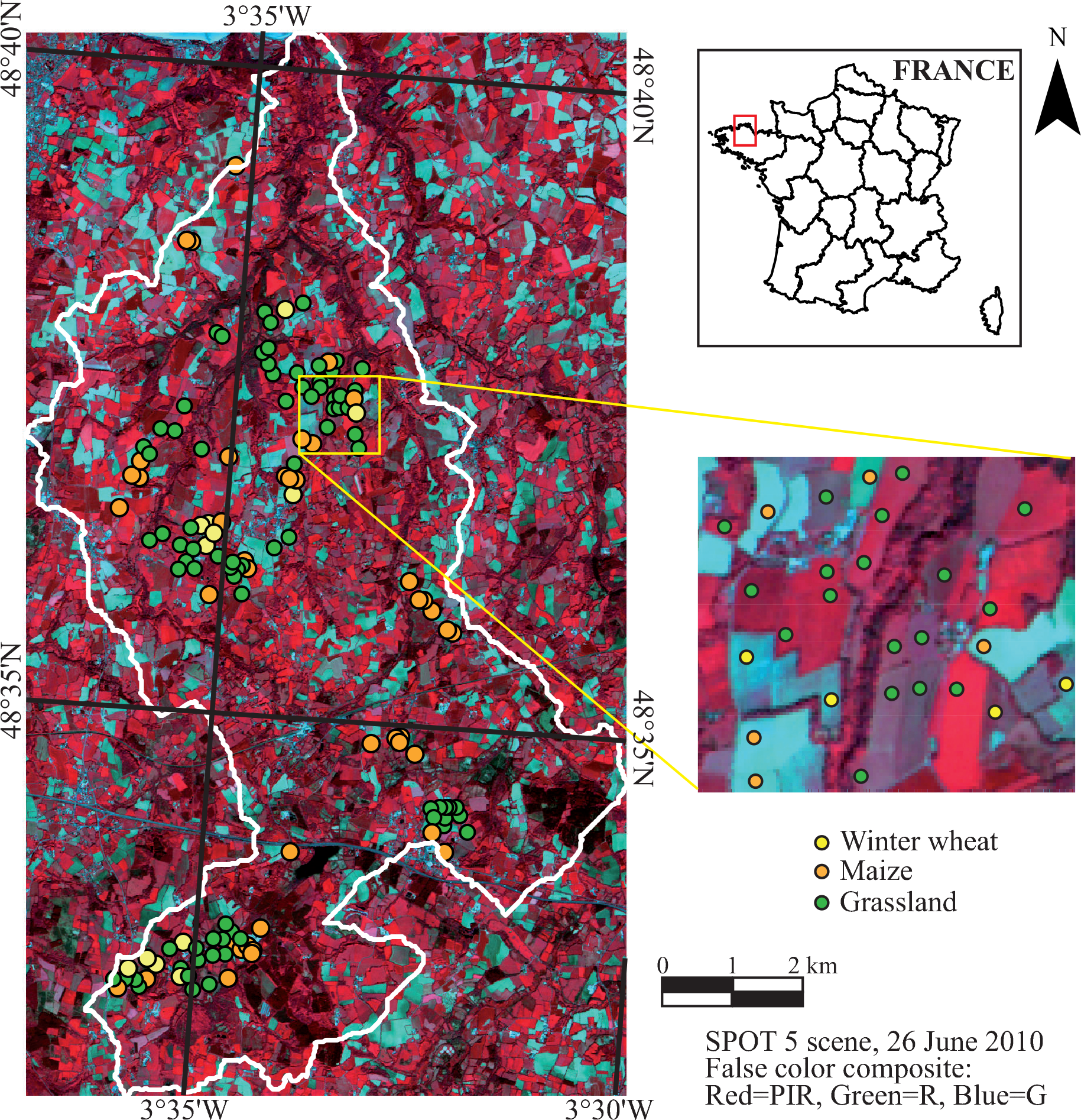
2.1. Site Description

The study was performed on a catchment area of 61.5 km2 located in central-north Brittany, France (Figure 1). Brittany has a moderate oceanic climate with mild winters and cool summers, high humidity and high mean cloudiness during the year. This study area, the Yar watershed, is characterized by relatively intensive farming, mainly oriented towards cattle production. Besides grassland, the main crops, maize and winter wheat, are produced in relation with industrial breeding. Thus, only these land cover classes, which occupy more than 95% of the arable land, were identified. High nitrogen rates in rivers, largely due to grassland regression and excessive fertilization on crops and grasslands, have been observed for several years on this site. This results in green algae development along the coast. Grasslands cover approximately 60% of the total vegetation area of the watershed and are distributed partly in wetlands (permanent grasslands) and partly in cultivated areas (temporary grasslands). Three types of grassland management practices are encountered in this area, namely grazing, mowing and mixed management (grazing and mowing). Thus, according to these farming practices, grassland fields can show a different vegetation status during the growing period.

2.2. Datasets

A series of nine satellite images with high/very high spatial resolution acquired in 2010 during the vegetation period were used for this study. Four cloud-free optical images acquired with SPOT-5 and Landsat sensors were used (Table 1).
In addition, fully polarimetric RADARSAT-2 images were acquired in ascending orbit and in fine quad-polarization mode (single look complex (SLC) products), thus presenting a nominal swath width of 25 km with a spatial resolution of 12 m (range) × 8 m (azimuth). The FQ18 (Fine Quad-Pol) beam that corresponds to a radar incidence angle of 37.56° was used. Five C-Band images (5405 GHz) were programmed from February 2010, to August 2010, over the study site (Table 2).
All acquired images were used to identify grasslands from crops, since grassland temporal profiles of biophysical or polarimetric variables are very different according to grassland management practices and, thus, can be very similar with crop temporal profiles of biophysical or polarimetric variables. Using multi-temporal optical and/or SAR data rather than one or two images per year should therefore improve grassland identification.
In parallel with image acquisition (with a difference of 1–5 days), field campaigns were conducted monthly during the growing season on the study site to calibrate and validate the classification of satellite images. An inventory of crop type was conducted on 236 fields (10% of the total number of the watershed fields) in 2010 during the time period of image acquisition. In addition to crop type, spectral signatures measured with an ASD FieldSpec-3 spectroradiometer [22,23] and hemispherical photographs [24] were recorded for 20 fields to derive NDVI and LAI values from these two types of data, respectively. Surveys were also conducted with volunteer farmers over four farms to describe the farming practices during the growing season.

3. Data Processing

3.1. Optical and SAR Data Preprocessing

In order to reduce errors resulting from instrumental variations in data acquisition, image noise and misregistration, the optical images were corrected from radiometric and atmospheric effects. These corrections were performed applying the 6S model (Second Simulation of a Satellite Signal in the Solar Spectrum vector code) developed by [25]. Then, geometric corrections were undertaken using ArcGIS 10. All data were georeferenced based on the Lambert 2 conformal conic system, the root mean square error being less than one pixel. Finally, the NDVI was calculated [26], and biophysical variables (LAI and fCOVER) were retrieved from satellite images using the PROSAIL (coupling of PROSPECT and SAIL models) radiative transfer model proposed by [27,28].
A 3 × 3 coherency matrix (T3) was firstly extracted from the raw Radarsat-2 images using PCI Geomatics© software. A Lee refined filter [29] was applied using a window of 3×3 pixels to reduce speckle noise. The images were then geocoded using the Shuttle Radar Topography Mission (SRTM) digital elevation model (DEM) to correct topographic deformations. The images were also geometrically corrected to the Lambert 2 conformal conic system using 40 ground control points selected from orthophoto images with a 0.5-m resolution. The geometric correction accuracy was less than one pixel. All polarizations in σ0 (dB) and intensity ratio (HH/VV, HH/HV and VV/VH) were firstly calculated from the 3 × 3 coherency matrix (T3) before applying two polarimetric decompositions in order to analyze the scattering mechanism of cropped vegetation: (1) the Freeman–Durden decomposition [20] to determine, for each pixel, the power contributions to total power due to double-bounce, volume and surface scattering; (2) the Cloude–Pottier decomposition [30], which is based on the eigenvector-eigenvalues decomposition of the coherence matrix, which computes the entropy (H, the incoherence degree of the dominant scatterer), the alpha angle, α, an angle between zero and 90 degrees (the identification of the type of scattering) and the Anisotropy, A (the amount of mixing between the second and third scattering mechanisms).
In total, fifteen types of variables were extracted from the satellite remote sensing images: three from optical images (NDVI, LAI and fCOVER) and twelve from SAR images (σ0HH, σ0VV, σ0HV, HH/VV, HH/HV, VV/HV, Freeman–Durden decomposition with double-bounce, volume and roughness and Cloude–Pottier decomposition with H, A, α). Since the remote sensing data used in this study have different spatial resolutions, variables derived from optical and SAR images that were calculated at pixel scale were computed at the field scale by applying the mean variable value within each field to the entire field. Field boundaries were delineated each year by photo-interpretation using the orthophotoplan and the satellite images. For each of these variables, temporal profiles were created: profiles derived from optical images include four points (four dates), while profiles derived from SAR images comprise five points (five dates).

3.2. Processing of Optical and SAR Data

3.2.1. Statistical Analysis

Optical and SAR variables have different intervals: for example, LAI ranges between zero and seven, NDVI ranges between zero and one, HH/VV range from 0.5 to 1.3, etc. Thus, in order to compare the temporal profiles extracted from the series of optical and SAR images and obtain independent data units, temporal profiles were normalized using the standard score according to the following equation:
z = x μ σ
where x is the temporal profile, μ is the mean and σ the standard deviation of the concerned profiles. Thus, a centered and reduced variable has a mean equal to zero and a standard deviation equal to one.
Then, in order to evaluate and compare the ability of the temporal profiles extracted from optical and polarimetric SAR data to discriminate grasslands from crops, transformed divergence (TD) was used. TD is a tool used to measure the separability between two profiles [31]. Firstly, the divergence (Dij) was computed according to Equation (2), and then, the TD ( D i j T) was calculated according to Equation (3).
D ij = 1 2 Tr { ( cov i cov j ) ( cov j 1 cov i 1 ) } + 1 2 Tr { ( cov i 1 + cov j 1 ) ( x ¯ i x ¯ j ) ( x ¯ i x ¯ j ) t }
where i and j are the profiles (of two classes) to compare, covi is the covariance matrix of profile i, i is the mean vector of signature i, Tr is the trace function and t is the transposition function.
D ij T = 2 ( 1 exp ( D ij 8 ) )
TD values, which can range from zero to two, decrease with increasing distances between classes. According to the empirical relationship between TD and the probability of correct classification [32]: classes can be separated with TD values greater than 1.9; classes can be fairly well separated with TD values between 1.7 and 1.9; and classes can be poorly separated with TD values below 1.7. TD can be computed for any combination of variables that are used to classify images and, thus, can be applied to a time series of remote sensing data.

3.2.2. Classification

According to TD analysis, the most discriminative optical and SAR variables were then selected and an SVM (support vector machine) procedure was performed to evaluate their ability to discriminate grasslands from crops. Well-known SVM techniques [33,34] are able to efficiently classify a set of data where the separability between classes is not obvious (the main idea consists in performing a projection of all data onto a specific space where the separability is higher). To evaluate classification performance, 2/3 of the 236 sample fields were used for training and 1/3 for validation. Fifteen percent of the validation set corresponds to winter wheat fields, 22% to maize and 63% to grassland fields. Classification accuracy was assessed using the kappa index (K) and the overall accuracy [35].

4. Results and Discussion

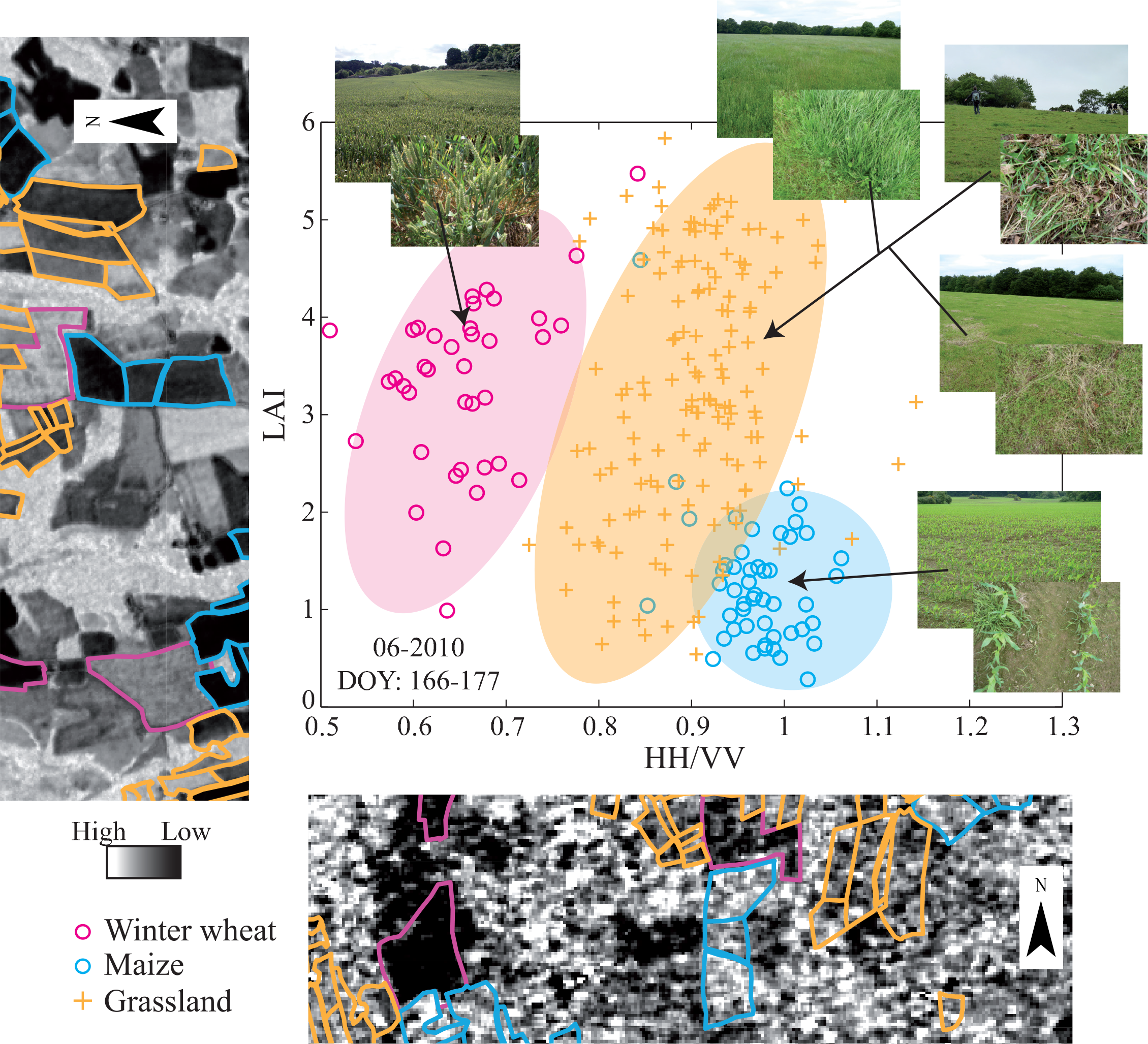
4.1. Analysis of Class Separability

The transformed divergence values between the three land cover classes (winter wheat, maize and grassland) calculated from the temporal profiles of variables derived from optical and SAR images are given in Table 3. The variable sets included three optical variables and in terms of SAR variables: three single polarizations, one combination of polarizations, three polarization ratios and two polarimetric decomposition parameters. It can be observed that TD values are very high (TD ≥ 1.9), indicating that the land cover classes have very good separability for any of the optical and SAR variables. The use of time series of remotely sensed data allows plant growth to be monitored and winter wheat and maize to be discriminated from grasslands.
Regarding the TD values obtained with temporal profiles of variables derived from optical images, the biophysical variables are the most accurate for the discrimination of the three land cover classes. It is related to the fact that NDVI is sensitive to the soil contribution and to the atmosphere [36,37]. Moreover, some NDVI differences are caused by sensor-specific relative spectral response functions [38]. In addition, it was shown that for a vegetation cover rate above 60%, vegetation indices using the NIR spectral band are insensitive to changes related to vegetation [39,40]. On the other hand, biophysical parameters have been proven to be very efficient and suitable for vegetation monitoring [7,10,41,42]. The TD values of LAI are the highest, showing that the temporal evolution of LAI is indeed informative about vegetation growth, density and land management practices [43,44]. The TD values for fCOVER are slightly lower. Moreover, TD values between winter wheat and grassland are a bit lower for NDVI temporal profiles than for LAI temporal profiles. Thus, we suggest relying on LAI series to discriminate grasslands from the two other land cover classes.
Concerning SAR variables, the combination of polarizations (HH, VV, HV, VH) and the two polarimetric decompositions (Freeman–Durden and Cloude–Pottier) show a TD value of 2.0, which is consistent with numerous studies showing the interest of radar polarimetric information for land cover monitoring [1820]. Moreover, polarimetric information is well correlated with vegetation status [1214,16]. Thus, the classification process was performed using these three variable sets.

4.2. Analysis of Temporal Variables Used for Classification

4.2.1. LAI and HH/VV Variables Extracted from Optical and SAR Data, Respectively

Field temporal profiles of LAI and the HH/VV polarization ratio are illustrated in Figure 2 for the three land cover classes. LAI provides information on vegetation growth and status, and the HH/VV polarization ratio indirectly provides information on agricultural practices [17]. Indeed, in C-band, σ0 HH is generally higher than that of σ0 VV, because of the stronger attenuation of VV backscattering by vertical stems [13,45,46]. Backscattering coefficients are thus strongly linked to the phenology of the crop, which influences the scattering mechanisms of the target [1214]. Thus, numerous studies use a multitemporal HH/VV ratio for land use and land cover monitoring in agricultural areas [17,47,48].
Land cover classes show very different profiles based on the agricultural calendar (Figure 3) reflecting farming practices:
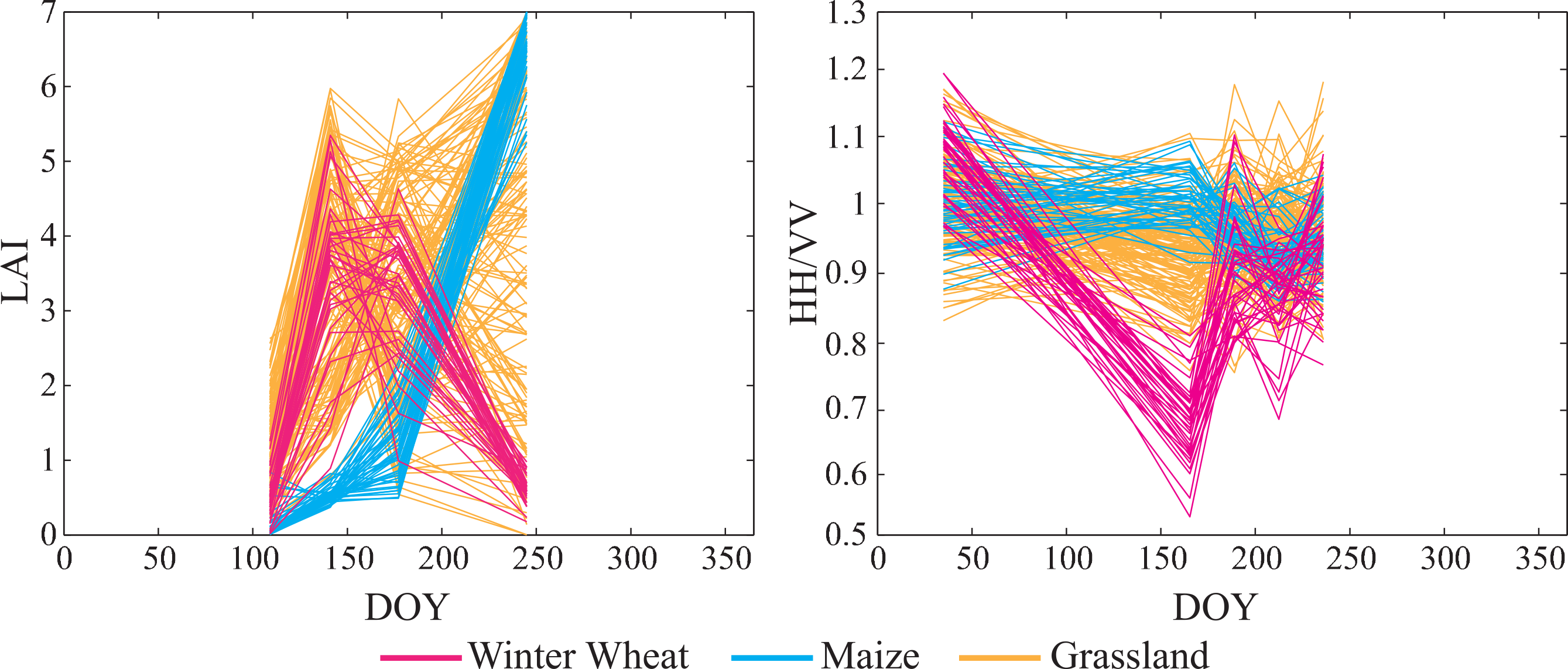
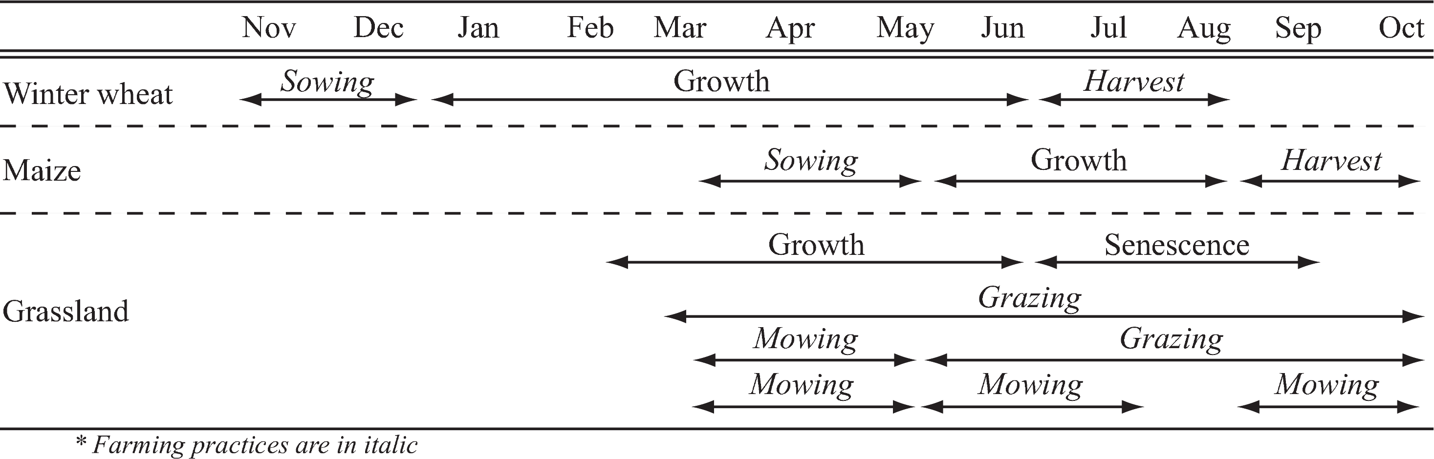
  • The LAI profiles for the winter wheat illustrate the growth period from leaf development to flowering (May (DOY: 141) and June (DOY: 177) images) with LAI values higher than three followed by harvest after senescence at the end of the summer period (DOY: 245) with values lower than one. HH/VV ratios show values close to one at the beginning of leaf development (February (DOY: 33)), which highlights few backscattering variations between HH and VV due to the low development of winter wheat during this period (specular scattering). On the other hand, at the flowering stage during the spring period (June (DOY: 166)), values are comprised between 0.5 and 0.8, illustrating high levels of surface roughness explained by the growth of plants (low values of backscattering coefficient VV due to vegetation growth). At the senescence stage (July (DOY: 190)), the harvest begins and the ratio values increase. In early August (DOY: 214), the decrease of HH/VV ratio values can be explained by vegetation regrowth, while at the end of August (DOY: 238), the increase of HH/VV ratio values is related to the plowing of winter wheat.
  • LAI profiles of maize illustrate bare soil and a sowing period lasting until the end of June (DOY: 177) followed by the growth period from leaf development to ripening until September (DOY: 245). The HH/VV ratio values appear very heterogeneous during the winter period in February (DOY: 33). At this time period, maize has not yet been sown (sowing in April), and before this crop, different land use and land cover practices (labor, intercrop, etc.) can be observed associated with very different scattering mechanisms. In June (DOY: 166), the HH/VV ratio values are high (between 0.9 and 1.1), showing different dominant scattering mechanisms for each polarization corresponding to leaf development (maize growth). During stem elongation and flowering in July (DOY: 190) and August (DOY: 214 and 238), maize HH/VV ratio values are lower (between 0.8 and one), because of the presence of a high level of vegetation cover during this period (diffuse scattering).
  • LAI profiles of grasslands show several shapes according to farming practices. We can observe high LAI values during the growth period (from leaf development to flowering), from April to June, whereas after this time period, LAI values decrease at varying rates according to grassland management practices. Indeed, three farming practices can be identified within the grassland class: grazing, mowing and mixed management. A strong decrease in LAI values can be observed after inflorescence emergence in June (DOY: 177) for mown fields, while LAI values decrease more slowly for grazed fields. After the end of the summer period, in September (DOY: 245), two different LAI scenarios are observed for mowed fields according to the ripening stage: some of them were recently mowed; thus, the LAI values are very low (less than one); and some of them were not yet mowed and showed very high LAI values (more than five). Grazing occurred during the growing season after stem elongation. The HH/VV ratio profiles of grassland management were characterized by high variance for each date, and grazing, mowing and mixed management in grasslands could not be exactly discriminated.
Temporal profiles allow land cover classes to be discriminated, while values of the considered variables are similar on some dates. The growth status of different crops can be similar on some time periods. Furthermore, some dissimilarities can be observed between values of the three land cover classes during the month of June (DOY 166 for LAI and 177 for HH/VV ratio); thus, it appears to be the best time period when optical and SAR data are combined. LAI values of maize are much smaller than those of grassland and winter wheat, while the HH/VV ratio values of winter wheat class are smaller than those of maize and grassland (Figure 2). Therefore, the three land cover classes can be discriminated using the combination of LAI and HH/VV ratio values.
Figure 4 is the scatter plot of the field samples of the three land cover classes considered in a space comprising the HH/VV polarization ratio and the LAI variable for June, 2010, the only month during this study in which optical and SAR data were acquired. The three land cover classes were well discriminated by the HH/VV and LAI combination. In June, values for winter wheat class were quite unique in that the HH/VV polarization ratio values were much smaller than those for the other classes (<0.8, attenuation of the backscattering coefficient in VV polarization), while LAI values were similar to those of the grassland class. The maize HH/VV polarization ratio values were generally much higher than those from the other classes (>0.9, a similar backscattering coefficient for the two polarizations due to bare soil contribution), but a limited number of grassland fields showed the same HH/VV values. Thus, by the combination of the June HH/VV ratio and LAI values, maize identification was achieved with small LAI values (<2) and high HH/VV values (>0.9). Grassland can be discriminated from winter wheat with HH/VV ratio values comprised between 0.8 and 0.9 (winter wheat HH/VV ratio values are comprised between 0.5 and 0.8). Grassland can be discriminated from maize with (1) LAI values comprised between zero and two and HH/VV ratio values comprised between 0.8 and 0.9 or with (2) LAI values higher than two (maize LAI values are smaller than two and HH/VV ratio values are higher than 0.9).

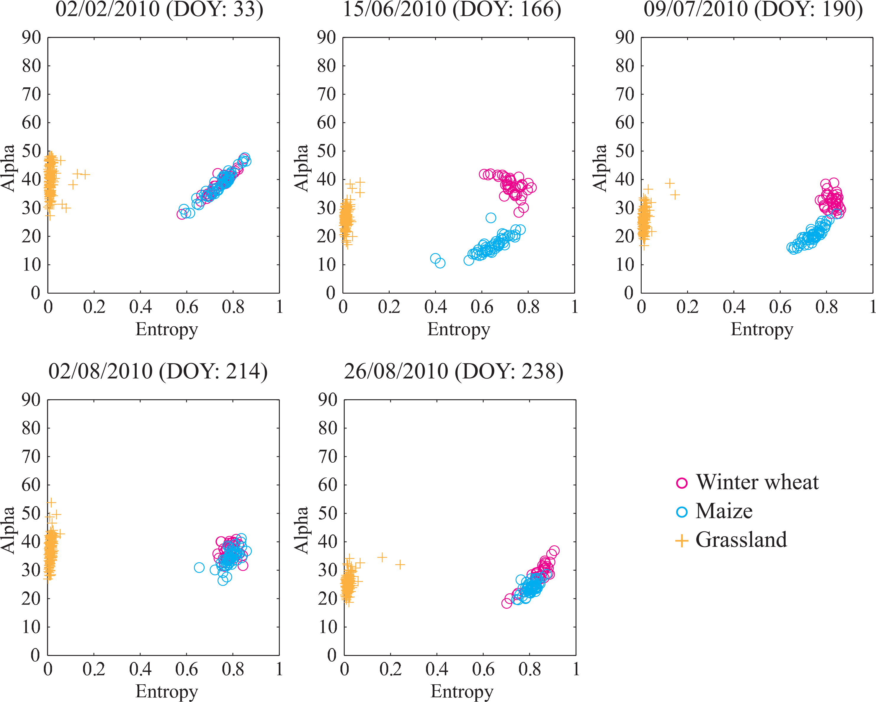
4.2.2. Entropy and Alpha Polarimetric Variables Extracted from SAR Data

Illustrated in Figure 5, winter wheat, maize and grassland field samples were then plotted for each acquisition date in the data space of the entropy and alpha polarimetric variables, which represent scattering mechanisms defined by [30]. The Cloude–Pottier representation (H, α) helps to define the dominant type of scattering: multiple, volume or surface. Alpha angle (α) values are comprised between 0° and 90°, with 0° indicating dominant smooth scattering, 45° a dominant volume or dipolar scattering and 90° diffuse scattering (or dihedral). When the entropy variable (H) is equal to zero, only one scattering dominant mechanism occurs compared to several scattering mechanisms if H = 1. Figure 5 shows a very good separability between the three land cover classes, particularly in June. This figure also highlights that it is necessary to use multi-temporal data to identify these classes, since depending on the acquisition date, winter wheat and maize show similarities (DOY: 33, 214 and 238) and, thus, cannot be discriminated using only these dates (as seen previously with temporal profiles (Figure 4) and the agricultural calendar (Figure 3)). The temporal variation of radar response has proven to be effective for land cover monitoring, varying according to vegetation growth to the saturation level. Indeed, as shown by [13] or [49], saturation can be observed with radar backscattering on sugar cane or rice with a crop height higher than 50 cm. We can observe this phenomenon on maize and winter wheat fields from August when maize and winter wheat show similar values (Figure 5). Thus, the use of multi-temporal data is interesting for crop monitoring. Generally, grasslands show lower entropy values (comprised between zero and 0.2) than winter wheat and maize classes (H values comprised between 0.6 and 0.9) that are characterized by different scattering mechanisms (surface, double-bounce, etc.). Moreover, June and July appear to be the most appropriate time period to distinguish winter wheat from maize. We observed that winter wheat have higher α values than maize, from 30 to 45 and from 10 to 25, respectively, which indicates a dominant volume scattering for winter wheat and a smoother surface scattering contribution for maize in June. According to the diagram of the bi-dimensional classification based on the entropy (H) and orientation alpha angle (α) from [30,50], during these two months, the dominant scattering mechanisms for winter wheat is the volume with a medium entropy and the dominant scattering mechanisms for maize is the surface with a medium entropy [51,52]. Maize fields are just being sown at this period; thus, bare soil is dominant while winter wheat fields are already growing. Concerning grasslands, the dominant scattering mechanism is the surface with a very low entropy. Moreover, according to [30], low values of entropy (H < 0.5) are of less interest and provide fewer details on the class. Thus, it appears that SAR can be very useful in classifying the three considered land cover classes of interest.

4.3. Classification

Tables 4 and 7 show the confusion matrices of the land cover classifications using optical or SAR variables. Globally, land cover classes are well separated: classifications using Freeman–Durden decomposition parameters (Table 6) or Cloude–Pottier decomposition parameters (Table 7) produced the highest overall accuracy (OA) and kappa values (K) with 97% OA, K = 0.95 and 99% OA, K = 0.98, respectively. Classifications using the LAI variable (Table 4) show an overall accuracy of 88% and a kappa value of 0.81. Misclassification errors can be observed between winter wheat and grassland classes, as previously detailed and illustrated in Figure 6, these two classes showing similar LAI temporal profiles during the vegetation development stage (Figures 2 and 3). Moreover, only four optical images were used in this study, because of cloud cover during the summer period; thus, some information about vegetation status is missing. Concerning classifications using SAR variables, the combination of polarizations (Table 5) show an overall accuracy of 96% and a kappa value of 0.87. We observe an underestimation of 17% of winter wheat in favor of the grassland class and an underestimation of 2% of grassland in favor of the maize. The classification results using Freeman–Durden decomposition parameters (Table 6) and Cloude–Pottier decomposition parameters (Table 7) show some misclassification between winter wheat and maize, while grassland fields are very well separated.
Tables 8 and 10 shows the confusion matrices of land cover classifications using the combination of optical and SAR data. Land cover classes are very well separated (100% accuracy) with the combination of LAI Freeman–Durden decomposition parameters and LAI Cloude–Pottier decomposition parameters. The combination of optical and SAR data eliminated misclassification errors. Thus, four optical images and five SAR images distributed throughout the year are enough to discriminate winter wheat, maize and grassland. Moreover, the use of polarimetric decomposition, such as Freeman–Durden or Cloude–Pottier, in addition to LAI, remove possible misclassification errors between land cover classes, as shown by [12]. Furthermore, polarimetric data, such as Radarsat-2, can be very useful to discriminate crops in addition to optical data [51].

5. Conclusions

In this study, we have evaluated the ability of optical and/or SAR time series images to discriminate between grasslands and crops in agricultural areas where cloud cover is very high most of the time. We showed that among a series of variables derived from multi-temporal images acquired with optical and SAR sensors, LAI and Freeman–Durden and Cloude–Pottier polarimetric decompositions were proven to be the best optical and SAR variables, respectively, to identify grasslands. We also highlight that (i) the classification accuracy of SAR variables alone is higher than that of optical variables alone (K: 0.98 compared to 0.81); (ii) classification using Cloude–Pottier decomposition parameters shows a higher accuracy than that using the combination of polarizations HH, VV and HV and the Freeman–Durden decomposition parameters (K: 0.98 compared to 0.87 and 0.95, respectively); and (iii) the combination of the LAI variable and SAR decomposition parameters (Freeman–Durden and Cloude–Pottier) allow grassland to be discriminated from cropland with an accuracy of 100%. As a perspective, this approach could be applied to multi-annual SAR and optical time series to identify grassland removal and, thus, to monitor grassland inter-annual dynamics and to define their status in farming systems. Furthermore, in the context of upcoming sensors Sentinel-1, Sentinel-2 or Venμs, a large amount of satellite images with high spatial and temporal resolutions will be soon available, offering new perspectives for intra-annual grassland monitoring. Some grassland farming practices, such as grazing, mowing and fertilizing, as well as their intensity, could be investigated using the synergy of remotely sensed optical and SAR time series. This method, based on the use of temporal profiles derived from optical and SAR data, can be extended to other regions to monitor areas with similar characteristics and same land cover classes, as well as to identify other land cover types. The main requirement is that time series of satellite images should be acquired during the vegetation growing period. Moreover, in parallel with image acquisition, field campaigns should be conducted to assess image classification accuracy.

Acknowledgments

This work was supported by the National Agency for Research (ANR) SYSTERRA-ACASSYA (Supporting the agro ecological evolution of breeding systems in coastal watersheds) program (ANR-08-STRA-01). We would also like to thank the National Centre for Space Studies (CNES) for providing us with the optical satellite images, Vigisat-CLS (Collecte Localisation Satellites)S for providing us with the SAR data, Sally Ferguson for revising the manuscript and the anonymous referees for their valuable comments.

Author Contributions

All authors contributed extensively to the work presented in this paper. Pauline Dusseux and Samuel Corgne processed the optical and radar images and conducted the field work. All authors led an interpretation of the results and drafted the manuscript. Laurence Hubert-Moy and Thomas Corpetti initiated the project, which was revised by all authors. All authors read and approved the final manuscript.

Conflicts of Interest

The authors declare no conflicts of interest.

References

  1. Lobell, D.B.; Field, C.B. Global scale climate-crop yield relationships and the impacts of recent warming. Environ. Res. Lett 2007, 2, 014002. [Google Scholar] [CrossRef]
  2. Batáry, P.; Báldi, A.; Erdõs, S. Grassland versus non-grassland bird abundance and diversity in managed grasslands: Local, landscape and regional scale effects. Biodivers. Conserv 2007, 16, 871–881. [Google Scholar]
  3. Vertès, F.; Hatch, D.; Velthof, G.; Taube, F.; Laurent, F.; Loiseau, P.; Recous, S. Short-Term and Cumulative Effects of Grassland Cultivation on Nitrogen and Carbon Cycling in Ley-Arable Rotations. Proceedings of 14th Symposium of the Grassland Science in Europe, Permanent and Temporary Grassland: Plant, Environment and Economy, Gent, Belgium, 3–5 September 2007; pp. 227–246.
  4. Arrouays, D.; Deslais, W.; Badeau, V. The carbon content of topsoil and its geographical distribution in France. Soil Use Manag 2001, 17, 7–11. [Google Scholar]
  5. Peeters, A. Importance, evolution, environmental impact and future challenges of grasslands and grassland-based systems in Europe. Grassl. Sci 2009, 55, 113–125. [Google Scholar]
  6. Poudevigne, I.; Alard, D. Landscape and agricultural patterns in rural areas: A case study in the Brionne Basin, Normandy, France. J. Environ. Manag 1997, 50, 335–349. [Google Scholar]
  7. Jacquemoud, S.; Verhoef, W.; Baret, F.; Bacour, C.; Zarco-Tejada, P.; Asner, G.; François, C.; Ustin, S. PROSPECT + SAIL models: A review of use for vegetation characterization. Remote Sens. Environ 2009, 113, S56–S66. [Google Scholar]
  8. Rondeaux, G.; Steven, M.; Baret, F. Optimization of soil-adjusted vegetation indices. Remote Sens. Environ 1996, 55, 95–107. [Google Scholar]
  9. Gao, S.; Niu, Z.; Huang, N.; Hou, X. Estimating the Leaf Area Index, height and biomass of maize using HJ-1 and RADARSAT-2. Int. J. Appl. Earth Obs. Geoinf 2013, 24, 1–8. [Google Scholar]
  10. Friedl, M.; Schimel, D.; Michaelsen, J.; Davis, F.W.; Walker, H. Estimating grassland biomass and Leaf Area Index using ground and satellite data. Int. J. Remote Sens 1994, 15, 1401–1420. [Google Scholar]
  11. Wei, X. Biomass estimation: A remote sensing approach. Geogr. Compass 2010, 4, 1635–1647. [Google Scholar]
  12. McNairn, H.; Brisco, B. The application of C-band polarimetric SAR for agriculture: A review. Can. J. Remote Sens 2004, 30, 525–542. [Google Scholar]
  13. Baghdadi, N.; Boyer, N.; Todoroff, P.; El Hajj, M.; Bégué, A. Potential of SAR sensors TerraSAR-X, ASAR/ENVISAT and PALSAR/ALOS for monitoring sugarcane crops on Reunion Island. Remote Sens. Environ 2009, 113, 1724–1738. [Google Scholar]
  14. Inoue, Y.; Sakaiya, E.; Wang, C. Capability of C-band backscattering coefficients from high-resolution satellite SAR sensors to assess biophysical variables in paddy rice. Remote Sens. Environ 2014, 140, 257–266. [Google Scholar]
  15. Bouman, B.A.M. Crop parameter estimation from ground-based x-band (3-cm wave) radar backscattering data. Remote Sens. Environ 1991, 37, 193–205. [Google Scholar]
  16. Le Toan, T.; Beaudoin, A.; Riom, J.; Guyon, D. Relating forest biomass to SAR data. IEEE Trans. Geosci. Remote Sens 1992, 30, 403–411. [Google Scholar]
  17. Liu, C.; Shang, J.; Vachon, P.; McNairn, H. Multiyear crop monitoring using polarimetric RADARSAT-2 data. IEEE Trans. Geosci. Remote Sens 2013, 51, 2227–2240. [Google Scholar]
  18. Buckley, J.; Smith, A. Monitoring Grasslands with Radarsat 2 Quad-Pol Imagery. Proceedings of IEEE International Geoscience and Remote Sensing Symposium, IGARSS ’10, Honolulu, HI, USA, 25–30 July 2010; pp. 3090–3093.
  19. Smith, A.M.; Buckley, J.R. Investigating RADARSAT-2 as a tool for monitoring grassland in western Canada. Can. J. Remote Sens 2011, 37, 93–102. [Google Scholar]
  20. Freeman, A.; Villasenor, J.; Klein, J.; Hoogeboom, P.; Groot, J. On the use of multi-frequency and polarimetric radar backscatter features for classification of agricultural crops. Int. J. Remote Sens 1994, 15, 1799–1812. [Google Scholar]
  21. Dusseux, P.; Hubert-Moy, L.; Lecerf, R.; Gong, X.; Corpetti, T. Identification of Grazed and Mown Grasslands Using a Time Series of High-Spatial-Resolution Remote Sensing Images. Proceedings of 6th International Workshop on the Analysis of Multi-temporal Remote Sensing Images (Multi-Temp), Trento, Italy, 12–14 July 2011; pp. 145–148.
  22. ASD. FieldSpec 3 Portable Spectroradiometer User’s Guide; Analytical Spectral Devices: Boulder, CO, USA, 2000. [Google Scholar]
  23. Lillesand, T.; Kiefer, R.; Chipman, J. Remote Sensing and Image Interpretation, 6th ed.; John Wiley ans Sons: Toronto, ON, Canada, 2008; p. 768. [Google Scholar]
  24. Weiss, M.; Baret, F.; Smith, G.J.; Jonckheere, I.; Coppin, P. Review of methods for in situ Leaf Area Index (LAI) determination: Part II. Estimation of LAI, errors and sampling. Agric. For. Meteorol 2004, 121, 37–53. [Google Scholar]
  25. Vermote, E.; Tanre, D.; Deuze, J.; Herman, M.; Morcette, J.J. Second simulation of the satellite signal in the solar spectrum, 6S: An overview. IEEE Trans. Geosci. Remote Sens 1997, 35, 675–686. [Google Scholar]
  26. Rouse, J.; Haas, R.; Schell, J.; Deering, D.; Harlan, J. Monitoring the Vernal Advancement of Retrogradation of Natural Vegetation; Type III, Final report; NASA/GSFC: Greenbelt, MD, USA, 1974; p. 371. [Google Scholar]
  27. Jacquemoud, S.; Baret, F. PROSPECT: A model of leaf optical properties spectra. Remote Sens. Environ 1990, 34, 75–91. [Google Scholar]
  28. Verhoef, W. Light scattering by leaf layers with application to canopy reflectance modeling: The SAIL model. Remote Sens. Environ 1984, 16, 125–141. [Google Scholar]
  29. Lee, J.; Grunes, M.; de Grandi, G. Polarimetric SAR speckle filtering and its implication for classification. IEEE Trans. Geosci. Remote Sens 1999, 37, 2363–2373. [Google Scholar]
  30. Cloude, S.; Pottier, E. An entropy based classification scheme for land applications of polarimetric SAR. IEEE Trans. Geosci. Remote Sens 1997, 35, 68–78. [Google Scholar]
  31. Richards, J.A. Remote Sensing Digital Image Analysis: An Introduction, 5th ed.; Springer: New Jersey, NJ, USA, 2012; p. 494. [Google Scholar]
  32. Swain, P.H.; King, R.C. Two Effective Feature Selection Criteria for Multispectral Remote Sensing. Proceedings of the First International Joint Conferences on Pattern Recognition, Washington, DC, USA; 1973; pp. 536–540. [Google Scholar]
  33. Zhang, T. An introduction to support vector machines and other Kernel-based learning methods. AI Mag 2001, 22, 103–104. [Google Scholar]
  34. Burges, C.J.C. A tutorial on support vector machines for pattern recognition. Data Min. Knowl. Discov 1998, 2, 121–167. [Google Scholar]
  35. Congalton, R.G. A review of assessing the accuracy of classifications of remotely sensed data. Remote Sens. Environ 1991, 37, 35–46. [Google Scholar]
  36. Henebry, G.M. Detecting change in grasslands using measures of spatial dependence with Landsat TM data. Remote Sens. Environ 1993, 46, 223–234. [Google Scholar]
  37. Baret, F.; Guyot, G. Potentials and limits of vegetation indices for LAI and APAR assessment. Remote Sens. Environ 1991, 35, 161–173. [Google Scholar]
  38. Franke, J.; Heinzel, V.; Menz, G. Assessment of NDVI- Differences Caused by Sensor Specific Relative Spectral Response Functions. Proceedings of IEEE International Geoscience and Remote Sensing Symposium, Denver, CO, USA, 31 July–4 August 2006; pp. 1138–1141.
  39. Gitelson, A.A.; Kaufman, Y.J.; Stark, R.; Rundquist, D. Novel algorithms for remote estimation of vegetation fraction. Remote Sens. Environ 2002, 80, 76–87. [Google Scholar]
  40. Glenn, E.P.; Huete, A.R.; Nagler, P.L.; Nelson, S.G. Relationship between remotely-sensed vegetation indices, canopy attributes and plant physiological processes: What vegetation indices can and cannot tell us about the landscape. Sensors 2008, 8, 2136–2160. [Google Scholar]
  41. Zhang, C.; Guo, X. Monitoring northern mixed prairie health using broadband satellite imagery. Int. J. Remote Sens 2008, 29, 2257–2271. [Google Scholar]
  42. Guo, X.; Price, K.P.; Stiles, J.M. Biophysical and spectral characteristics of cool- and warm-season grasslands under three land management practices in Eastern Kansas. Nat. Resour. Res 2000, 9, 321–331. [Google Scholar]
  43. Asam, S.; Fabritius, H.; Klein, D.; Conrad, C.; Dech, S. Derivation of Leaf Area Index for grassland within alpine upland using multi-temporal RapidEye data. Int. J. Remote Sens 2013, 34, 8628–8652. [Google Scholar]
  44. Chen, J.M.; Black, T.A. Measuring Leaf Area Index of plant canopies with branch architecture. Agric. For. Meteorol 1991, 57, 1–12. [Google Scholar]
  45. Ribbes, F. Rice field mapping and monitoring with RADARSAT data. Int. J. Remote Sens 1999, 20, 745–765. [Google Scholar]
  46. Le Toan, T.; Ribbes, F.; Wang, L.; Floury, N.; Ding, K.; Kong, J.; Fujita, M.; Kurosu, T. Rice crop mapping and monitoring using ERS-1 data based on experiment and modeling results. IEEE Trans. Geosci. Remote Sens 1997, 35, 41–56. [Google Scholar]
  47. Betbeder, J.; Rapinel, S.; Corpetti, T.; Pottier, E.; Corgne, S.; Hubert-Moy, L. Multi-temporal classification of TerraSAR-X data for wetland vegetation mapping. Proc. SPIE 2013, 8887. [Google Scholar] [CrossRef]
  48. Koppe, W.; Gnyp, M.L.; Hütt, C.; Yao, Y.; Miao, Y.; Chen, X.; Bareth, G. Rice monitoring with multi-temporal and dual-polarimetric TerraSAR-X data. Int. J. Appl. Earth Obs. Geoinf 2013, 21, 568–576. [Google Scholar]
  49. Lam-Dao, N.; Le Toan, T.; Apan, A.; Bouvet, A.; Young, F.; Le-Van, T. Effects of changing rice cultural practices on C-band synthetic aperture radar backscatter using Envisat advanced synthetic aperture radar data in the Mekong River Delta. J. Appl. Remote Sens 2009, 3, 033563:1–033563:17. [Google Scholar]
  50. Lee, J.; Pottier, E. Polarimetric Radar Imaging: From Basics to Applications; CRC Press: New York, NY, USA, 2009; p. 422. [Google Scholar]
  51. McNairn, H.; Shang, J.; Jiao, X.; Champagne, C. The contribution of ALOS PALSAR multipolarization and polarimetric data to crop classification. IEEE Trans. Geosci. Remote Sens 2009, 47, 3981–3992. [Google Scholar]
  52. Park, S.E.; Moon, W. Unsupervised classification of scattering mechanisms in polarimetric SAR sata using fuzzy logic in entropy and Alpha Plane. IEEE Trans. Geosci. Remote Sens 2007, 45, 2652–2664. [Google Scholar]
Figure 1. Location of the study site and field data locations.
Remotesensing 06 06163f1
Figure 2. Field temporal profiles of the LAI variable and HH/VV polarization ratio.
Remotesensing 06 06163f2
Figure 3. Phenology stages and farming practices for the three land cover classes.
Remotesensing 06 06163f3
Figure 4. Scatter plot of the field samples of the three land cover classes in a space comprising the HH/VV polarization ratio and the LAI variable for June 2010 (satellite images: DOY 166 for the HH/VV ratio and DOY 177 for the LAI variable).
Remotesensing 06 06163f4
Figure 5. Scatter plot of the three land cover classes in the space of the entropy (H) and alpha (α) variables derived from Cloude–Pottier decomposition for each SAR acquisition date.
Remotesensing 06 06163f5
Figure 6. Illustration of classification results: extract of the study site of misclassified fields using the LAI variable or Cloude–Pottier decomposition parameters and well classified fields using a combination of LAI and Cloude–Pottier decomposition parameters.
Remotesensing 06 06163f6
Table 1. Characteristics of optical satellite images.
Date (DOY) (Days of the Year)SensorSpatial Resolution (m)Spectral Bands*
April 19, 2010 (109)SPOT 55 × 5G, R, NIR
May 21, 2010 (141)SPOT 510 × 10G, R, NIR
June 26, 2010 (177)SPOT 55 × 5G, R, NIR
September 2, 2010 (245)Landsat TM530 × 30B, G, R, NIR, SWIR
*B = blue, G = green, R = red, NIR = near-infrared and SWIR = short-wavelength infrared.
Table 2. Characteristics of Radarsat-2 images.
Spatial Resolution12 × 12 m
Azimuth Resolution8m
PolarizationFull (HH, VV, HV, VH)
ModeFine Quad-Pol
Incidence Angle37.56° (Right Ascending)
Coverage25 km × 25 km
Dates (DOY) (Days of the Year)2 February 2010 (33)
15 June 2010 (166)
9 July 2010 (190)
2 August 2010 (214)
26 August 2010 (238)
Table 3. Transformed divergence values between the land cover classes for optical and SAR variables.
Variable Set
Winter Wheat-MaizeWinter Wheat-GrasslandMaize-Grassland
Land Cover
Optical VARIABLES
NDVI2.001.871.99
LAI2.001.992.00
fCOVER2.001.972.00

SAR VARIABLES

Single polarization
σ0HH1.911.992.00
σ0VV1.952.001.98
σ0HV1.981.921.86
Combination of polarizations
HH, VV, HV2.002.002.00
Polarization ratio
HH/VV2.002.001.90
HH/HV1.922.001.99
VV/HV2.002.001.70
Polarimetric decomposition
Freeman–Durden2.002.002.00
Cloude–Pottier2.002.002.00
Table 4. Confusion matrix (in %) for land cover classification using the LAI variable derived from four optical images.
Winter WheatMaizeGrasslandTotal
Winter wheat8301422
Maize0100022
Grassland1708656
Total100100100100
Overall accuracy = 88%, kappa index = 0.81.
Table 5. Confusion matrix (in %) for land cover classification using a combination of polarizations, HH, VV and HV computed from five SAR images.
Winter WheatMaizeGrasslandTotal
Winter wheat830013
Maize0100223
Grassland1709864
Total100100100100
Overall accuracy = 96%, kappa index = 0.87.
Table 6. Confusion matrix (in %) for land cover classification using the Freeman–Durden decomposition parameters computed from five SAR images.
Winter WheatMaizeGrasslandTotal
Winter wheat830013
Maize17100024
Grassland0010063
Total100100100100
Overall accuracy = 97%, kappa index = 0.95.
Table 7. Confusion matrix (in %) for land cover classification using the Cloude–Pottier decomposition parameters computed from five SAR images.
Winter WheatMaizeGrasslandTotal
Winter wheat920014
Maize8100023
Grassland0010063
Total100100100100
Overall accuracy = 99%, kappa index = 0.98.
Table 8. Confusion matrix (in %) for land cover classification using a combination of optical and SAR variables: LAI and HH, VV, HV.
Winter WheatMaizeGrasslandTotal
Winter wheat920215
Maize0100022
Grassland809863
Total100100100100
Overall accuracy = 97%, kappa index = 0.94.
Table 9. Confusion matrix (in %) for land cover classification using a combination of optical and SAR variables: LAI and Freeman–Durden decomposition parameters.
Winter WheatMaizeGrasslandTotal
Winter wheat1000015
Maize0100022
Grassland0010063
Total100100100100
Overall accuracy = 100%, kappa index = 1.
Table 10. Confusion matrix (in %) for land cover classification using a combination of optical and SAR variables: LAI and Cloude–Pottier decomposition parameters.
Winter WheatMaizeGrasslandTotal
Winter wheat1000015
Maize0100022
Grassland0010063
Total100100100100
Overall accuracy = 100%, kappa index = 1.

