A Comparison of Advanced Regression Algorithms for Quantifying Urban Land Cover

Abstract

Quantitative methods for mapping sub-pixel land cover fractions are gaining increasing attention, particularly with regard to upcoming hyperspectral satellite missions. We evaluated five advanced regression algorithms combined with synthetically mixed training data for quantifying urban land cover from HyMap data at 3.6 and 9 m spatial resolution. Methods included support vector regression (SVR), kernel ridge regression (KRR), artificial neural networks (NN), random forest regression (RFR) and partial least squares regression (PLSR). Our experiments demonstrate that both kernel methods SVR and KRR yield high accuracies for mapping complex urban surface types, i.e., rooftops, pavements, grass- and tree-covered areas. SVR and KRR models proved to be stable with regard to the spatial and spectral differences between both images and effectively utilized the higher complexity of the synthetic training mixtures for improving estimates for coarser resolution data. Observed deficiencies mainly relate to known problems arising from spectral similarities or shadowing. The remaining regressors either revealed erratic (NN) or limited (RFR and PLSR) performances when comprehensively mapping urban land cover. Our findings suggest that the combination of kernel-based regression methods, such as SVR and KRR, with synthetically mixed training data is well suited for quantifying urban land cover from imaging spectrometer data at multiple scales.

1. Introduction

Urban areas represent highly challenging environments for remote sensing data analysis. Compared to natural environments, urban areas are very heterogeneous featuring a high spectral diversity of various anthropogenic and natural materials [1,2] and a spatially complex, three-dimensional surface geometry [3,4]. To separate meaningful impervious and vegetation sub-categories on a purely spectral basis [5,6], imaging spectrometer data is often the only adequate source. Results in [7,8] illustrate the surplus of hyperspectral data for mapping different urban surface types when compared to results from multispectral imagery. In addition to the spectral requirements, special attention has to be paid to the selection of appropriate analysis techniques that can cope with spectral similarities, spectrally complex class compositions [9] and the mixed pixel problem typical for urban remote sensing data [3,10].

In terms of per-pixel classifications from hyperspectral imagery, in which each pixel is assigned to a discrete land cover type, powerful approaches from the field of machine learning have been widely studied [11–16]. Machine learning techniques effectively deal with high dimensional data and learn the relationship between variables by fitting flexible, non-parametric and nonlinear models without a priori assumptions on data distributions [17,18]. These properties are important when generating urban land cover maps that differentiate roofs (i.e., a spectrally complex multi-modal class) from paved areas and soils (i.e., classes with high spectral similarities). The same applies to the mapping of different vegetation types such as grass- and tree-covered areas. Particularly, the kernel-based support vector machine classifier was identified as a robust technique for producing accurate maps of spectrally complex and similar urban land cover categories from airborne imaging spectrometer data [9,19].

Sub-pixel mapping of urban land cover constitutes an alternative concept. Unlike per-pixel classifiers, sub-pixel methods account for the mixed pixel problem by decomposing the signature of a pixel into physically meaningful quantities of surface fractions and thematically meaningful land cover types. This is of importance considering that even in higher spatial resolution airborne hyperspectral data, the presence of spectral mixtures was identified as one major source of error when employing per-pixel classifiers [6,9]. Multiple endmember spectral mixture analysis (MESMA) [20] is probably the most commonly used method to quantify fractional abundances of spectrally pure endmembers (EMs) of a given spectral library. Spectral variability is accounted for by iteratively calculating multiple linear mixture models using all possible EM combinations on a per-pixel basis. The mixing complexity is accounted for by allowing the number of EMs to vary (e.g., 2-EM models, 3-EM models, etc.). The model with the best fit between measured and modeled signal is ultimately selected. MESMA has been successfully adopted for quantifying urban surface properties using imaging spectrometer data [5,21].

Regression techniques provide continuous outputs at pixel scale. They are thus also well suited for estimating sub-pixel land cover fractions and serve as alternative to spectral unmixing. Empirical regression modeling relies on the availability of continuous training information, i.e., pairs of spectral signatures and related land cover fractions. In general, this information cannot be labeled in the data itself or mapped in the field. A suitable strategy to derive appropriate training data is to combine image spectra with spatially aggregated land cover information from high resolution reference data. This approach was frequently adopted for mapping broad urban land cover categories, e.g., impervious or vegetation cover, from coarser resolution multispectral satellite imagery. Methods range from multiple regression techniques [22,23] to advanced machine learning techniques such as artificial neural networks [24,25], regression trees [26–28] or support vector regression [29,30].

However, little attention has been paid to the use of regression approaches for sub-pixel mapping by means of imaging spectrometer data. Although advanced regression techniques incorporate benefits of machine learning (e.g., non-parametric and nonlinear modeling) necessary for mapping spectrally complex land cover types, they were primarily utilized for estimating biophysical/chemical plant parameters [31–35]. To some extent, this shortcoming relates to difficulties in finding reliable training information. The use of spatially aggregated fractions relies on accurately co-registered image and reference data sets and small spatial shifts may lead to biased fraction representations. While the effect of misregistration is less pronounced when adopting coarser spatial resolution spaceborne imagery, this constitutes a problem when exploiting higher resolution airborne imaging spectrometer data from heterogeneous environments.

In a recent study [36], we introduced the strategy of combining support vector regression with synthetically mixed training data for mapping sub-pixel fractions of single urban land cover categories, so-called target categories. Synthetically mixed training data are sets of pure library spectra, multiple mixed spectra as well as related mixing proportions, which are used as input for subsequent regression modeling. While generating synthetically mixed training data, spectral variability is accounted for by utilizing the spectral variations of materials included in the library. Mixtures can be flexibly calculated at different complexity levels, e.g., simple mixtures between two spectra and more complex ones between multiple spectra, to account for the mixing complexity inherent in the image data. By using such a strategy, we solved the problem of deriving quantitative training information needed for empirical modeling. Moreover, we were able to utilize the strength of the machine learning-based support vector regression by means of synthetic training data. Combining regression techniques with synthetic training data is conceptually different to MESMA. The complex functional relation between multiple linear mixtures and related mixing fractions is solved in a single global model per target category. The subsequent analysis of several target categories allows for comprehensively mapping urban land cover. In contrast, MESMA uses an iterative procedure with multiple linear mixture models for mapping all land cover categories considered in the analysis. A baseline comparison to MESMA in [36] demonstrated that the combination of support vector regression and synthetically mixed training data improved the accuracy of sub-pixel fraction estimates in a complex urban environment and, hence, was recommended as an alternative quantitative mapping method.

So far, currently available high quality imaging spectrometer data sets are almost exclusively constrained to airborne acquisitions with limited spatial coverage and temporal frequency. This constitutes a significant limitation for more applied urban land cover assessments by means of hyperspectral information. With the advent of new spaceborne imaging spectrometers, e.g., the Environmental Mapping and Analysis Program (EnMAP) [37] or the Hyperspectral Infrared Imager (HyspIRI) [21], hyperspectral imagery will become broadly available. Acquisitions from space, however, come along with coarser spatial resolution compared to the currently dominating airborne data sets. New quantitative analysis approaches that best cope with coarser spatial resolution and even more abundant mixed pixels are therefore required to utilize these data for unprecedented possibilities. In this context, the training of advanced regression models from field or auxiliary information with subsequent upscaling from airborne to spaceborne imagery constitutes a flexible strategy for universal quantitative modeling. Hence, both (i) research on the potential of advanced machine learning regression techniques for exploiting urban imaging spectrometer data and (ii) investigations on the influence of decreasing spatial resolution on the quality of urban mapping appear worthwhile.

In this work, we further investigated the potential of synthetically generated training data for exploiting urban imaging spectrometer data. We aim at providing a more generic evaluation of the concept of synthetically mixed training data to be used for urban mapping. We utilized five different advanced regression techniques, including kernel-based support vector regression (SVR) [18], kernel ridge regression (KRR) [38], artificial neural networks (NN) [39], random forest regression (RFR) [40] and partial least squares regression (PLSR) [41]. Analyses were carried out on hyperspectral data at two different spatial resolutions acquired over Berlin, Germany. We considered four typical urban land cover categories of interest, namely the two impervious surface types roof and pavement as well as the two vegetation types grass and tree. The quantification of urbanized land into such sub-categories plays an important role for urban environmental research or urban planning [42,43]. Specifically, our study addresses the following research questions:

(1)

Which regression techniques effectively utilize synthetically mixed training data for producing accurate urban land cover maps?

(2)

How do coarser resolution images influence the performance of regression models?

(3)

Do more complex synthetic mixtures allow for coping with potential deficiencies of coarser resolution imagery?

2. Study Area and Materials

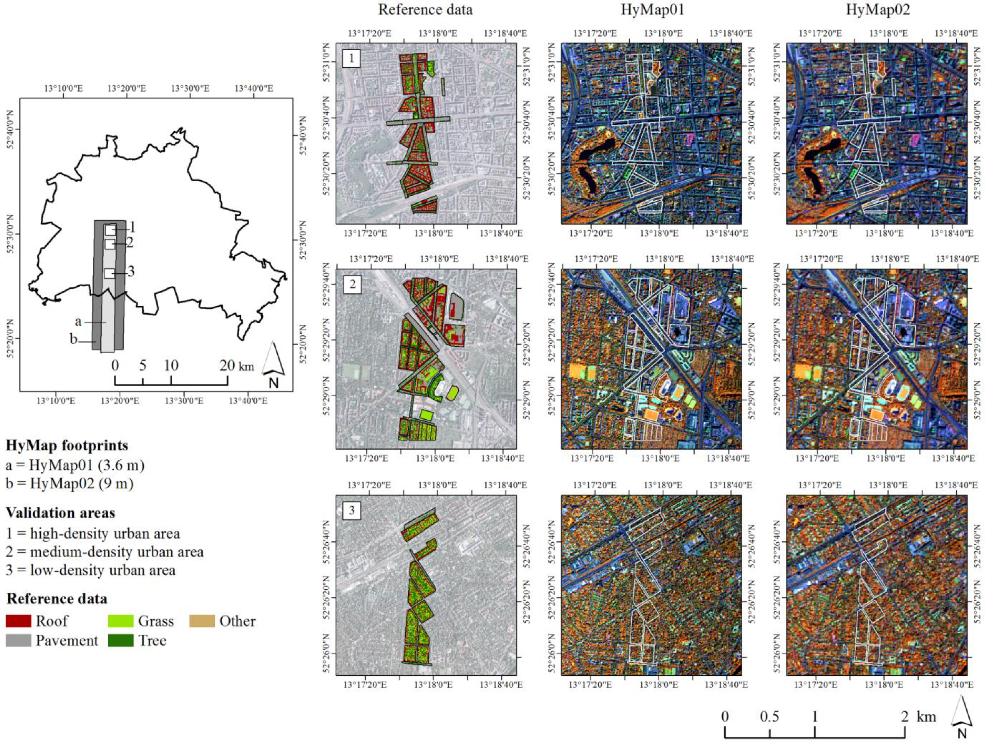
2.1. Study Area

The study region covers a subset of the urban–rural gradient of Berlin, Germany (Figure 1). Along this transect we selected three validation areas of different urban structure types, which include manifold man-made materials and vegetation types typical for the city. The “high-density urban area” represents an inner-city commercial and residential zone with dense building block structures. The “medium-density urban area” includes residential zones with less dense perimeter block or row house structures as well as industrial zones with large, paved areas. The “low-density urban area” represents a suburban residential zone with mainly detached and semi-detached housing patterns with associated private gardens. All three validation areas include green spaces and street corridors of different sizes. Given this makeup, a representative spectrally and spatially challenging heterogeneous urban environment was considered for our experiments.

2.2. Image Data

We used imaging spectrometer data acquired by the HyMap sensor during the HyEurope 2009 Campaign of the German Aerospace Centre (DLR) on 20 August 2009. The aircraft was flown over the study area twice, with identical nadir position but at different altitudes of 2005 and 4750 m. This resulted in two independently acquired scenes with spatial resolutions of 3.6 m (HyMap01) and 9 m (HyMap02) after image ortho-rectification [44] (Figure 1). Pre-processing to reflectance values encompassed system correction [45] and radiometric correction [46]. The number of spectral bands was reduced from 128 to 111 in order to limit the influence of noise during the analysis. Due to the nearly similar acquisition time around solar noon, the high sub-pixel accuracy achieved during ortho-rectification and the identical radiometric and atmospheric pre-processing, consistency between both images was given for a comparative study.

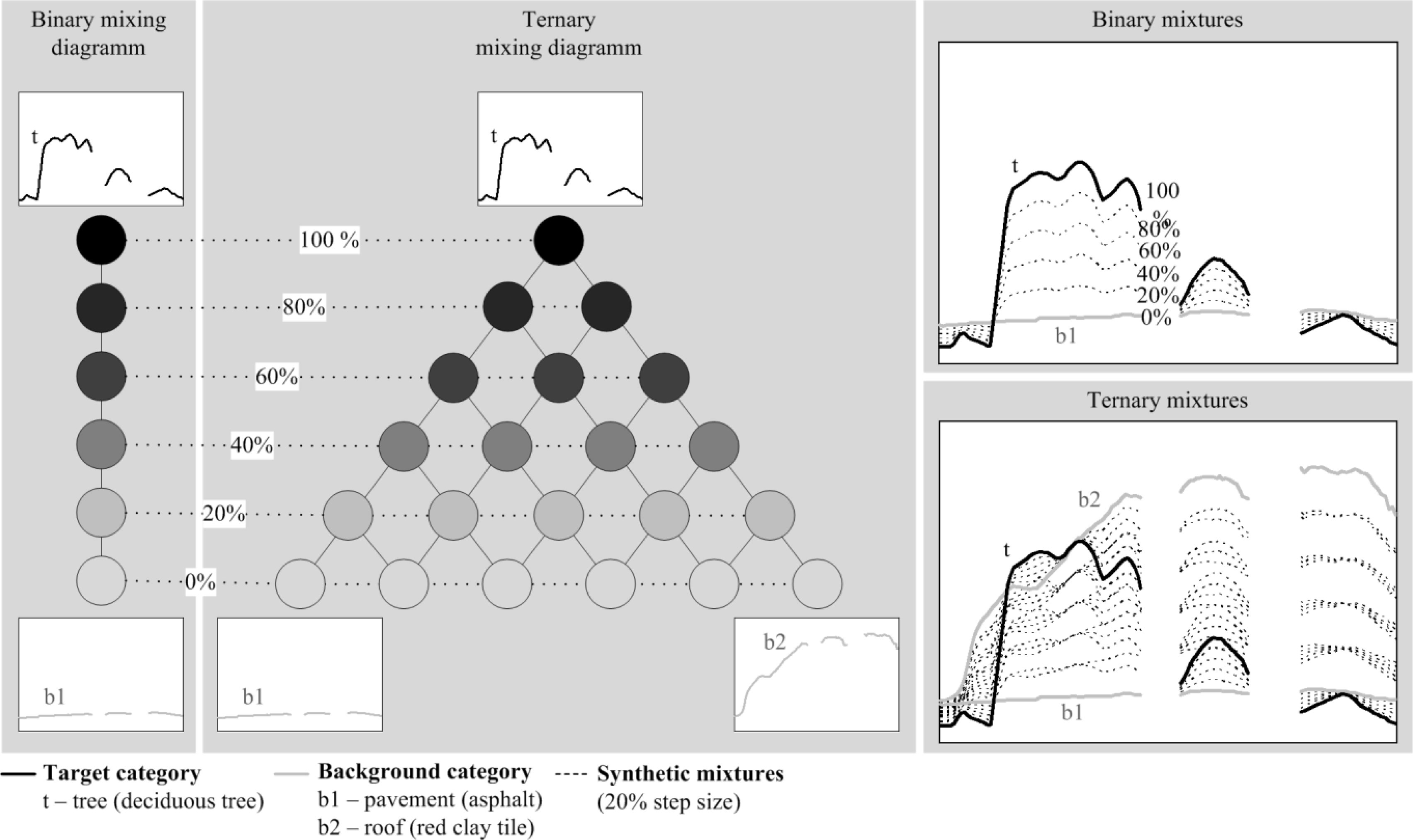
2.3. Spectral Library

We used a library composed of 41 urban material spectra extracted from HyMap01 as database for generating synthetically mixed training data (

Table 1. Categorized image spectral library of urban materials.

Urban Category	Surface Material	No. Spectra
Roof	Red clay tile	4 (a)
	Red cement tile	3 (a)
	Bitumen	5 (b)
	Brown roof tile	1
	Brown roof shingle	1
	White roof material (polyethylene)	1
	White roof material (unknown)	1
	Zinc roof material	1
Pavement	Asphalt	4 (a, b)
	Concrete	2 (b)
Grass	Grass (intensively manicured)	2 (a)
	Grass (extensively manicured)	1
	Grass (dry)	2 (a)
Tree	Deciduous tree	7 (a)
Other	Tartan (sports ground)	1
	Railtrack (concrete sleepers)	1
	Railtrack (wooden sleepers)	1
	Sand (playground)	1
	Soil	1
	Water	1

Multiple spectra per material considered to account for spectral variability due to variations in (a) illumination and shading effects; and (b) material condition.

). Detailed information on the development of the image spectral library was provided in [36], where the library was demonstrated to include relevant spectra necessary for quantifying urban land cover within the same study region. The library includes a representative standard spectrum per material, which was complemented in case of high spectral variability. Complemented spectra account for variations in brightness caused by illumination or shading effects or variations due to differences in material condition. Spectra were categorized into the four urban land cover categories of interest, i.e., roof (17 spectra), pavement (6), grass (5) and tree (7). An additional other (6) category, which did not constitute a category of interest in this work, was used to assign surface types with marginal spatial occurrence (e.g., water, sport grounds covered with artificial turf, etc.).

2.4. Reference Data

We performed a polygon-wise evaluation of results, a common strategy to statistically assess the accuracy of fraction maps derived from urban remote sensing data [10,21]. We used urban blocks from the Berlin Urban Environmental Information System [47] (Figure 1), which constitute a suitable spatial unit for many urban environmental applications [43,48]. Within the three validation areas, block-wise mean fraction values for a total number of 92 urban blocks were calculated from an available high resolution reference land cover map [36]. To guarantee a representative heterogeneous validation data set, we selected 45 building blocks of different urban structure types, 37 street polygons including roads of different sizes, and 10 green spaces consisting of parks, allotment gardens or sport grounds. All urban block polygons were selected within a ±10° off-nadir region to minimize effects of reflectance anisotropy [49] and urban 3D-geometry [4] during validation. This way, spectral effects influenced almost entirely the accuracy of fraction maps.

3. Methods

3.1. Synthetically Mixed Training Data

We followed the concept of synthetically mixed training data for regression modeling [36]. The general idea is to use a spectral library to construct a single quantitative training data set for a given land cover category of interest, a so-called target category. Consisting of pairs of spectra and related mixing fractions, this set is subsequently used as input for regression model training. A fraction map of the target category is derived by applying the model to the image data. The subsequent analysis of several target categories allows for a comprehensive mapping of urban land cover.

While generating synthetically mixed training data, we assume a linear mixing process between materials. It cannot be ruled out that nonlinear mixing effects caused by multiple scattering processes between materials [50,51] may affect mapping results. Yet, quantitative effects of nonlinear mixing on the accuracy of fraction estimates are poorly understood [52]. In the context of urban land cover assessments, linear mixing systematic was frequently adopted and led to valid results [3,5,10,21].

We generated synthetically mixed training data as follows: For each of the four categories of interest, the spectral library was partitioned into (i) a target category (e.g., tree) and (ii) a background category with all remaining categories (e.g., roof, pavement, grass, other). Subsequently, linear mixtures between target and background category spectra were calculated using mixing steps of 20%. This step size was shown to provide sufficient continuous information for quantifying urban land cover using SVR [36]. This resulted in a set of pure spectra, synthetically mixed spectra and related mixing fractions of 0%, 20%, 40%, 60%, 80% and 100% of the respective target category. Spectra within the other category were only used as background. Accordingly, synthetically mixed training data were not derived for the other category and corresponding surface types, such as water or sports grounds covered with artificial turf, were not explicitly mapped.

To account for the mixing complexity, we constructed two different training data sets for each target category (Figure 2). Within the first type of training data (SyMix01), we included all possible binary mixtures between target category spectra and background category spectra. Material combinations within a category were not included. SyMix01 is considered as training data of lower complexity, as only mixtures of two materials were integrated. Within the second type of training data (SyMix02), we included all possible binary mixtures and selected ternary mixtures between target category spectra and background category spectra. In our case, ternary mixtures were calculated as two-fold binary mixtures and included (i) combinations between a target spectrum (mixing fraction of 100%) and a binary mixed background spectrum (mixtures of two background spectra in 20% increments but treated as having a mixing fraction of 0%) or (ii) combinations between a binary mixed target spectrum (mixtures of two target spectra in 20% increments but treated as having a mixing fraction of 100%) and a background spectrum (mixing fraction of 0%). Knowledge on relevant ternary mixtures was derived from visual inspection of digital orthophotos. We considered both combinations between different categories (e.g., “deciduous tree-red clay tile-asphalt” or “deciduous tree-grass-soil”) and combinations within categories (e.g., “deciduous tree-red clay tile-bitumen” or “asphalt-concrete-tree”). This selective approach was study area specific, however, guaranteed the inclusion of higher order mixtures while at the same time prevented an excessive amount of training samples due to the variety of possible combinations. SyMix02 is considered as training data of higher complexity, as mixtures of two and three materials were integrated. The sample sizes of the eight training data sets, which are each used separately to train one regression model per target category and mixing complexity, are reported in

Table 2. Number of training samples per target category used for regression modeling.

Training Data Set	Roof	Pavement	Grass	Tree
SyMix01	1673	881	761	993
SyMix02	3092	1970	1202	1254

.

3.2. Support Vector Regression (SVR)

Emanating from the field of kernel-based machine learning methods, SVR has been established in remote sensing research, mainly as a powerful, nonlinear technique for quantifying biophysical/chemical plant properties [31,33]. Details on the underlying concepts of SVR can be found in [18]. In general, SVR estimates the linear dependency between pairs of n-dimensional input vectors and 1-dimensional target variables by fitting an optimal approximating hyperplane to a set of training samples. The optimal hyperplane is defined by a linear regression model that is found by solving a convex optimization problem. The most common SVR formulation thereby minimizes Vapnik’s ɛ-insensitive cost function. Embedded into a kernel framework, SVR is capable of coping with nonlinear data distributions. By using a kernel function, training samples are mapped into a higher dimensional feature space, which is nonlinearly related to the original space and wherein the new data distribution enables a better fitting of a linear function.

The SVR analysis of this work was carried out with imageSVM [53], which uses the Gaussian kernel function. Parameterization of an SVR required the selection of the kernel parameter σ, the regularization parameter C and the loss function parameter ε. Tuning of the three parameters was carried out via grid search using a cross validation strategy to avoid overfitting.

3.3. Kernel Ridge Regression (KRR)

KRR has been lately introduced for remote sensing applications [32,54]. Detailed information on the theoretical background of KRR can be found in [38]. Similar to SVR, KRR maps the training samples into a higher dimensional feature space by making use of a kernel function. There, KRR minimizes the squared residuals, and can be therefore considered as the kernel version of the regularized least squares regression [32].

The KRR analysis of this work was carried out with the ARTMO software package [54]. KRR modeling required the tuning of two parameters, i.e., the Gaussian kernel function parameter σ and the regularization parameter C. Parameter optimization was carried out via standard cross validation.

3.4. Neural Network Regression (NN)

Artificial neural networks were one of the first non-parametric, nonlinear techniques to be used for remote sensing applications [25,34,35]. Details on the theoretical concepts of NN can be found in [39]. A NN is a model that establishes the relationship between input vectors and output variables through a connected structure of neurons organized in layers. Each neuron basically performs a linear regression followed by a nonlinear function. Neurons of different layers are interconnected with the corresponding links, i.e., weights. NN modeling requires the selection of a NN structure, the initialization of weights, shape of nonlinearity and learning rate as well as the regularization of parameters to avoid overfitting [32].

The NN analysis of this work was carried out with ARTMO [54], which uses a fully connected standard multi-layer perceptron and a hyperbolic tangent as nonlinear activation function. We selected just one hidden layer of neurons, weights were randomly initialized and the NN structure was optimized using a squared loss function. Model parameterization was carried out via a standard cross validation procedure.

3.5. Random Forest Regression (RFR)

Random forest [40], an ensemble method based on multiple decision trees, has been used in a variety of remote sensing studies [30,55]. Decision trees are non-parametric predictive models, which are based on a multistage decision scheme. They exist in the form of classification and regression trees, as they are suited to predict both discrete and continuous output variables. The tree structure consists of a root node, internal nodes (splits) and terminal nodes (leaves). At each split and until a leaf node is reached, a decision rule is applied to partition the training data recursively into increasing number of smaller homogenous subsets. A target variable is assigned to each sample according to the leaf node [56,57]. As an ensemble method, RF combines the results of many individual decision trees in order to improve the overall prediction performance. Independent decision trees are created through bagging (bootstrap aggregation), where each decision tree uses a random sample (with replacement), and through random feature selection at each split node. Training samples that are excluded, so-called “out-of-bag” (OOB) samples, can be used for independent validation. For the regression case, the final prediction is obtained by averaging the results of individual trees [40].

The random forest regression analysis was carried out using imageRF [58]. The number of trees was set to 100, the ratio of bootstrap data to OOB data was 2/3–1/3 and the number of randomly selected features corresponded to the square root of all features. For each tree, the respective OOB data was used for predicting and the accuracy of combined results was assessed using the OBB error. The learning curve of the OOB error with increasing number of trees was used to verify whether reliable parameters were set.

3.6. Partial Least Squares Regression (PLSR)

Partial least squares regression [41] has been widely used for quantifying vegetation properties by means of hyperspectral data [33,59,60]. PLSR is a multivariate method that is very similar to principle component regression, where the dimensionality of the input features is first reduced with respect to their information content followed by multiple linear regression modeling. Unlike principle component regression, where only correlations within the input feature space are considered, PLSR transforms the input features into a few uncorrelated latent vectors, which are generated not only with respect to their variance but also with respect to their explanatory power to predict a response variable during linear regression. Latent vectors are statistically independent linear combinations of the original input features. PLSR is well suited for handling highly correlated data [41,61].

The PLSR analysis of this work was carried out using autopls [60]. Autopls includes an iterative backward selection of latent vectors, which reduces the number of predictors in the regression following [62,63]. A cross-validation strategy was used to prevent overfitting during model training. The final model was selected based on the learning curve during backward selection, i.e., the model with the smallest training error was used for regression modeling on the image.

3.7. Validation

Validation of results was carried out by comparing modeled versus reference fractions at urban block scale (block-wise mean values). We calculated both class-wise accuracy scores (performance measures for a single fraction map of a target category) and average accuracy scores (mean of class-wise accuracies over all categories). We used the mean absolute error (MAE) and the root mean square error (RMSE) as measures of accuracy. MAE and RMSE are defined as

$$\mathit{MAE}=\frac{1}{n}\sum _{i=1}^n\left|y_i-x_i\right|$$

(1)

$$\mathit{RMSE}=\sqrt{\frac{1}{n}\sum _{i=1}^n{\left(y_i-x_i\right)}^2}$$

(2)

where y_i are the modeled fractions, x_i are the reference fractions and n the number of validation samples. To evaluate the goodness of fit between estimated and reference fractions, we used the coefficient of determination (R²), given by

$$R^2=\frac{{\left({\sum }_{i=1}^n(x_i-\overline{x})(y_i-\overline{y})\right)}^2}{{\sum }_{i=1}^n{\left(x_i-\overline{x}\right)}^2{\sum }_{i=1}^n{\left(y_i-\overline{y}\right)}^2}$$

(3)

where ȳ and x̄ are the averages of the modeled and reference fractions, as well as the slope and the intercept of a fitted least squares linear regression model.

4. Experimental Setup and Results

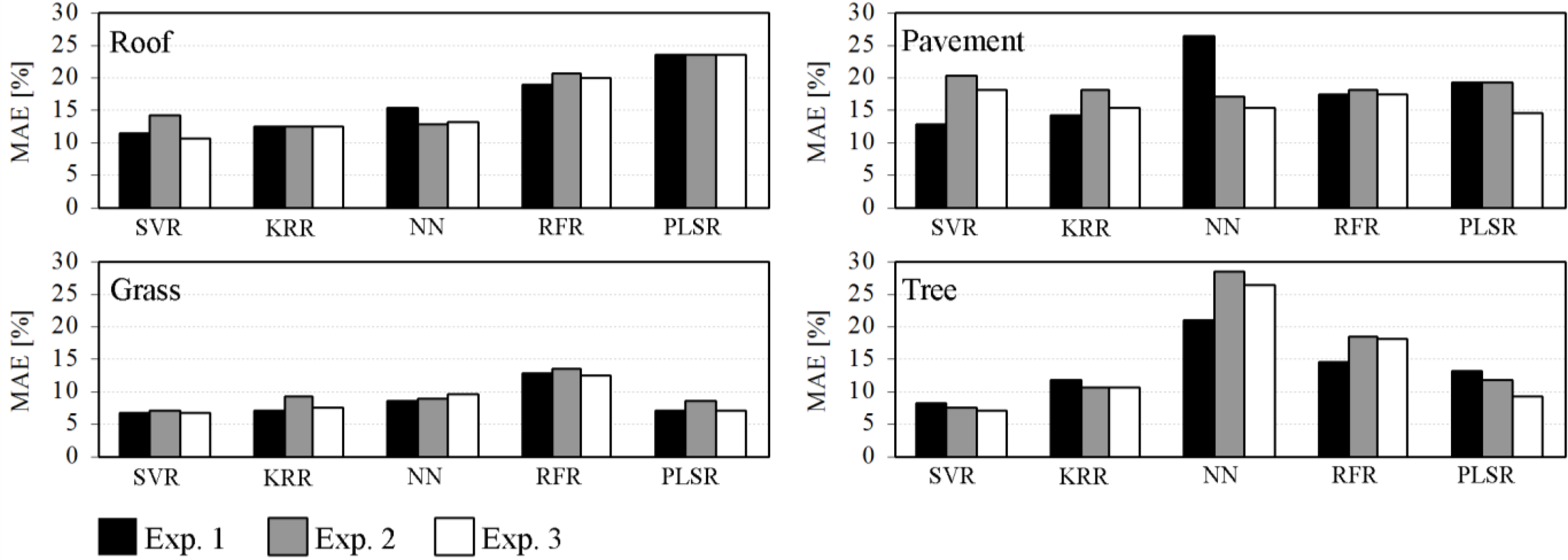
4.1. Experimental Setup

To answer the research questions, we carried out three experiments using the two HyMap images (HyMap01, HyMap02), synthetically mixed training data at different complexities (SyMix01, SyMix02) and five different regression techniques (SVR, KRR, NN, RFR and PLSR). The experiments are summarized as follows:

• Exp. 1: We investigated the efficiency of the regression techniques to utilize synthetically mixed training data for quantifying urban land cover. For each regressor and each target category, we trained one regression model using SyMix01. Subsequently, we applied the models to HyMap01 to derive fraction maps at 3.6 m spatial resolution.
• Exp. 2: We investigated the influence of coarser resolution image data on the quality of model predictions. We therefore applied regression models used in Exp. 1 to HyMap02 to derive fraction maps at 9 m spatial resolution.
• Exp. 3: We investigated whether more complex synthetic mixtures help to improve fraction estimates from the coarser resolution data. For each regressor and each target category, we trained one regression model using SyMix02. Subsequently, we derived a second set of fraction maps at 9 m spatial resolution by applying models to HyMap02.

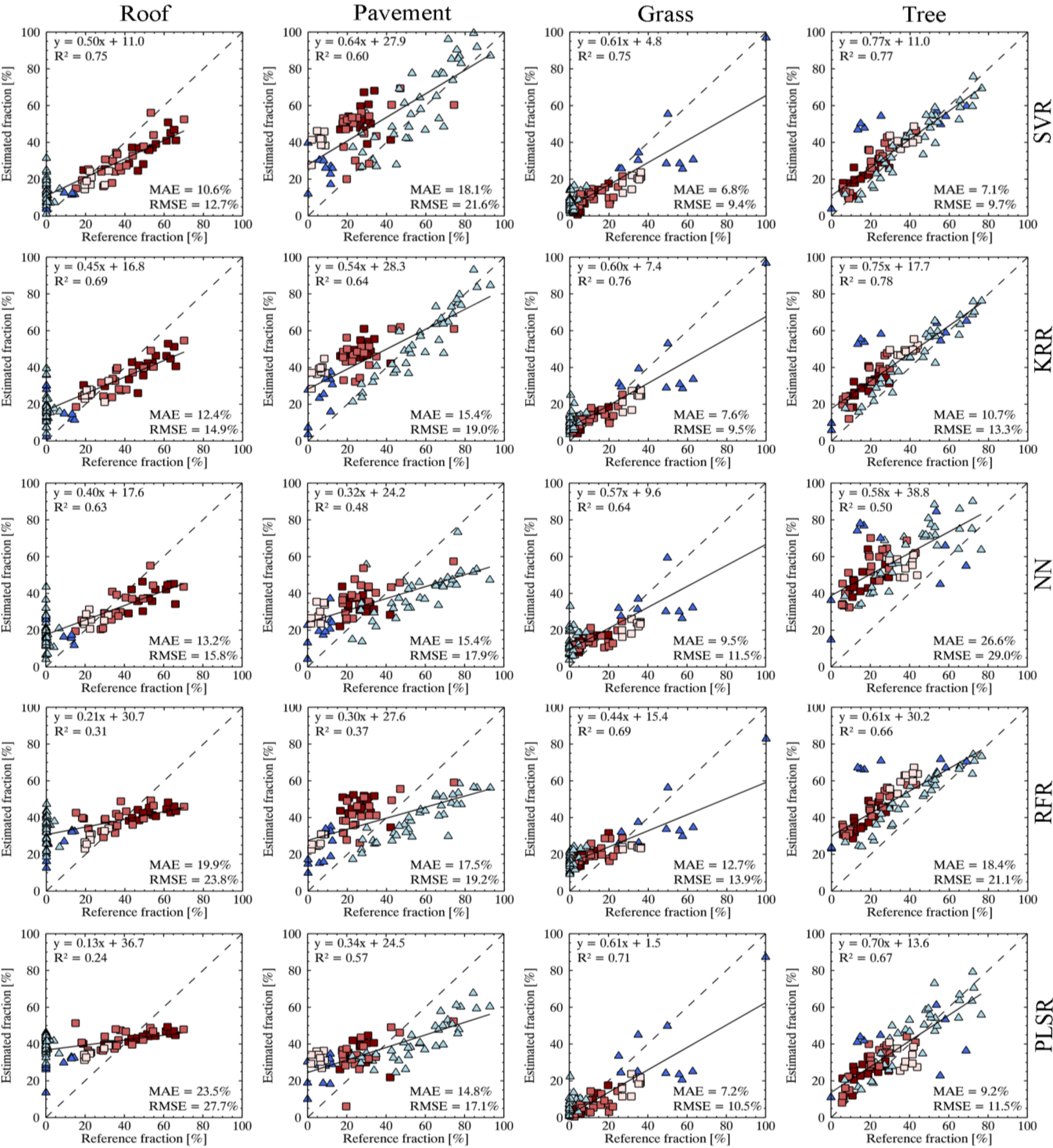
4.2. Average and Class-Wise Accuracies of Experimental Results

Average accuracy scores of urban land cover fraction estimates are reported in

Table 3. Average accuracies of urban land cover fraction maps derived from different regression algorithms for the three experiments. Highest accuracy scores for each experiment are highlighted by bold numbers.

Experiment	Data	Method	MAE (%)	RMSE (%)	R2	Slope	Intercept
Exp. 1	HyMap01 SyMix01	SVR	9.8	12.5	0.76	0.62	12.5
		KRR	11.5	13.8	0.77	0.60	13.8
		NN	17.9	20.8	0.61	0.49	20.8
		RFR	16.0	18.4	0.53	0.35	18.4
		PLSR	15.8	18.8	0.55	0.46	18.8
Exp. 2	HyMap02 SyMix01	SVR	12.3	15.3	0.66	0.56	15.3
		KRR	12.7	15.5	0.70	0.57	15.5
		NN	16.8	19.2	0.54	0.46	19.2
		RFR	17.8	20.4	0.50	0.38	20.4
		PLSR	15.9	18.5	0.51	0.41	18.5
Exp. 3	HyMap02 SyMix02	SVR	10.7	13.4	0.71	0.63	13.4
		KRR	11.5	14.2	0.71	0.59	14.2
		NN	16.2	18.5	0.56	0.47	18.5
		RFR	17.1	19.5	0.51	0.39	19.5
		PLSR	13.7	16.7	0.55	0.45	16.7

. In Exp. 1, both kernel methods SVR and KRR show best performances, with high accuracies (e.g., MAE below 12%, R² above 0.75) at 3.6 m spatial resolution. Results of NN, RFR and PLSR are less accurate. In Exp. 2, deteriorating mapping accuracies are observed for most of the regressors when applying models to the coarser resolution image. Still, both kernel methods SVR and KRR produce considerably high average accuracies (e.g., MAE below 13%, R² above 0.65) while accuracies of NN, RFR and PLSR remain less accurate. NN produces inconsistent results with opposing average accuracy scores, i.e., improving MAE but also decreasing R². In Exp. 3, the increased complexity of the training data particularly improves SVR-, KRR- and PLSR-based estimates. For NN and RFR, only slight improvements are observed. Also, in this experiment, SVR and KRR remain the best performing techniques with high average accuracies (e.g., MAE of 11.5% and below, R² of 0.71).

Class-wise MAE values (Figure 3) reveal the performances of the five regressors when mapping different urban surface types. For a more general evaluation, accuracy scores are classified as highly accurate (MAE below 10%), accurate (MAE between 10% and 15%), sub-optimal (MAE between 15% and 20%) and inaccurate (MAE above 20%). In Exp. 1, both kernel methods SVR and KRR produce accurate roof and pavement, and accurate to highly accurate grass and tree mappings. The performance of NN is highly variable with sub-optimal roof, highly accurate grass and inaccurate pavement and tree estimates. The ability of RFR and PLSR to predict roof and pavement is rather low, with sub-optimal to inaccurate mapping accuracies. In contrast, grass and tree estimates by RFR and PLSR are accurate to highly accurate at 3.6 m spatial resolution.

The impact of the coarser resolution image (Exp. 2) and the training data of higher complexity (Exp. 3) on the quality of fraction maps strongly varies between the regressors and the urban land cover types. Decreasing performances, which are fully compensated for by the more complex training data, are observed for SVR-based roof and KRR-based grass estimates. Both mappings remain accurate to highly accurate at 9 m spatial resolution. Pavement predictions by the kernel methods follow similar trends, however, with only partly compensated accuracies by the more complex training data. This results in degraded, sub-optimal pavement estimates by SVR and KRR on the coarser resolved image. The remaining mappings by SVR and KRR are relatively stable with similar accuracies when compared to results at 3.6 m. NN reveals erratic patterns in accuracy scores between the urban categories, i.e., roof and especially pavement inconsistently improve to accurate and sub-optimal mappings mainly due to the decreased spatial resolution, grass predictions remain stable and highly accurate and the inaccurate tree mapping further deteriorates. The performance of RFR and PLSR for mapping roof at 9 m spatial resolution remains low. Pavement estimates by RFR remain sub-optimal, whereas PLSR predictions improve through integrating training data of higher complexity. The performance of RFR and PLSR to map grass on the coarser resolution image is still high, with relatively stable accuracies between the experiments. Considering the tree category, RFR-based predictions clearly deteriorate at 9 m resulting in sub-optimal performances despite training data of higher complexity. PLSR reveals accurate tree predictions at 9 m, with improved accuracy scores compared to the result on the higher resolved image.

The scatterplots (Figure 4) reveal the regions of agreement and disagreement between reference fractions and modeled urban land cover fractions derived from HyMap02 at 9 m spatial resolution using SyMix02 (Exp. 3). A general representation of how building blocks from different urban densities, street corridors and green spaces influence the accuracies of fraction estimates is given. The accurate roof estimates by SVR, KRR and NN are underlined by the linear data distribution close to the 1:1 diagonal line. Within building blocks, roof fractions are precisely mapped in the low- and medium-density urban area and slightly underestimated within the high-density urban area. One common major source of error for all three regression techniques are misleadingly mapped roof fractions along streets or within green spaces. The lower performance to map pavement by all regressors is explained by a general higher rate of scattering and a characteristic overestimation of fractions within the building blocks of different densities and green spaces. In contrast, pavement fractions mapped along street corridors appear accurate, particularly for KRR. Grass results are accurate for all regressors. Only RFR shows a slight deviation from this trend. The high accuracies of tree estimates by SVR, KRR are underlined by the strong linear correlation with the reference data. PLSR shows similar high performances, however, with increased scattering. The four green spaces, which clearly deviate from the 1:1 diagonal line for both grass and tree estimates, correspond to allotment gardens. These inaccuracies repeatedly occur for all regressors in all experiments and relate to uncertainties in the reference data, as the manual mapping of highly fragmented vegetation patches within allotment gardens appears critical.

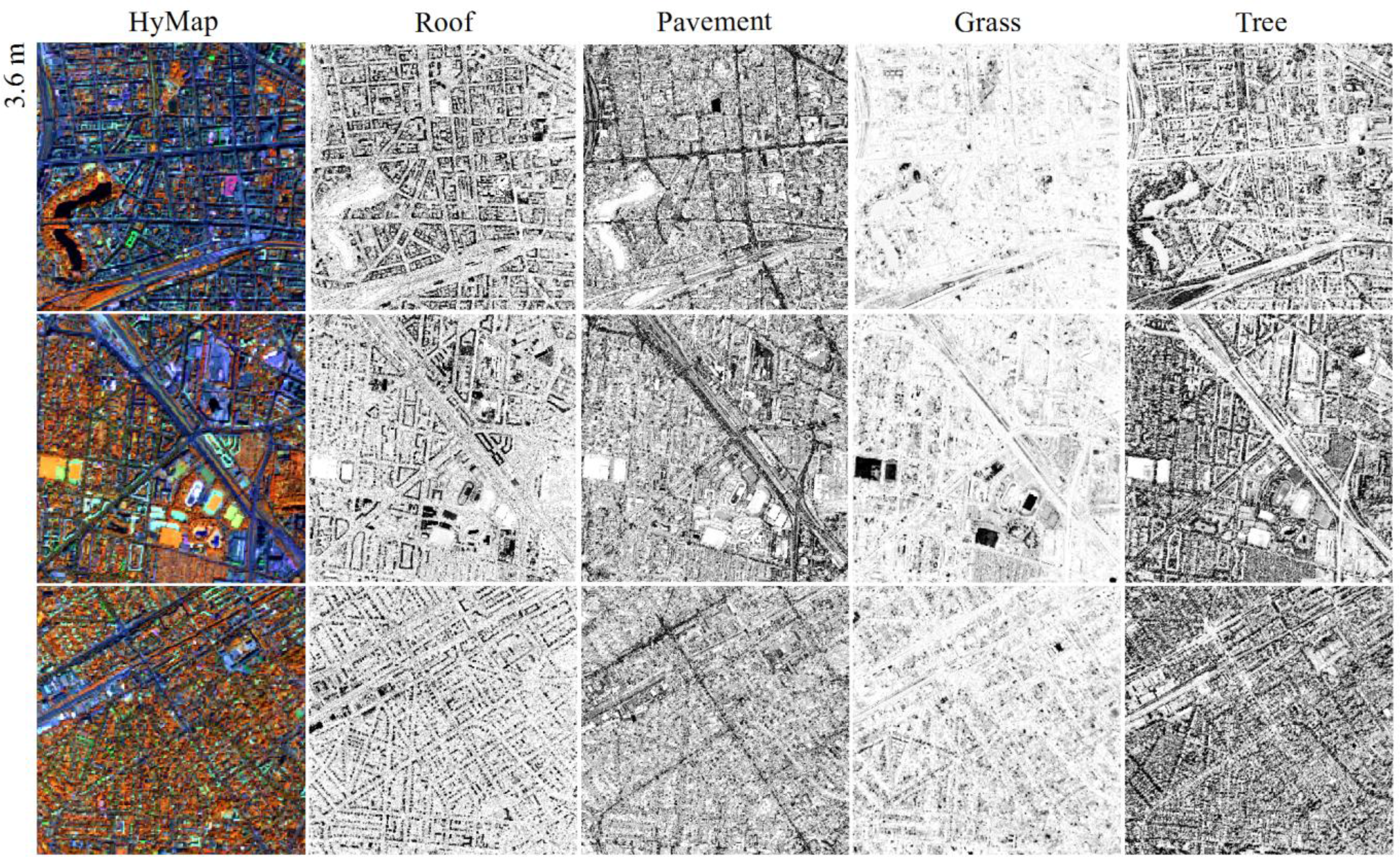
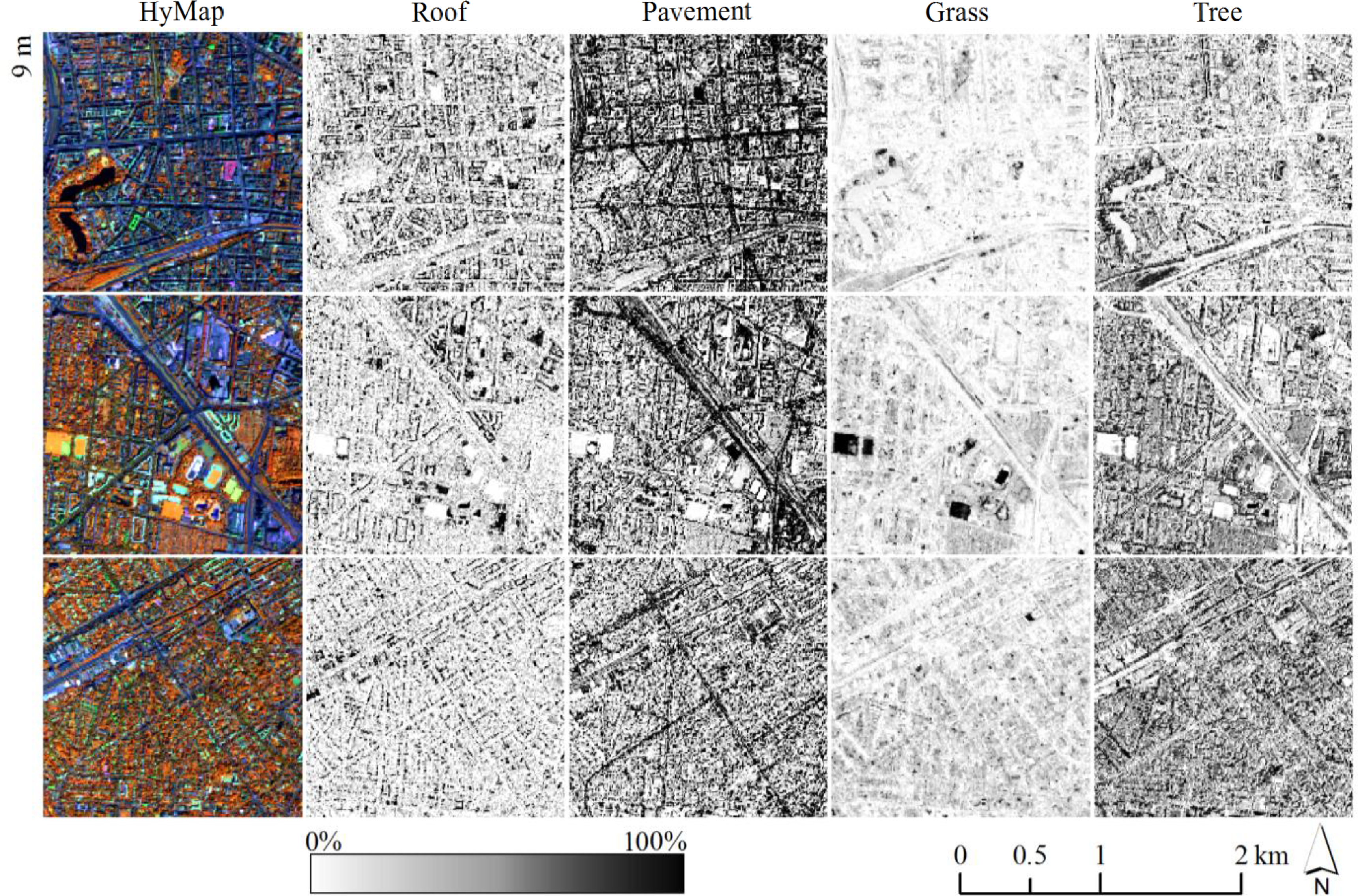
4.3. Quantifying Urban Land Cover at Multiple Spatial Scales Using SVR

Summarizing from the tested regression techniques, SVR and KRR yielded the most accurate land cover estimates at multiple scales. We selected SVR for a pixel-wise representation of urban land cover at 3.6 and 9 m spatial resolution (Figure 5). Results depict the typical structure of Berlin along the urban–rural gradient. The high-density urban area is characterized by a high amount of buildings and paved areas as indicated by the roof and pavement fraction maps. Apart from a few industrial areas and highways, these densities decrease towards the urban fringe. Yet, reported overestimates in pavement fractions within the medium- and low-density urban area are obvious particularly where vegetation, and thus shadowing within vegetation stands, dominate the scenery. High vegetation proportions even within the city center relate to the high amount of green spaces and street trees that characterize the cityscape of Berlin. Nevertheless, a gradual increase in grass and tree fractions is observed when moving towards the urban fringe. Other surface types, such as water bodies in the high-density urban area or sports grounds covered with artificial turf in the medium-density urban area, were only used as background category during processing and appear bright (fractions of 0%) in the maps. Overall, consistent and similar spatial patterns in fraction values are observed between the urban land cover maps at 3.6 and 9 m spatial resolution.

5. Discussion

We tested the combination of five advanced regression techniques with synthetically mixed training data of different complexities for quantifying urban land cover from HyMap data at 3.6 and 9 m spatial resolution. The use of synthetic spectral mixtures poses a straightforward strategy enabling sub-pixel mapping assessments by means of regression analysis. The approach requires a library with relevant material spectra for the study area. Linking the image spectral library to both images was unproblematic due to the consistency between the data sets. Universal spectral databases may be used alternatively, provided that library spectra and imagery are accurately cross-calibrated. The identical inputs from a spectral library used during model training guaranteed a fair methodological comparison. Block-wise accuracy assessment with an independent reference map gave an important insight into the generalization capabilities of the regressors when applied to a real data scenario.

We considered the four thematically meaningful and spectrally challenging urban land cover types roof, pavement, grass and tree. The roof category is a typical example for a spectrally complex class, which is characterized by a multi-modal spectral distribution due to the high number of different materials at different physical conditions and compositions [1,2]. The pavement category is a typical example for a class that is highly subject to spectral similarities. This is due to a low number of spectrally distinct materials, most of them with very similar spectral signatures when compared to dark spectra from background cover types (e.g., street asphalt vs. bituminous roofing materials) [1,2]. Likewise, high spectral similarity between vegetation types impedes the differentiation of grass and tree in such a heterogeneous setup. The spectral complexity of urban materials is further amplified by illumination and shadowing effects. Particularly shaded areas have been reported to influence the accuracy of urban land cover maps derived from hyperspectral imagery [4,6,36]. By choosing the four urban categories, the ability of the tested regression methods to deal with spectral complexity, similarity and variability was explored.

Two major findings can be drawn from Exp. 1, where HyMap data at 3.6 m spatial resolution was used to quantify urban land cover. First, we could once more demonstrate that the concept of synthetically mixed training data enables the use of empirical regression techniques for sub-pixel mapping of single urban land cover categories. Second, we could demonstrate that the quality of fraction maps strongly depends on the selected regression method. Both kernel-based regression techniques SVR and KRR proved to be well suited for quantitatively analyzing impervious and natural urban sub-categories using hyperspectral data. High average accuracies (Table 3) point to the ability of SVR and KRR for a comprehensive quantification of urban land cover. Class-wise accuracies (Figure 3) indicate the efficiency of SVR and KRR to discriminate the challenging urban categories roof, pavement, grass and tree with a low degree of confusion caused by spectral complexity and similarity.

In Exp. 1, SVR and KRR outperformed NN, RFR and PLSR in most cases. They revealed either erratic (NN) or limited (RFR and PLSR) performances, which makes a general evaluation on their use for comprehensively mapping urban land cover from the 3.6 m HyMap data difficult. Yet, all three methods illustrate potential for mapping individual urban categories, e.g., roof and grass by NN and grass and tree by KRR and PLSR, respectively.

The change in spatial resolution from 3.6 m to 9 m implies a loss of spatial detail and, even more important, a significant increase in the number of mixed pixels and in the abundance of different materials contributing to the mixed signal. Overall, both kernel methods SVR and KRR yielded most accurate results on the coarser resolution image. Regression models proved to be stable with regard to the spatial and spectral differences between the two images (Exp. 2) and effectively utilized the additional information provided by more complex ternary mixtures to compensate losses in mapping quality (Exp. 3). The integration of ternary mixtures in addition to the binary mixtures always appears worthwhile, as no negative impacts were observed. These findings are supported by the average accuracy scores (Table 3), which only slightly degrade between Exp. 2 and Exp. 1 (ΔMAE = −2.5% for SVR, ΔMAE = −1.2% for KRR) and clearly improve when comparing Exp. 3 to Exp. 1 (ΔMAE = −0.9% for SVR and 0.0% for KRR). Roof, grass and tree can be mapped at similar high precision by SVR and KRR at 9 m when compared to results at 3.6 m spatial resolution (Figure 3). However, the precise differentiation of pavement from coarser resolution data is challenging. Degraded sub-optimal pavement accuracies obtained by both kernel methods likely relate to the dominance of spectrally similar materials, which become increasingly indistinct and difficult to differentiate at 9 m.

Also in Exp. 2 and 3, SVR and KRR mostly showed superior mapping performances over NN, RFR and PLSR. The suitability of NN to reliably cope with the coarser resolution HyMap data when mapping individual urban land cover categories is ambiguous. For example, roof and particularly pavement estimates are improved to make comparable accuracies to those obtained by both kernel methods. However, this finding is controversial as the enhancement is rather related to the increased pixel size than to the integration of more complex training signatures. Lower performances by RFR and PLSR to map roof and pavement on the coarser resolution data question the use of both methods when mapping the spectrally complex or similar impervious sub-categories, while both methods appear suitable for mapping urban vegetation types.

Results of this comparative study demonstrate that SVR and KRR yielded the most accurate and reliable estimates from HyMap data at 3.6 and 9 m spatial resolution, whereas NN, RFR and PLSR revealed some major limitations. The quality of fraction maps (Figure 5) to depict the typical structure along Berlin’s urban-rural gradient underscores the suitability of SVR to be used along with synthetically mixed training data for quantifying urban land cover at multiple spatial scales. Nevertheless, several aspects appear worthwhile for discussion. First, our regression techniques were regularly adopted in the remote sensing context [32,36,54,60], however, caution must be exercised that different implementations of these algorithms exist. Second, the strategy to consider only selected ternary mixtures using expert knowledge prevented an excessive amount of training samples. Higher order mixtures within the image data that were not accounted for during training may affect the quality of mappings. Yet, achieved accuracies are valid and the efficiency of the regressors to utilize more complex training mixtures was well explored. Third, results demonstrate that even both the best performing kernel methods did not completely overcome well known problems arising from spectral similarities or shadowing. Particularly, the unambiguous quantification of rooftops or paved-areas was not completely possible and uncertainties in fraction maps remain. Typical examples are misleadingly mapped roof fractions along streets or within green spaces and overestimated pavement fractions within most building blocks and green spaces (Figure 4), caused by the spectral similarity between dark roofing materials, street asphalt and canopy shade. The use of multi-sensor approaches that take advantage of information beyond the spectral domain may help to overcome such deficiencies [48]. Here, we fully focused on the opportunities and limitations of hyperspectral information for assessing urban land cover.

6. Conclusions

Exploring the applicability of powerful quantitative methods is crucial for the development of robust, universal modeling approaches that are needed once imaging spectrometer data from spaceborne hyperspectral sensors will be available. In this paper, we investigated the potential of five advanced regression approaches combined with synthetically mixed training data for quantifying urban land cover using HyMap data at 3.6 and 9 m acquired over Berlin, Germany. The universality of the approach for urban sub-pixel mapping was tested by exploring (1) the efficiency of the different regressors to utilize synthetically mixed training data for producing accurate urban land cover maps; (2) the impact of coarser resolution data on the quality of model predictions; and (3) the need to adapt the training data to the mixing complexity of the image. In most cases, both kernel-based approaches SVR and KRR showed superior average and class-wise mapping performances when compared to NN, RFR and PLSR. Average MAE values show that (1) SVR and KRR outperform the remaining regressors by at least 4.3% at 3.6 m spatial resolution; that (2) for SVR and KRR average MAE values increase by 2.5% and 1.2%, respectively, when decreasing the spatial resolution from 3.6 m to 9 m; and that (3) the use of more complex models improves average MAE values by 1.6% and 1.2% for SVR and KRR.

Based on the findings of this case study, we conclude that the use of synthetically mixed training data is well suited for quantifying spectrally challenging urban land cover types by means of empirical regression modeling. The problems in setting up such approaches as mentioned in the introduction are therefore overcome. At the same time, the general strength of kernel regression methods for urban land cover assessments is illustrated, which had been extensively demonstrated for per-pixel classification problems. Such regression approaches can, hence, be incorporated into quantitative mapping. SVR and KRR models proved to be stable with regard to the amplified mixing scenario and well utilized the added value of more complex training mixtures to cope with deficiencies of coarser resolution data. However, urban land cover assessments on a purely spectral basis will always bear limitations and specific challenges such as spectral similarities between land cover types or confusion caused by shadowing will always remain.

The combination of advanced regression techniques with synthetically mixed training data is straightforward, repeatable and relies on the availability of a spectral library relevant for the study area. Compared to per-pixel classifiers, the proposed workflow relativizes the mixed pixel problem typical for urban remote sensing data. This is important for future studies, where the reliability, validity and general transferability of the approach on image data from different sensor types and different urban areas will be tested.

References

1. Heiden, U.; Segl, K.; Roessner, S.; Kaufmann, H. Determination of robust spectral features for identification of urban surface materials in hyperspectral remote sensing data. Remote Sens. Environ 2007, 111, 537–552. [Google Scholar]
2. Herold, M.; Roberts, D.A.; Gardner, M.E.; Dennison, P.E. Spectrometry for urban area remote sensing—Development and analysis of a spectral library from 350 to 2400 nm. Remote Sens. Environ 2004, 91, 304–319. [Google Scholar]
3. Small, C. High spatial resolution spectral mixture analysis of urban reflectance. Remote Sens. Environ 2003, 88, 170–186. [Google Scholar]
4. Van der Linden, S.; Hostert, P. The influence of urban structures on impervious surface maps from airborne hyperspectral data. Remote Sens. Environ 2009, 113, 2298–2305. [Google Scholar]
5. Franke, J.; Roberts, D.A.; Halligan, K.; Menz, G. Hierarchical multiple endmember spectral mixture analysis (MESMA) of hyperspectral imagery for urban environments. Remote Sens. Environ 2009, 113, 1712–1723. [Google Scholar]
6. Roessner, S.; Segl, K.; Heiden, U.; Kaufmann, H. Automated differentiation of urban surfaces based on airborne hyperspectral imagery. IEEE Trans. Geosci. Remote Sens 2001, 39, 1525–1532. [Google Scholar]
7. Herold, M.; Gardner, M.E.; Roberts, D.A. Spectral resolution requirements for mapping urban areas. IEEE Trans. Geosci. Remote Sens 2003, 41, 1907–1919. [Google Scholar]
8. Gamba, P.; Dell’Acqua, F. Spectral resolution in the context of very high resolution urban remote sensing. In Urban Remote Sensing; Quattrochi, D.W., Ed.; CRC Press Inc: New York, NY, USA, 2006; pp. 377–391. [Google Scholar]
9. Van der Linden, S.; Janz, A.; Waske, B.; Eiden, M.; Hostert, P. Classifying segmented hyperspectral data from a heterogeneous urban environment using support vector machines. J. Appl. Remote Sens 2007, 1, 013543. [Google Scholar]
10. Powell, R.L.; Roberts, D.A.; Dennison, P.E.; Hess, L.L. Sub-pixel mapping of urban land cover using multiple endmember spectral mixture analysis: Manaus, Brazil. Remote Sens. Environ 2007, 106, 253–267. [Google Scholar]
11. Camps-Valls, G.; Bruzzone, L. Kernel-based methods for hyperspectral image classification. IEEE Trans. Geosci. Remote Sens 2005, 43, 1351–1362. [Google Scholar]
12. Melgani, F.; Bruzzone, L. Classification of hyperspectral remote sensing images with support vector machines. IEEE Trans. Geosci. Remote Sens 2004, 42, 1778–1790. [Google Scholar]
13. Pal, M.; Mather, P.M. Some issues in the classification of DAIS hyperspectral data. Int. J. Remote Sens 2006, 27, 2895–2916. [Google Scholar]
14. Colgan, M.S.; Baldeck, C.A.; Feret, J.-B.; Asner, G.P. Mapping savanna tree species at ecosystem scales using support vector machine classification and BRDF correction on airborne hyperspectral and LiDAR data. Remote Sens 2012, 4, 3462–3480. [Google Scholar]
15. Im, J.; Jensen, J.R.; Jensen, R.R.; Gladden, J.; Waugh, J.; Serrato, M. Vegetation cover analysis of hazardous waste sites in Utah and Arizona using hyperspectral remote sensing. Remote Sens 2012, 4, 327–353. [Google Scholar]
16. Clark, M.L.; Roberts, D.A. Species-level differences in hyperspectral metrics among tropical rainforest trees as determined by a tree-based classifier. Remote Sens 2012, 4, 1820–1855. [Google Scholar]
17. Camps-Valls, G.; Bruzzone, L. (Eds.) Kernel Methods for Remote Sensing Data Analysis; John Wiley & Sons, Inc: New York, NY, USA, 2009.
18. Schölkopf, B.; Smola, A.J. Learning with Kernels-Support Vector Machines, Regularization, Optimization, and Beyond; MIT Press: Cambridge, MA, USA, 2002. [Google Scholar]
19. Tuia, D.; Camps-Valls, G. Urban image classification with semisupervised multiscale cluster kernels. IEEE J. Sel. Top. Appl. Earth Observ. Remote Sens 2011, 4, 65–74. [Google Scholar]
20. Roberts, D.A.; Gardner, M.; Church, R.; Ustin, S.; Scheer, G.; Green, R.O. Mapping chaparral in the Santa Monica Mountains using multiple endmember spectral mixture models. Remote Sens. Environ 1998, 65, 267–279. [Google Scholar]
21. Roberts, D.A.; Quattrochi, D.A.; Hulley, G.C.; Hook, S.J.; Green, R.O. Synergies between VSWIR and TIR data for the urban environment: An evaluation of the potential for the hyperspectral infrared imager (HyspIRI) decadal survey mission. Remote Sens. Environ 2012, 117, 83–101. [Google Scholar]
22. Bauer, M.E.; Loffelholz, B.C.; Wilson, B. Estimating and mapping impervious surface area by regression analysis of Landsat imagery. In Remote Sensing of Impervious Surfaces; Weng, Q., Ed.; CRC Press: London, UK, 2008; pp. 3–19. [Google Scholar]
23. Van de Voorde, T.; Jacquet, W.; Canters, F. Mapping form and function in urban areas: An approach based on urban metrics and continuous impervious surface data. Landsc. Urban Plann 2011, 102, 143–155. [Google Scholar]
24. Pu, R.; Gong, P.; Michishita, R.; Sasagawa, T. Spectral mixture analysis for mapping abundance of urban surface components from the Terra/ASTER data. Remote Sens. Environ 2008, 112, 939–954. [Google Scholar]
25. Van de Voorde, T.; de Roeck, T.; Canters, F. A comparison of two spectral mixture modelling approaches for impervious surface mapping in urban areas. Int. J. Remote Sens 2009, 30, 4785–4806. [Google Scholar]
26. Im, J.; Lu, Z.; Rhee, J.; Quackenbush, L.J. Impervious surface quantification using a synthesis of artificial immune networks and decision/regression trees from multi-sensor data. Remote Sens. Environ 2012, 117, 102–113. [Google Scholar]
27. Yuan, F.; Wu, C.; Bauer, M.E. Comparison of spectral analysis techniques for impervious surface estimation using Landsat imagery. Photogramm. Eng. Remote Sens 2008, 74, 1045–1055. [Google Scholar]
28. Yang, L.M.; Xian, G.; Klaver, J.M.; Deal, B. Urban land-cover change detection through sub-pixel imperviousness mapping using remotely sensed data. Photogramm. Eng. Remote Sens 2003, 69, 1003–1010. [Google Scholar]
29. Esch, T.; Himmler, V.; Schorcht, G.; Thiel, M.; Wehrmann, T.; Bachofer, F.; Conrad, C.; Schmidt, M.; Dech, S. Large-area assessment of impervious surface based on integrated analysis of single-date Landsat-7 images and geospatial vector data. Remote Sens. Environ 2009, 113, 1678–1690. [Google Scholar]
30. Walton, J.T. Subpixel urban land cover estimation: Comparing cubist, random forests, and support vector regression. Photogramm. Eng. Remote Sens 2008, 74, 1213–1222. [Google Scholar]
31. Camps-Valls, G.; Bruzzone, L.; Rojo-Alvarez, J.L.; Melgani, F. Robust support vector regression for biophysical variable estimation from remotely sensed images. IEEE Geosci. Remote Sens. Lett 2006, 3, 339–343. [Google Scholar]
32. Verrelst, J.; Munoz, J.; Alonso, L.; Delegido, J.; Pablo Rivera, J.; Camps-Valls, G.; Moreno, J. Machine learning regression algorithms for biophysical parameter retrieval: Opportunities for Sentinel-2 and -3. Remote Sens. Environ 2012, 118, 127–139. [Google Scholar]
33. Yu, K.; Leufen, G.; Hunsche, M.; Noga, G.; Chen, X.; Bareth, G. Investigation of leaf diseases and estimation of chlorophyll concentration in seven barley varieties using fluorescence and hyperspectral indices. Remote Sens 2013, 6, 64–86. [Google Scholar]
34. Bacour, C.; Baret, F.; Beal, D.; Weiss, M.; Pavageau, K. Neural network estimation of LAI, fAPAR, fCover and LAIxC(ab), from top of canopy MERIS reflectance data: Principles and validation. Remote Sens. Environ 2006, 105, 313–325. [Google Scholar]
35. Cernicharo, J.; Verger, A.; Camacho, F. Empirical and physical estimation of canopy water content from CHRIS/PROBA data. Remote Sens 2013, 5, 5265–5284. [Google Scholar]
36. Okujeni, A.; van der Linden, S.; Tits, L.; Somers, B.; Hostert, P. Support vector regression and synthetically mixed training data for quantifying urban land cover. Remote Sens. Environ 2013, 137, 184–197. [Google Scholar]
37. Stuffler, T.; Förster, K.; Hofer, S.; Leipold, M.; Sang, B.; Kaufmann, H.; Penné, B.; Mueller, A.; Chlebek, C. Hyperspectral imaging—An advanced instrument concept for the EnMAP mission (Environmental Mapping and Analysis Programme). Acta Astronaut 2009, 65, 1107–1112. [Google Scholar]
38. Hastie, T.; Tibshirani, R.; Friedman, J. The Elements of Statistical Learning-Data Mining, Inference, and Prediction, 2nd ed.; Springer: New York, NY, USA, 2009. [Google Scholar]
39. Haykin, S. Neural Networks—A Comprehensive Foundation, 2nd ed.; Prentice Hall: New York, NY, USA, 1999. [Google Scholar]
40. Breiman, L. Random forests. Mach. Learn 2001, 45, 5–32. [Google Scholar]
41. Wold, S.; Sjostrom, M.; Eriksson, L. PLS-regression: A basic tool of chemometrics. Chemometr. Intell. Lab. Syst 2001, 58, 109–130. [Google Scholar]
42. Cadenasso, M.L.; Pickett, S.T.A.; Schwarz, K. Spatial heterogeneity in urban ecosystems: Reconceptualizing land cover and a framework for classification. Front. Ecol. Environ 2007, 5, 80–88. [Google Scholar]
43. Pauleit, S.; Duhme, F. Assessing the environmental performance of land cover types for urban planning. Landsc. Urban Plann 2000, 52, 1–20. [Google Scholar]
44. Schläpfer, D.; Richter, R. Geo-atmospheric processing of airborne imaging spectrometry data. Part 1: Parametric orthorectification. Int. J. Remote Sens 2002, 23, 2609–2630. [Google Scholar]
45. Cocks, T.; Jenssen, R.; Stewart, A.; Wilson, I.; Shields, T. The HyMap™ airborne hyperspectral sensor: The system, calibration and performance. Proceedings of the 1’st EARSeL Workshop on Imaging Spectroscopy, Zurich, Switzerland, 6–8 October 1998; pp. 37–42.
46. Richter, R.; Schläpfer, D. Geo-atmospheric processing of airborne imaging spectrometry data. Part 2: Atmospheric/topographic correction. Int. J. Remote Sens 2002, 23, 2631–2649. [Google Scholar]
47. SenStadt, Berlin Urban and Environmental Information System (UEIS). Available online: http://www.stadtentwicklung.berlin.de/umwelt/umweltatlas (accessed on 4 July 2014).
48. Heiden, U.; Heldens, W.; Roessner, S.; Segl, K.; Esch, T.; Mueller, A. Urban structure type characterization using hyperspectral remote sensing and height information. Landsc. Urban Plann 2012, 105, 361–375. [Google Scholar]
49. Schiefer, S.; Hostert, P.; Damm, A. Correcting brightness gradients in hyperspectral data from urban areas. Remote Sens. Environ 2006, 101, 25–37. [Google Scholar]
50. Borel, C.C.; Gerstl, S.A.W. Nonlinear spectral mixing models for vegetative and soil surfaces. Remote Sens. Environ 1994, 47, 403–416. [Google Scholar]
51. Roberts, D.A.; Smith, M.O.; Adams, J.B. Green vegetation, nonphotosynthetic vegetation, and soils in AVIRIS data. Remote Sens. Environ 1993, 44, 255–269. [Google Scholar]
52. Somers, B.; Asner, G.P.; Tits, L.; Coppin, P. Endmember variability in spectral mixture analysis: A review. Remote Sens. Environ 2011, 115, 1603–1616. [Google Scholar]
53. Rabe, A.; van der Linden, S.; Hostert, P. ImageSVM, Version 2.1. Available online: http://www.imagesvm.net/ (accessed on 4 July 2014).
54. Rivera Caicedo, J.P.; Verrelst, J.; Munoz-Mari, J.; Moreno, J.; Camps-Valls, G. Toward a semiautomatic machine learning retrieval of biophysical parameters. IEEE J. Sel. Top. Appl. Earth Observ. Remote Sens 2014, 7, 1249–1259. [Google Scholar]
55. Chan, J.C.-W.; Paelinckx, D. Evaluation of random forest and adaboost tree-based ensemble classification and spectral band selection for ecotope mapping using airborne hyperspectral imagery. Remote Sens. Environ 2008, 112, 2999–3011. [Google Scholar]
56. Friedl, M.A.; Brodley, C.E. Decision tree classification of land cover from remotely sensed data. Remote Sens. Environ 1997, 61, 399–409. [Google Scholar]
57. Breiman, L.; Friedman, J.H.; Olshen, R.A.; Stone, C.J. Classification and Regression Trees; Wadsworth & Brooks/Cole Advanced Books & Software: Monterey, CA, USA, 1984. [Google Scholar]
58. Waske, B.; van der Linden, S.; Oldenburg, C.; Jakimow, B.; Rabe, A.; Hostert, P. ImageRF—A user-oriented implementation for remote sensing image analysis with random forests. Environ. Modell. Softw 2012, 35, 192–193. [Google Scholar]
59. Smith, M.L.; Martin, M.E.; Plourde, L.; Ollinger, S.V. Analysis of hyperspectral data for estimation of temperate forest canopy nitrogen concentration: Comparison between an airborne (AVIRIS) and a spaceborne (Hyperion) sensor. IEEE Trans. Geosci. Remote Sens 2003, 41, 1332–1337. [Google Scholar]
60. Schmidtlein, S.; Feilhauer, H.; Bruelheide, H. Mapping plant strategy types using remote sensing. J. Veg. Sci 2012, 23, 395–405. [Google Scholar]
61. Feilhauer, H.; Asner, G.P.; Martin, R.E.; Schmidtlein, S. Brightness-normalized partial least squares regression for hyperspectral data. J. Quant. Spectrosc. Radiat. Transf 2010, 111, 1947–1957. [Google Scholar]
62. Chong, I.-G.; Jun, C.-H. Performance of some variable selection methods when multicollinearity is present. Chemometr. Intell. Lab. Syst 2005, 78, 103–112. [Google Scholar]
63. Westad, F.; Martens, H. Variable selection in near infrared spectroscopy based on significance testing in partial least squares regression. J. Near Infrared Spectrosc 2000, 8, 117–124. [Google Scholar]
Figure 1. Study region along Berlin’s urban-rural gradient. The high resolution reference data and the HyMap images (R = 833 nm, G = 1652 nm, B = 632 nm) for the three validation areas are illustrated (polygons indicate the urban blocks used for validation).
Remotesensing 06 06324f1
Figure 2. Generation of binary and ternary synthetic mixtures.
Remotesensing 06 06324f2
Figure 3. Class-wise mean absolute error (MAE) of urban land cover fraction maps derived from different regression algorithms for the three experiments.
Remotesensing 06 06324f3
Figure 4. Scatterplots of roof, pavement, grass and tree estimates compared to reference data at urban block scale. Results of Exp. 3 (HyMap02, SyMix02) are presented. The following symbols are used: Squares = building blocks (dark red = high-density-, red = medium-density-, light red = low-density urban area); triangles = green spaces (blue), street polygons (light blue).
Remotesensing 06 06324f4
Figure 5. SVR-based fraction maps of roof, pavement, grass and tree at 3.6 m (Exp. 1) and 9 m (Exp. 3) spatial resolution. Fraction maps were linearly stretched between 0% and 100%. For information on the locations of the individual subsets, the reader is referred to Figure 1.
Remotesensing 06 06324f5aRemotesensing 06 06324f5b