Algorithm for Extracting Digital Terrain Models under Forest Canopy from Airborne LiDAR Data

Abstract

Extracting digital elevation models (DTMs) from LiDAR data under forest canopy is a challenging task. This is because the forest canopy tends to block a portion of the LiDAR pulses from reaching the ground, hence introducing gaps in the data. This paper presents an algorithm for DTM extraction from LiDAR data under forest canopy. The algorithm copes with the challenge of low data density by generating a series of coarse DTMs by using the few ground points available and using trend surfaces to interpolate missing elevation values in the vicinity of the available points. This process generates a cloud of ground points from which the final DTM is generated. The algorithm has been compared to two other algorithms proposed in the literature in three different test sites with varying degrees of difficulty. Results show that the algorithm presented in this paper is more tolerant to low data density compared to the other two algorithms. The results further show that with decreasing point density, the differences between the three algorithms dramatically increased from about 0.5m to over 10m.

1. Introduction

Airborne light detection and ranging (LiDAR) is an active remote sensing technology that uses aircraft-mounted laser scanning systems in conjunction with a positioning and orientation system (POS) for ranging purposes [1]. The system measures the distance between the laser scanner and reflected objects on the ground (or the ground itself) by considering the round-trip time taken by a laser pulse to travel from the sensor to the reflecting surface and back.

The use of airborne LiDAR technology (hereafter, simply referred to as LiDAR) in forestry applications has been increasing constantly in the past decade. This increasing trend in the use of LiDAR technology in forestry applications can be attributed to both promising results obtained in applications of LiDAR technology to forestry (e.g., [2–7]) and the maturity of the LiDAR technology over time; for example, increased pulse rates and the introduction of full-waveform LiDAR [8]. Unlike conventional LiDAR sensors, which can record up to four returns from multiple targets, full-waveform LiDAR sensors can sample and record the entire echo waveform for each laser pulse [9]. This capability makes them able to collect more information about the physical characteristics of the reflecting objects. This feature has been exploited in generating DTMs from LiDAR data with notable improvements in terms of DTM accuracy compared to conventional LiDAR sensors [9,10].

On the other hand, LiDAR data acquisition costs per unit area have gone down significantly, especially for projects covering large areas (large-scale acquisitions) [11]. However, this cost-effectiveness of LiDAR is a trade-off between cost and point density; to cover large areas at minimal costs flying altitude needs to be relatively higher, leading to low point densities. Furthermore, recently, it has been shown [12] that it is possible to minimize the number of field plots required for calibrating regression models used to estimate various forest parameters. This innovation can help to cut the cost of LiDAR campaigns for forest inventory purposes that feature both LiDAR collection and calibration plot measurement by up to one half.

This section presents the state-of-the-art in applications of LiDAR in forestry activities, particularly tree height estimation and DTM extraction. Challenges encountered in extracting DTMs from LiDAR data in forested terrain are also discussed.

1.1. LiDAR-Based Forest Inventory

LiDAR has been used extensively to estimate various forest parameters pertaining to forest inventory [13]. One particular parameter that has received substantial attention is tree height, i.e., mean tree-height, dominant tree height or individual tree heights [14,15]. This is because tree height is an input for estimating other forest parameters, such as biomass and tree volume [16].

A common technique that has been used for tree height estimation involves the estimation of two models from LiDAR data, namely, the digital terrain model (DTM) and the digital surface model (DSM) from which the canopy height model (CHM) is derived as their difference (i.e., CHM = DSM – DT M). Using this technique, for example, [15] were able to estimate individual tree heights of sugi plantations in three kinds of terrain: steep slope, gentle slope and gentle, yet rough, terrain. Tree height estimates from this study correlated very well with field-measured tree heights with coefficient of determination (R²) values of 0.857, 0.923 and 0.955, respectively, for the three terrain types. Similarly, [17] conducted a study to assess the suitability of small-footprint LiDAR technology for estimating ground elevation and tree heights in tropical landscapes. In this study, individual tree heights were underestimated with a mean absolute error (MAE) of 2.33 m.

Other methods related to tree height estimation, which do not require the use of DTMs, have also been proposed. These are referred to as indirect methods [14].

For example, [18] used a DTM-free method to estimate the mean tree height in a hinoki cypress forest using small footprint LiDAR. The method is based on the assumption that a hypothetical surface passing through predominant tree tops is nearly parallel to the ground (and, hence, the DTM). In this method, the difference in elevation between the hypothetical surface and ground points is assumed to be an estimator of the mean tree height. Although test results showed that tree heights derived using the method correlated well with field measured values (R² = 0.94), the method was not tested on other forest types and different terrain. Therefore, the suitability of the method to other forest types and different kinds of terrain remains unknown.

In another study, [19] studied the effect of the laser beam footprint and LiDAR data sampling density on tree height estimates in a pine stand. The study used footprints in the range 0.75–3.0 m, and tree heights were underestimated by 2.1–3.7 m due to the lack of calibration using field data.

Forest parameters (e.g., average tree height, basal area, etc.,) and associated derivatives (e.g., DTMs and CHMs) from LiDAR data are the inputs used to establish high-level information about forests. This information includes, for example, above-ground biomass and carbon content (e.g., [7,20,21]). On the other hand, LiDAR-derived DTMs and DSMs have been used to monitor forest height and crown diameter changes, due to growth (e.g., [6]) and deforestation [22].

1.2. DTM Extraction in Forested Terrain

Generally, DTM extraction is a two-stage process [4,23,24]. In the first stage, called ground filtering, ground points (points from LiDAR pulses reflected from the ground surface) are separated from vegetation points (points from LiDAR pulses reflected from the canopy and low-lying vegetation). In the second stage, the DTM is generated by estimating ground elevations at places where there are no data through interpolation techniques.

Several general-purpose algorithms for ground filtering and DTM interpolation have been proposed in the literature (e.g., [25–27]). Using a variety of filtering techniques (e.g., mathematical morphology, linear prediction and slope information), some of these algorithms are dedicated to either ground filtering or DTM interpolation, while others combine the two stages into one algorithm. DTM extraction in forested terrain, however, is unique, due to the presence of the canopy (which limits the penetration of LiDAR pulses) and the complex terrain normally present in forests. Most general-purpose DTM interpolation algorithms perform poorly under these conditions. Consequently, specialized algorithms have been developed specifically for this purpose (e.g., [3–5,28–30]).

In the algorithm proposed in [4], for example, filtering of non-ground points for DTM generation is done by creating a surface from below the point cloud base on triangulated irregular network (TIN) structures. This surface is then allowed to fluctuate within certain values based on, for example, active contour models or a constrained spline function, such that ground points are included in the surface.

In another example [3], filtering of non-ground points is done iteratively by fitting a surface to the data points and assigning weights to each point based on the residual the point’s elevation residual from the surface. In each iteration, points with large negative residuals (below the surface) receive more weight and attract the surface towards them, while points with large residuals (above the surface) are eliminated.

Despite the development of these specialized algorithms, DTM extraction in forested terrain remains to be a challenging task. This is partly due to the fact that no single algorithm can perform well in all kinds of situations (data and terrain type), on the one hand, and the heterogeneous nature of terrain and LiDAR data typical of forested terrain on the other. For example, an experimental comparison of ground filtering algorithms [31] revealed that while most algorithms perform similarly in less demanding situations (e.g., flat terrain and the absence of discontinuity in the terrain), significant differences were observed in the performance of the algorithms with increasing terrain complexity, the presence of large objects, such as buildings, and the presence of vegetation cover.

1.3. Challenges in DTM Extraction in Forested Terrain

Despite the development of specialized algorithms to solve the problem of DTM extraction in forested terrain, DTM extraction in forested terrain still faces some challenges. For example, [31,32] point out many factors that affect the process of DTM extraction in forested terrain. These factors include, for example, flight altitude above ground level, forest cover (canopy thickness), the date (season) the LiDAR data was collected, terrain slope and scan angle [33–35]. These factors have a direct effect on the penetration rate of LiDAR pulses through the forest canopy and, hence, affect the number of ground hits.

Flight altitude, for example, affects the point density in the data, i.e., the higher the flight altitude above ground level, the lower the point density. For example, in the study carried out by [32], flight altitudes of 400, 800 and 1500 m led to point spacing of 0.80, 1.6 and 3.0 m, respectively.

Similarly, canopy thickness and the season of data collection affect the density of the collected data. Thicker canopies tend to block most of the LiDAR pulses, thus preventing them from reaching the ground. In some extreme cases, the penetration rate of LiDAR pulses can be so low that DTM extraction becomes extremely difficult. For example, in a study by [36], to determine the penetration rate of small-footprint LiDAR in a closed canopy, middle-aged (40–50 years) hinoki cypress, out of the 107,427 points/ha transmitted, only 1% managed to reach the ground. The density of the LiDAR point cloud tends to decrease from the top of the canopy downwards. This decrease is the result of most of the LiDAR pulses being blocked by the thick canopy.

On the other hand, if data is collected during leaf-off season, there will be a higher penetration rate for the LiDAR pulses than if the data were collected during the leaf-on season [32]. This is because in the leaf-off season, there are numerous gaps in the canopy for the LiDAR pulses to penetrate.

Terrain slope also poses a big challenge for most DTM interpolation and ground filtering algorithms. Many studies assessing the effect of terrain slope on DTM accuracy showed that DTM accuracy tends to deteriorate with increasing terrain slope (e.g., [32,37,38]).

The scan angle has also been found to have an impact on the penetration rate of LiDAR pulses through forest canopies. Depending on the thickness of the canopy cover, studies [33,35,36] have shown that a scan angle of 8–15 degrees is required in order to maximize the number of ground hits.

The extent to which LiDAR is being used in forestry activities today suggests that it is the future of forest inventorying. Unfortunately, the area of LiDAR data processing, especially in forested and steep terrain, has not advanced as much as the LiDAR technology itself has. This difference makes the area of LiDAR data processing, particularly ground filtering and DTM extraction in forested terrain, deserving of further investigation. In this paper, we propose an algorithm for DTM extraction in forested terrain from LiDAR data. The algorithm builds on the recent work by [39] and addresses the limitations of the algorithm presented therein, namely, the lack of overlapping between adjacent patches, which leads to ridges in the DTM, and gaps in the DTM caused by a lack of enough points to fit a model and along the edges of non-rectangular patches (tiles).

Therefore, this study had three main objectives. These objectives were to:

(i)

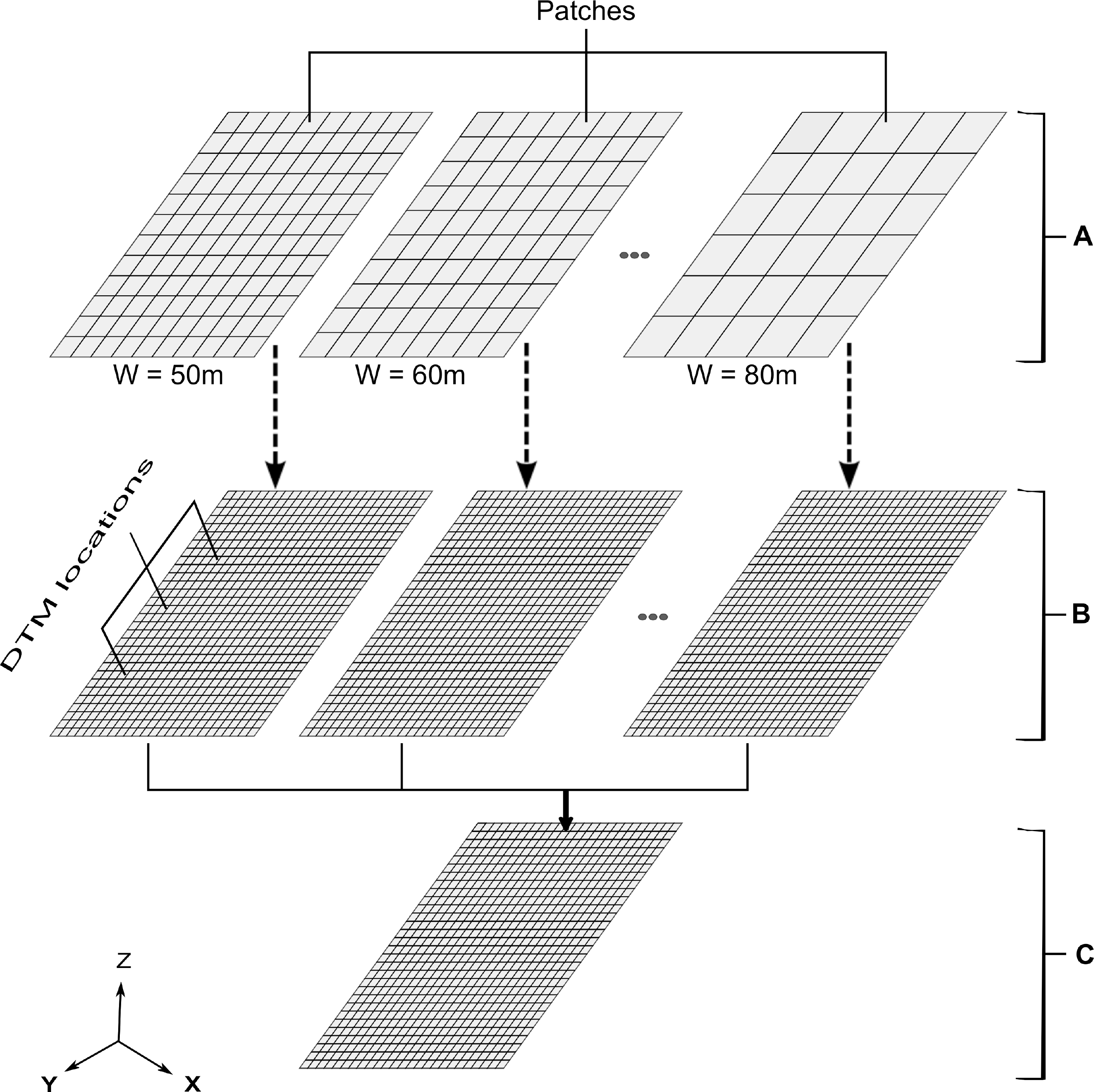
overcome the problems of low data density and the lack of overlapping between DTM patches by iteratively generating a series of coarse DTMs (repeated sampling) using patch widths of varying sizes and combining the coarse DTMs to form the final DTM;

(ii)

develop an interpolation strategy for estimating elevation values at places where both spline and trend surface interpolation fail (gap-filling); and

(iii)

compare the performance of the proposed algorithm with two other algorithms for generating DTMs in forested terrain using data sets from three different tropical test sites, which are characterized by both low point density and varying degrees of terrain roughness.

This approach has the advantage that it helps to deal with low data density by creating a cloud of elevation values using the available data, from which the final DTM is generated. Moreover, in places of extremely low numbers of ground points, approximation is done using a suitable gap-filling algorithm.

2. Material and Methods

2.1. Study Area

This study spans three test sites on three different continents, namely Nepal (Site 1), Brazil (Site 2) and Ghana (Site 3). The three forest types studied in the article were chosen on the principle that they represent typical dense tropical forest types on three different continents. All three LiDAR samples have been collected for a different purpose, as described below.

2.1.1. Site 1

This site consists of three watersheds, namely, Kayarkhola, Charnawati and Ludikhola. The three watersheds cover an area of approximately 27,789 ha. The terrain in the site is predominantly mountainous and complex, consisting of steep slopes and valleys. Altitude in the area varies from 245 m (Kayarkhola) to 3549 m (Charnawati). The average slope in the area is 29.7%, while the maximum slope is 57.3%. The percentage of ground hits in this site is approximately 29.3%.

This site is part of a pilot project for measuring and monitoring carbon stocks in community forests. The aim of the project is to design and set up a governance and payment system for Nepal’s community forest management under the Reducing Emissions from Deforestation and Forest Degradation (REDD) payment scheme for developing countries.

The forest tested in the current article lies on mountainous highland and represents steep orographic variation under a dense canopy. The forest itself is looked after by a local community forest program and has grown from a degraded state into a high biomass forest.

2.1.2. Site 2

This site is part of the Brazilian Amazon. The terrain in the area is predominantly flat with thick forest cover. The point density of LiDAR capture is quite high, amounting to some 14 points per m². Despite such unusually high point density and the corresponding relatively low flying altitude, the number of ground hits is quite low, thereby making DTM generation a challenge. The percentage of ground hits in this site is approximately 2.2%.

The forest in this site is by far the densest of all three, but like much of the Amazonian Forest, it lies on relatively flat land, with local undulation only. The Brazilian sample is from a natural forest, and it was collected for studying the ability of LiDAR to penetrate a very dense, multi-storied canopy. A very high point density was used in the LiDAR capture in order to make sure that at least some pulses hit the ground.

2.1.3. Site 3

The third site is in southwestern Ghana and represents a West African tropical forest in hilly terrain. The forest is dense, even if the current patch is relatively flat. The percentage of ground hits in this site is approximately 4.54%.

This site is part of a forest and land use inventory scheme for the Ghanaian Forestry Commission (see [40]). It represents a West African closed canopy forest that was inventoried for the sake of land use change analysis. The overall terrain is rugged, but with much less steepness than in the Nepalese case. Forests in the sample are not protected and are used for a variety of purposes by the local population.

2.2. Test Data

Test data used in this study consist of three LiDAR data sets from each of the test sites together with plot-level field measurements of tree heights except for Site 2, where tree height measurement from the ground is not possible.

2.2.1. LiDAR Data

The data were collected to support a LiDAR-assisted Multiresource Programme (LAMP), which is a large-scale method for carbon stock mapping that combines LiDAR sampling and satellite imagery to produce accurate carbon stock maps of areas of interest (see [41]).

Table 1. Parameters of the LiDAR data used in this study.

Parameter	Value
	Site 1	Site 2	Site 3
Projection	UTM	UTM	UTM
Datum	WGS84	WGS84	WGS84
Aerial platform	Helicopter	Helicopter	Fixed wing aircraft
Flying altitude	2200 m AGL	850 m AGL	1300 m AGL
Flying speed	80 knots	124 knots	120 knots
Sensor type	Leica ALS-50 II	Leica ALS-50 II	Leica ALS-50 II
Scan angle	20 degrees	Unknown	13.5 degrees
Sensor pulse rate	52.9 Khz	115.8 Khz	81 Khz
Sensor scan speed	20.4 lines/s	Unknown	47.6 lines/s
Average pulse density	0.8 points/m2	14 points/m2	2 points/m2
Swath width at ground level	1601.47 m	350 m	644 m
Beam footprint at ground level	50 cm	Unknown	31 cm
Date collected	March 2011–April 2011	September 2011	December 2011–January 2012

shows a summary of the parameters of interest about the LiDAR data. Flying altitude refers to the vertical distance of the aircraft from the ground level and should be maintained throughout the flight mission. Because of this requirement, a helicopter is the only way to fly in Site 1, since a fixed wing aircraft cannot rise fast enough to maintain a constant flying altitude and follow the quickly undulating terrain. The data was provided courtesy of Arbonaut Ltd. (Joensuu, Finland) in association with the International Center for Integrated Mountain Development (ICIMOD) (Site 1) of Nepal in raw LASer file format (LAS) (ver. 1.2)format.

2.2.2. Field Measurements

In addition to the LiDAR data, field measurements consisting of tree height estimates for 80 circular plots (radius = 12.62 m) in Site 1 were used. There were no field measurements for Sites 2 and 3. The height of each tree with a diameter at breast height of 5 cm was measured using Vertex IV and Transponder T3 measuring devices.

2.3. Methods

The proposed method for ground filtering and DTM interpolation can be broken down into five steps: (1) repeated DTM sampling; (2) generating gridded DTM samples; (3) generating initial DTM; (4) filling gaps; and (5) generating final DTM. These steps are detailed below.

2.3.1. Repeated DTM Sampling

The repeated DTM sampling step generates a series of DTMs using varying patch widths. The aim of this step is to generate several elevation samples at each candidate DTM location (cell) from which the best are selected to form the final DTM.

Input to this step is the original LiDAR point cloud (in ASCII xyz format). Using the method for ground filtering and DTM interpolation proposed by [39], a series of DTMs is generated using patch widths of varying sizes (see Figure 1).

This procedure results in repeated sampling of elevation values at each candidate DTM location (cell), while, at the same time, creating an overlapping effect between the DTM patches of varying widths. The patch widths used in this study were 50, 60, 70 and 80 m. These values were found to work well in all three test sites and were found by experimenting with values between 30 and 100 m using a ten-meter increment.

While generating the individual DTMs in the repeated DTM sampling step, there are times when the algorithm may fail due to a very low number of data points or gaps in the input data (see [39] for details). When this happens during the repeated sampling step, corresponding areas are labeled with a large negative value, so that they can be identified later. We call these bad areas. The magnitude of the value used is roughly twice the average elevation value in the data (see Section 2.3.3 for details).

The output of the repeated DTM sampling step is a series of N DTMs with points created using patch widths of varying widths, where N is the number of sample DTMs created.

2.3.2. Generating Gridded DTM Samples

In this step, a regular grid of desired spatial resolution is generated from each of the sample DTMs generated in the previous step. The purpose of this step is to create candidate DTM locations at the desired resolution, which are common to all the DTM samples and can be aligned easily. Generating gridded DTM samples is done by first creating a grid of regularly spaced points (spaced according to the desired final DTM resolution) in the x-y plane. Next, the created grid is superimposed on each of the sampled DTMs from the previous step, and for each point (x, y) in the regular grid, an elevation value is assigned from the elevation of the closest point in the sampled DTM.

This step produces N gridded DTM samples, each with the same number of aligned grid points (DTM locations), but with possibly different elevation values at corresponding grid points.

2.3.3. Generating Initial DTM

The initial DTM is generated by merging the N gridded DTM samples obtained in the previous step. The merging is done by taking the median of the elevation values from corresponding DTM locations in the gridded DTM samples. For example, in this study, four DTM samples were used, therefore the elevation values at DTM locations in the initial DTM were assigned by taking the median of four elevation values from corresponding DTM locations in the four gridded sample DTMs. Figure 2 illustrates how the merging is done.

When generating the initial DTM by combining the sample DTMs, there are two possible cases: (1) the number of sample DTMs to be combined is odd; and (2) the number of sample DTMs to be combined is even. If the former case prevails, the median of elevation values at corresponding DTM locations happens to be the middle value. In this case, this value is assigned to the corresponding DTM location in the initial DTM regardless of whether this value is a legitimate elevation value or the large negative value used for labeling bad regions. If the latter case prevails, however, the median value will be the average of the two middle elevation values. In this case, it may happen that one or both of the middle values is the special large negative value used for labeling bad regions. It is important at this point to ensure that the resulting median value calculated is negative in order to preserve the identity of bad regions. To meet this condition, the value used for labeling bad regions is chosen to be a negative number with a magnitude of at least twice the average elevation value in the test data. This ensures that if Case 2 prevails, bad regions retain negative elevation values, so that they can be identified in later steps of the algorithm.

The generating initial DTM step results into an initial gridded DTM. The DTM contains negative elevation values (gaps in the DTM) at places where elevation values could not be estimated in the previous steps due to limited number of data points or gaps in the data. The next step is to estimate the elevation values at those places (hereafter referred to as bad regions).

2.3.4. Filling Gaps

In the gap filling step, bad regions in the DTM are filled (repaired) by interpolation. The bad regions can occur at three places in a DTM: (1) completely embedded in the DTM; (2) on the edge of the DTM; and (3) on the corner of the DTM. Figure 3 shows the three possibilities.

The method described here repairs the bad regions that are completely embedded into the DTM and those occurring on the edges. There is not enough information to reliably repair the bad regions occurring at the corners. To repair the bad regions, the following steps are taken:

(i)

locate the next bad DTM location to be repaired;

(ii)

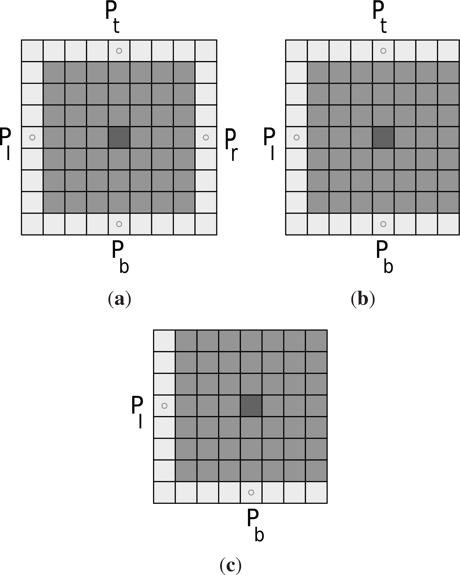
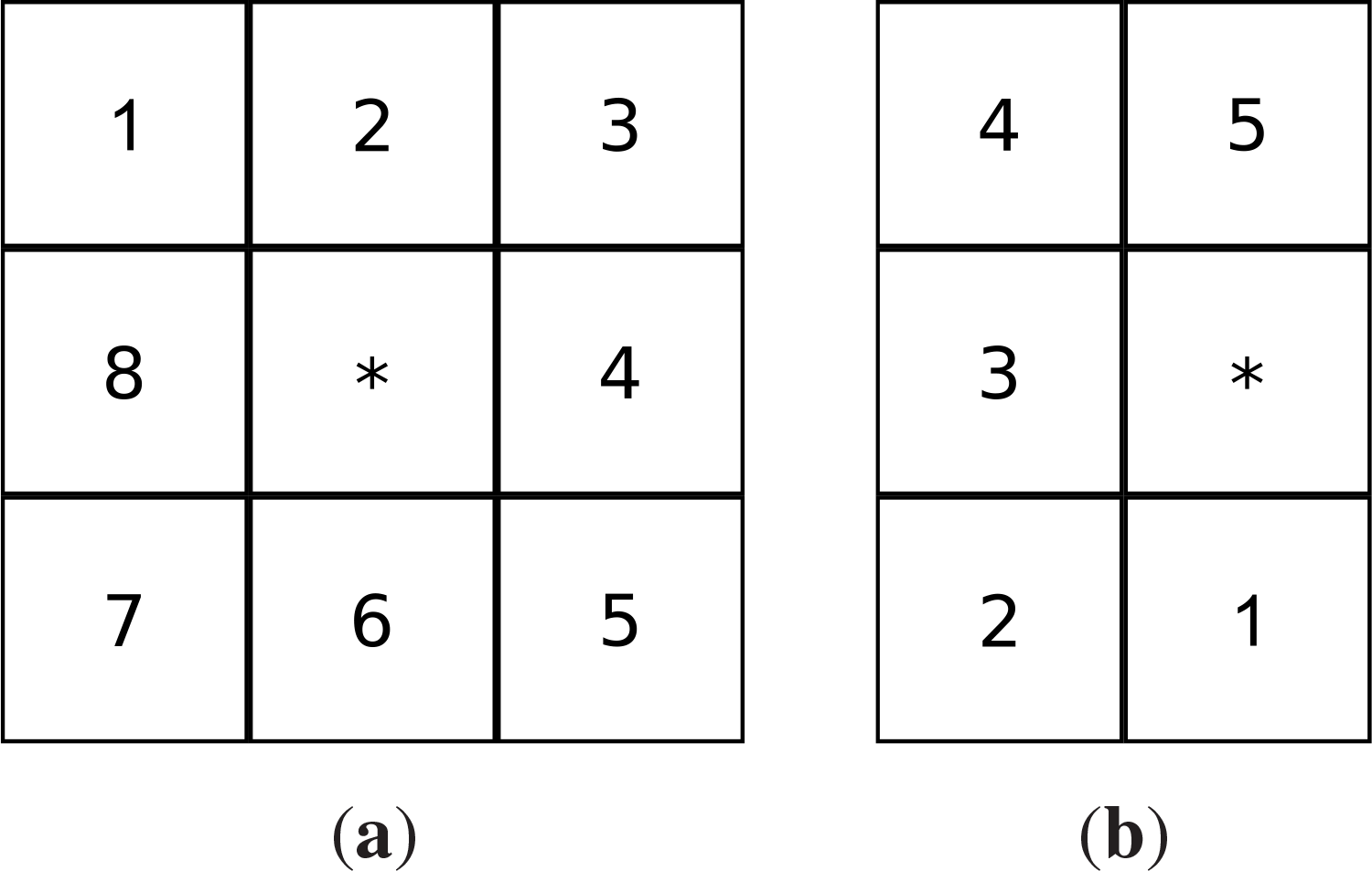
locate the coordinates of the first valid DTM location above the current bad point in the current column (see Figure 4); if none exists, take the x and y coordinates of the topmost point and assign a large positive value (L) for the z coordinate (elevation) and form the top point P_t :(x_t, y_t, z_t); Here, we use the terms above and below with respect to the positions of the points in the vertical direction and the terms left and right with respect to the position of the points in the horizontal direction.

(iii)

Locate the coordinates of the first valid DTM location below the current bad point in the current column (see Figure 4); if none exists, take the x and y coordinates of the bottom most point and assign a large positive value for the z coordinate and form the bottom point P_b :(x_b, y_b, z_b);

(iv)

Locate the coordinates of the first valid DTM location on the left of the current bad point in the current row (see Figure 4); if none exists take the x and y coordinates of the leftmost point and assign a large positive value for the z coordinate and form the left point P_l :(x_l, y_l, z_l);

(v)

locate the coordinates of the first valid DTM location on the right of the current bad point in the current row (see Figure 4); if none exists take the x and y coordinates of the rightmost point and assign a large positive value for the z coordinate and form the right point P_r :(x_r, y_r, z_r);

(vi)

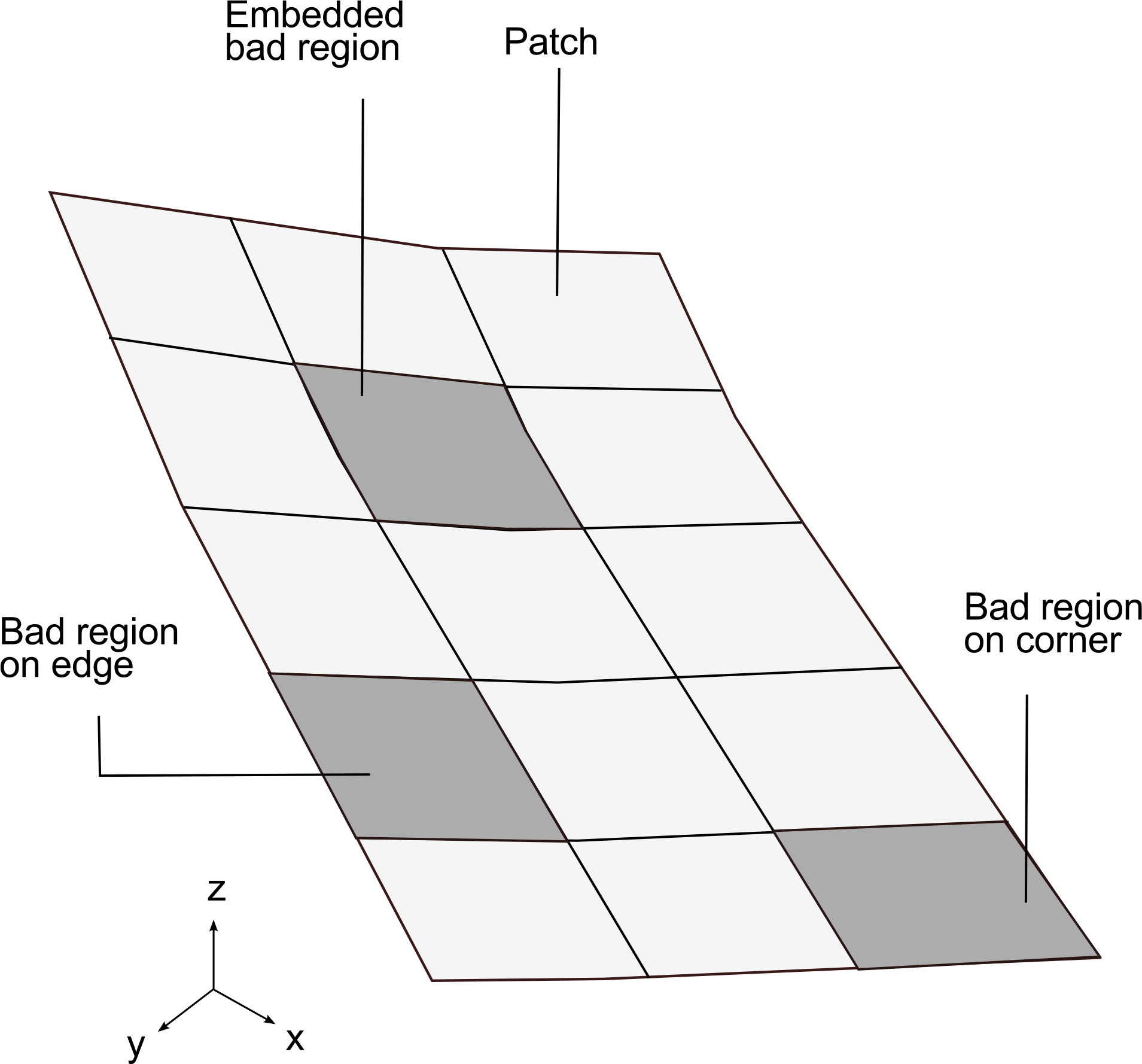
Determine if the bad DTM location is in a bad region lying on a corner by checking if any of the following conditions are true: z_t = z_r = L, or z_t = z_l = L, or z_b = z_l = L, or z_b = z_r = L; if any of these conditions hold, go to Step (i);

(vii)

Determine which direction (vertical or horizontal) has a larger slope (steeper) by comparing the magnitudes of the slopes of the lines segments $\overline{P_b{P}_t}$ and $\overline{P_l{P}_r}$;

(viii)

If the vertical direction is steeper, use the line segment $\overline{P_l{P}_r}$ to interpolate the elevation value at the current bad point, otherwise use the line segment $\overline{P_b{P}_t}$.

The value of L is chosen, such that the slope between the current bad DTM location and the topmost DTM location is considerably larger than the slope between the current DTM location and any other valid DTM location in the DTM. In this study, a value of 10,000 was used, and it was about ten times larger than the average elevation in the data.

The reason for using a line segment in the less steeper direction for estimation is to detect bad regions located on the edges and corners of the DTM and to take appropriate action. This is achieved by the use of the large dummy elevation value described above. For example, if a bad region to be filled is located on either the top or bottom edges of the DTM, then the slope in the vertical direction will be larger than that in the horizontal direction (due to a large elevation value assigned), making the algorithm resort to using a horizontal line segment for estimation. On the other hand, if the bad region is located on either the left of right edges of the DTM, vertical line segments are used for estimation.

Estimating Unknown Elevation Values

After the four points P_t, P_r, P_b and P_l, as well as the direction of a gentle slope have been determined, estimation of the elevation value at the current bad DTM location is done. First, the direction vector v_d is computed using either Equation (1) or Equation (2).

$${\mathbf{v}}_d=P_r-P_l$$

(1)

$${\mathbf{v}}_d=P_t-P_b$$

(2)

Next, using the equation of a line in 3D,

$$\mathbf{p}={\mathbf{p}}_0+t{\mathbf{v}}_d$$

(3)

where p is a general point on the line, p₀ is a known point on the line, t is a parameter and v is a direction vector; the value of the parameter t for line segments $\overline{P_b{P}_t}$ and $\overline{P_l{P}_r}$ is determined using Equation (3) above and available information, i.e., the values of the x and y coordinates of the current bad location and either P_l or P_r if a horizontal line segment is used for estimation; and either P_t or P_b if a vertical line segment is used for estimation. Thus, t is calculated using Equation (4).

$$t=\frac{x-x_t}{{\mathbf{v}}_{d,x}}$$

(4)

where x represents the value of the x-coordinate at the current bad location, x_t represents the x-coordinate of the top point, P_t, and v_d,x represents the x-coordinate of the direction vector, v_d. Alternatively, the same result can be obtained by using the y-coordinates of the vectors involved in Equation (3).

After the value of the parameter t for the interpolating line has been determined, it is used to estimate the elevation value at the current bad location. The estimation is done by using the z-coordinates of the vectors in Equation (3) and using Equation (5).

$$z=z_t+t{\mathbf{v}}_{d,z}$$

(5)

where z is the elevation value being estimated, z_t is the z-coordinate of the top point, P_t, and v_d,z represents the z-coordinate of the direction vector, v_d. Here, the vertical line segment $\overline{P_b{P}_t}$ is being used with P_t as the known point. In a similar fashion, the bottom point P_b can be used or either of the points {P_l, P_r} may be used in case a horizontal line is used for estimation.

2.3.5. Generating the Final DTM

The final step in generating the DTM is to detect and remove jumps (spikes) in the DTM. This is a two-step process. In the first step, jumps are detected and marked, and in the second step, the jumps are removed (repaired). To detect jumps, each DTM location’s elevation is compared with the elevation of its 8 neighbors (for DTM locations not lying on the border) or 5 neighbors (for DTM locations lying on the border) (see Figure 5).

A DTM location is marked as a jump if it fails the test:

$$R<T$$

(6)

where:

$$R=\sum _{i=1}^s\left|Z_i-Z_c\right|$$

(7)

and Z_i represents the elevation value of the neighboring points, Z_c represents the elevation value of the point being tested, s is the upper limit of the summation (8 for the non-border location and 5 for the border locations) and T is a threshold. The value of R is very sensitive to terrain slope, thus a suitable value for T that works well for a particular area and data has to be determined experimentally. In this study, the value of T roughly equal to $\frac{R}{s}$ was found to be suitable in each test area.

After the jumps have been detected and marked, the next step is to repair them. This is done by treating the jumps as small gaps in the DTM and to repair them using the method for filling gaps described in the previous section. Figure 6 illustrates how jumps are detected and repaired.

3. Results and Discussion

In this section, we present the performance results of the proposed algorithm. First, we show how the proposed iterative approach helps to overcome the shortcomings reported in [39], namely, border effects (poor overlapping between patches) and gaps in the DTM in places of extremely low data or the presence of gaps in the data; second, we present results of the relative performance of the proposed algorithm compared with two existing algorithms for the extraction of DTMs from LiDAR data in forested terrain proposed in the literature in [3,4]. We chose to compare our method with these algorithms, because they are in widespread use by the forestry community, both in research and industry.

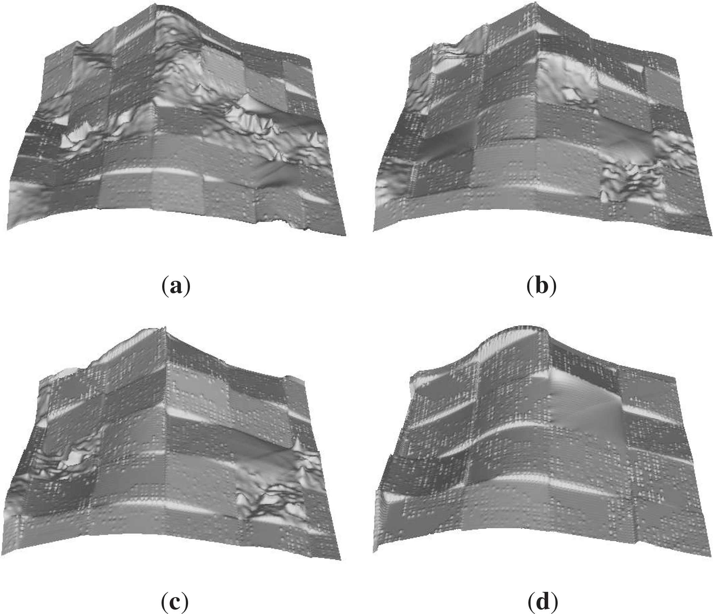
3.1. Minimizing Border Effects

Test results showed that by using patch widths of varying sizes, the problem of a lack of overlap between patches is significantly reduced. As opposed to using only one DTM sample, the use of several DTM samples (repeated sampling) results in the creation of several elevation samples at every DTM location. These elevation samples are produced from DTM samples of different patch widths, thus creating an overlapping effect between the patches of the DTM samples. Figure 7 shows how four DTM samples generated using patch widths varying from 50–80 m at a ten-meter increment are combined to produce the final DTM. Note how the border effects appearing in the four DTM samples are significantly reduced after combining the DTM samples.

Similarly, repeated sampling of elevation values using DTM samples of increasing patch widths helps to overcome the problem of gaps in the DTM resulting from either gaps in the data or low data densities at certain places (due to closed canopy). This problem can be solved in two ways. First, as the patch size is increased, gaps of a relatively small area compared to the patch width get embedded completely or partially into the much larger patches. This is contrary to using a fixed patch width, where small gaps often emerge. Second, gaps in the data are handled by using the gap-filling procedure described in the previous section. This procedure is used to fill gaps that remain before the final DTM is produced. Figures 8 and 9 show how the gap filling algorithm works.

The difference model in Figure 8 shows that the gap filling algorithm works well on flat surfaces (both on slopes and flat terrain), while the accuracy deteriorates with increasing terrain curvature (Figure 9). This is expected behavior, as a substantial amount of information is lost when a hole is located on curved terrain compared to when a hole of the same size is located on flat terrain.

3.2. Comparison with Field Measurements

To assess the accuracy of the algorithm, tree height estimates computed using the algorithm were compared to field-measured tree heights. Computed heights were obtained by first extracting the LiDAR points corresponding to each plot, and the height of the tallest tree in each plot was assumed to correspond to the average of the highest ten LiDAR points.

While comparison of tree heights estimates computed using the algorithm in Site 1 showed a slight improvement against field measurements (RMSE = 1.65 m compared to an RMSE of 1.92 m reported in [39]), the proposed algorithm has shown a significant improvement in dealing with gaps in the data, as well as a low number of ground points. Moreover, the slight improvement in RMSE can be explained by the fact that the field measurements were collected in areas accessible by field measurement crews, i.e., areas with less complex terrain and moderate canopy cover.

3.3. Comparison with Existing Algorithms

We compared the proposed algorithm with algorithms proposed in [3,4]. The comparison was quantitative and was aimed at observing the relative performance of the three algorithms in different kinds of forest cover and terrain type, i.e., the three test sites. This is due to a lack of field ground control data (reference DTMs) in the three test sites. In the following discussion, we are going to refer to the three algorithms as follows. The algorithm proposed by Karl Kraus as KK; the algorithm proposed by Peter Axelsson as PA; and the algorithm proposed in this paper by MA (Maguya Almasi).

In our tests, we used the implementation of KK available in the FUSION software package (see [42]) and that of PA found in the Terrascan software package (see [43]). For details about parameters used to generate the test DTMs from the two software packages; see Appendix A and B. Figures 10 and 12 show a comparison of the three algorithms. The comparison is based on the differences in elevation between the DTMs and the smoothness of the DTMs, and the area covered measures approximately 0.16 square kilometers.

Figure 10 shows that the biggest differences in elevation among the three algorithms occur in Site 1. This observation can be attributed to the fact that, of the three test sites, Site 1 encompasses the most challenging combination of terrain and data for ground filtering algorithms, i.e., it has terrain with steep slopes and low data density. Here, KK seems to perform poorly, whereas PA and MA seem to agree for the most part, with a consistent difference of about 1 m, except for a few places where there is a difference of more than 5 m. These places are the ones in which KK seems to suffer the most (see Figure 10a). The big difference in elevation at these places is due to the closed canopy, which blocks most of the LiDAR pulses. This fools algorithms into misclassifying LiDAR returns from tree branches as ground returns.

In Site 2 PA and MA agree significantly, while KK still presents a significant discrepancy, although not as significant as that observed in Site 1. These differences between the two sites can be attributed to the fact that Site 2 is predominantly flat, less complex terrain. Similar results are observed in Site 3 for PA and MA, while KK continues to deviate.

4. Conclusions

This paper has presented an algorithm for extracting DTMs from LiDAR data in challenging forested terrain. The algorithm overcomes the challenge of low data density under forest canopies by iteratively generating a series of coarse DTMs, which are then combined to form the final DTM.

A comparison with traditional DTM extraction algorithms showed that the performance of the algorithm presented in this paper remained consistent with decreasing data density, while the performance of the traditional DTM extraction algorithms deteriorated with decreasing point density. The main limitation of the proposed algorithm is its inability to reproduce small artifacts in the terrain (e.g., small hills). This is especially true with extremely low data densities, where the sizes of the patches used for local interpolation have to be large enough to get the right amount of ground points for interpolation. Under the challenging circumstances of our three test sites, the quality of the DTM produced clearly outweighs the loss of small features in the terrain. Overall, comparing the ground hit percentages of the three test sites and the challenge they pose to DTM extraction algorithms, it appears that terrain complexity is more detrimental to DTM quality than point density: the Nepalese test site has the most complex terrain, but almost ten times the number of ground hits of the other two test sites, yet it produced the biggest absolute differences between the DTMs.

The proposed algorithm will therefore serve as a base for a new generation of algorithms for DTM extraction in challenging forested terrain. Further work needs to be done to improve the gap-filling method, to find a more robust way to combine the sample DTMs and to conduct further tests on the algorithm.

References

1. Wehr, A.; Lohr, U. Airborne laser scanning—An introduction and overview. ISPRS J. Photogramm. Remote Sens 1999, 54, 68–82. [Google Scholar]
2. Næsset, E. Determination of mean tree height of forest stands using airborne laser sanner data. ISPRS J. Photogramm. Remote Sens 1997, 52, 49–56. [Google Scholar]
3. Kraus, K.; Pfeifer, N. Determination of terrain models in wooded areas with airborne laser scanner data. ISPRS J. Photogramm. Remote Sens 1998, 53, 193–203. [Google Scholar]
4. Axelsson, P. Processing of laser scanner data—Algorithms and applications. ISPRS J. Photogramm. Remote Sens 1999, 54, 138–147. [Google Scholar]
5. Pfeifer, N.; Reiter, T.; Briese, C.; Rieger, W. Interpolation of high quality ground models from laser scanner data in forested areas. Int. Arch. Photogramm. Remote Sens. Spat. Inf. Sci 1999, 32, 31–36. [Google Scholar]
6. Reutebuch, S.E.; Andersen, H.E.; McGaughey, R.J. Light Detection and Ranging(LiDAR): An emerging tool for multiple resource inventory. J. For 2005, 103, 286–292. [Google Scholar]
7. Clark, M.L.; Roberts, D.A.; Ewel, J.J.; Clark, D.B. Estimation of tropical rain forest aboveground biomass with small-footprint LiDAR and hyperspectral sensors. Remote Sens. Environ 2011, 115, 2931–2942. [Google Scholar]
8. Lemmens, M. Airborne LiDAR. In Geo-information; Gatrell, J.D., Jensen, R.R., Eds.; Springer Netherlands: Dordrecht, The Netherlands, 2011; Volume 5, pp. 153–170. [Google Scholar]
9. Full-Waveform Airborne Laser Scanning as a Tool for Archaeological Reconnaissance. Available online: http://w3.riegl.com/uploads/tx_pxpriegldownloads/Doneus_ROME_01.pdf (accessed on 15 July 2014).
10. Ullrich, A.; Studnicka, N.; Hollaus, M.; Briese, C.; Wagner, W.; Doneus, M.; Mücke, W. Improvements in DTM generation by using full-waveform airborne laser scanning data. Proceedings of the 7th International Conference on Laser Scanning and Digital Aerial Photography, Today and Tomorrow, Moscow, Russia, 6–7 December 2007; 6.
11. Jakubowski, M.K.; Guo, Q.; Kelly, M. Tradeoffs between LiDAR pulse density and forest measurement accuracy. Remote Sens. Environ 2013, 130, 245–253. [Google Scholar]
12. Junttila, V.; Finley, A.O.; Bradford, J.B.; Kauranne, T. Strategies for minimizing sample size for use in airborne LiDAR-based forest inventory. For. Ecol. Manag 2013, 292, 75–85. [Google Scholar]
13. Akay, A.; Oguz, H.; Karas, I.; Aruga, K. Using LiDAR technology in forestry activities. Environ. Monit. Assess 2009, 151, 117–125. [Google Scholar]
14. Wang, C.; Glenn, N.F. A linear regression method for tree canopy height estimation using airborne LiDAR data. Can. J. Remote Sens 2008, 34, S217–S227. [Google Scholar]
15. Takahashi, T.; Yamamoto, K.; Senda, Y.; Tsuzuku, M. Estimating individual tree heights of sugi (Cryptomeria japonica D. Don) plantations in mountainous areas using small-footprint airborne LiDAR. J. For. Res 2005, 10, 135–142. [Google Scholar]
16. Van Leeuwen, M.; Nieuwenhuis, M. Retrieval of forest structural parameters using LiDAR remote sensing. Eur. J. For. Res 2010, 129, 749–770. [Google Scholar]
17. Clark, M.L.; Clark, D.B.; Roberts, D.A. Small-footprint LiDAR estimation of sub-canopy elevation and tree height in a tropical rain forest landscape. Remote Sens. Environ 2004, 91, 68–89. [Google Scholar]
18. Yamamoto, K.; Takahashi, T.; Miyachi, Y.; Kondo, N.; Morita, S.; Nakao, M.; Shibayama, T.; Takaichi, Y.; Tsuzuku, M.; Murate, N. Estimation of mean tree height using small-footprint airborne LiDAR without a digital terrain model. J. For. Res 2011, 16, 425–431. [Google Scholar]
19. Nilsson, M. Estimation of tree heights and stand volume using an airborne LiDAR system. Remote Sens. Environ 1996, 56, 1–7. [Google Scholar]
20. Guo, Z.; Fang, J.; Pan, Y.; Birdsey, R. Inventory-based estimates of forest biomass carbon stocks in China. For. Ecol. Manag 2010, 259, 1225–1231. [Google Scholar]
21. Herold, M.; Román-Cuesta, R.; Mollicone, D.; Hirata, Y.; van Laake, P.; Asner, G.; Souza, C.; Skutsch, M.; Avitabile, V.; MacDicken, K. Options for monitoring and estimating historical carbon emissions from forest degradation in the context of REDD+. Carbon Balance Manag 2011, 6, 1–7. [Google Scholar]
22. Avtar, R.; Sawada, H. Use of DEM data to monitor height changes due to deforestation. Arab. J. Geosci 2012, 6, 4859–4871. [Google Scholar]
23. Liu, X. Airborne LiDAR for DEM generation: Some critical issues. Progress Phys. Geogr 2008, 32, 31–49. [Google Scholar]
24. Kraus, K.; Pfeifer, N. Advanced DTM generation from LiDAR data. Int. Arch. Photogramm. Remote Sens 2001, XXXIV-3/W4, 23–30. [Google Scholar]
25. Vosselman, G. Slope based filtering of laser altimetry data. Int. Arch. Photogramm. Remote Sens. Spat. Inf. Sci 2000, XXXIII, 935–942. [Google Scholar]
26. Sithole, G. Filtering of laser altimetry data using a slope adaptive filter. Int. Arch. Photogramm. Remote Sens 2001, XXXIV-3/W4, 203–210. [Google Scholar]
27. Chen, Q.; Gong, P.; Baldocchi, D.; Xie, G. Filtering airborne laser scanning data with morphological methods. Photogramm. Eng. Remote Sens 2007, 73, 175–185. [Google Scholar]
28. Kobler, A.; Pfeifer, N.; Ogrinc, P.; Todorovski, L.; Os̆tir, K.; Dz̆eroski, S. Repetitive interpolation: A robust algorithm for DTM generation from Aerial Laser Scanner Data in forested terrain. Remote Sens. Environ 2006, 108, 9–23. [Google Scholar]
29. Bao, Y.; LiïijŇ, G.; Cao, C.; Li, X.; Zhang, H.; He, Q.; Bai, L.; Chang, C. Classification of LiDAR point cloud and generation of DTM from LiDAR height and intensity data in forested area. Int. Arch. Photogramm. Remote Sens. Spat. Inf. Sci 2008, XXXVII, 313–318. [Google Scholar]
30. Mongus, D.; Z̆alik, B. Parameter-free ground filtering of LiDAR data for automatic DTM generation. ISPRS J. Photogramm. Remote Sens 2012, 67, 1–12. [Google Scholar]
31. Sithole, G.; Vosselman, G. Experimental comparison of filter algorithms for bare-earth extraction from airborne laser scanning point clouds. ISPRS J. Photogramm. Remote Sens 2004, 59, 85–101. [Google Scholar]
32. Hyyppä, H.; Yu, X.; Hyyppä, J.; Kaasalainen, H.; Honkavaara, E.; Rönnholm, P. Factors affecting the quality of DTM generation in forested areas. Int. Arch. Photogramm. Remote Sens. Spat. Inf. Sci 2005, 36, 85–90. [Google Scholar]
33. Holmgren, J.; Nilsson, M.; Olsson, H. Simulating the effects of LiDAR scanning angle for estimation of mean tree height and canopy closure. Can. J. Remote Sens 2003, 29, 623–632. [Google Scholar]
34. Hopkinson, C. The influence of flying altitude, beam divergence, and pulse repetition frequency on laser pulse return intensity and canopy frequency distribution. Can. J. Remote Sens 2007, 33, 312–324. [Google Scholar]
35. Hopkinson, D.; Chasmer, L.E.; Zsigovics, G.; Creed, I.F.; Sitar, M.; Treitz, P.; Maher, R.V. Errors in LiDAR ground elevation and wetland vegetation height estimates. Int. Arch. Photogramm. Remote Sens. Spat. Inf. Sci 2004, 36, 108–113. [Google Scholar]
36. Takahashi, T.; Yamamoto, K.; Miyachi, Y.; Senda, Y.; Tsuzuku, M. The penetration rate of laser pulses transmitted from a small-footprint airborne LiDAR: A case study in closed canopy, middle-aged pure sugi (Cryptomeria japonica D. Don) and hinoki cypress (Chamaecyparis obtusa Sieb. et Zucc.) stands in Japan. J. For. Res 2006, 11, 117–123. [Google Scholar]
37. Fisher, P.F.; Tate, N.J. Causes and consequences of error in digital elevation models. Prog. Phys. Geogr 2006, 30, 467–489. [Google Scholar]
38. Meng, X.; Currit, N.; Zhao, K. Ground filtering algorithms for airborne LiDAR data: A review of critical issues. Remote Sens. 2010, 2, 833–860. [Google Scholar]
39. Maguya, A.; Junttila, V.; Kauranne, T. Adaptive algorithm for large scale dtm interpolation from LiDAR data for forestry applications in steep forested terrain. ISPRS J. Photogramm. Remote Sens 2013, 85, 74–83. [Google Scholar]
40. Sah, B.P.; Hämäläinen, J.M.; Sah, A.K.; Honji, K.; Foli, E.G.; Awudi, C. The use of satellite imagery to guide field plot sampling scheme for biomass estimation in Ghanaian forest. ISPRS Ann. Photogramm. Remote Sens. Spat. Inf. Sci 2012, I-4, 221–226. [Google Scholar]
41. Gautam, B.; Peuhkurinen, J.; Kauranne, T.; Gunia, K.; Tegel, K.; Latva-Käyrä, P.; Rana, P.; Eivazi, A.; Kolesnikov, A.; Hämäläinen, J.; et al. Estimation of forest carbon using LiDAR-Assisted Multi-Resource Programme (LAMP) in Nepal. Presented at International Conference on Advanced Geospatial Technologies for Sustainable Environment and Culture, Pokhara, Nepal, 12–13 September 2013.
42. McGaughey, R.J.; Carson, W.W. Fusing LiDAR data, photographs, and other data using 2D and 3D visualization techniques. Proceedings of Terrain Data: Applications and Visualization—Making the Connection, Charleston, SC, USA, 28–30 October 2003; pp. 16–24.
43. Terrascan. Terrasolid’s Software for LiDAR Data Processing and 3D Vector Data Creation, 2012. Available online: http://www.terrasolid.com/products/terrascanpage.html (accesed on 28 January 2014).
Appendix
A. Parameters Used to Generate Test DTMs in Terrascan
The following parameters were used to generate the test DTMs used for comparison in this study:
Class:2 (ground)
Value:triangulated model
Export:whole area
Grid spacing:1 m
Maximum triangle length:700 m
Model buffer:100 m
Outside points:skip
Z decimals:0.123
B. Parameters Used to Generate Test DTMs in FUSION
The following command was used to generate the test DTMs used in this study from FUSION:
Ground filtering:
groundfilter/gparam:−1/wparam:2/tolerance:0.1/iterations:10 <output laser data (LDA) file> 2 <input LAS file>
DTM generation:
gridsurfacecreate/median:8/spike:20 <output DTM file> 2 MM 112 22 <input LDA file>
Figure 1. Example from Site 1 illustrating repeated sampling of elevation values at DTM locations by repeating DTM interpolation using increasing patch widths ranging from 50 to 80 m at increments of 10 m. (a) Patch width = 50; (b) Patch width = 60; (c) Patch width = 70; (d) Patch width = 80.
Remotesensing 06 06524f1
Figure 2. Generating the initial DTM: DTM samples obtained by repeated sampling (A)are converted into gridded DTM samples at the same resolution (B) from which the initial DTM (C) is obtained by taking the median of corresponding DTM locations. W represents the patch width in meters used to generate each of the sample DTMs.
Remotesensing 06 06524f2
Figure 3. Possible locations for bad regions in a DTM.
Remotesensing 06 06524f3
Figure 4. Locating valid DTM locations when repairing bad regions in a DTM: (a) the case when the bad region is completely embedded into the DTM and all of the required points (Pt, Pr, Pb, and Pl)exist; (b) the case when the bad region lies on the border of the DTM and one of the required points is missing; (c) the case when the bad region lies on the corner of the DTM and either of the pair of the required points {Pt, Pr}, {Pl, Pt}, {Pl, Pb} or {Pb, Pr} is missing. The darkest square at the center represents the DTM location, which is currently being estimated within a bad region (the darker squares); the light squares bordering the bad region represent valid DTM locations used for estimation.
Remotesensing 06 06524f4
Figure 5. Two kinds of neighborhoods used to detect jumps in a DTM: (a) 8 neighborhoods; (b) 5 neighborhoods. The asterisk represents the DTM location being tested.
Remotesensing 06 06524f5
Figure 6. Detecting and repairing jumps in the DTM: (a) original DTM section; (b) locations detected as jumps marked (light spots); (c) jumps repaired using the gap-filling approach described in the previous section. The width of each DTM section is approximately 350 m.
Remotesensing 06 06524f6
Figure 7. Combining four DTMs (a) Patch width = 50; (b) Patch width = 60; (c) Patch width = 70; (d) Patch width = 80 generated using different patch widths to produce the final DTM (e) After combining and removing jumps. Each DTM sample measures approximately 350 m in width.
Remotesensing 06 06524f7
Figure 8. Filling gaps in a DTM on a level surface on a steep slope: (a) original terrain before a gap is introduced; (b) after a 40 m by 40 m gap has been introduced; (c) after the gap has been repaired; (d) a difference model showing the error in estimation between the original and estimated elevation values. The slope at this location is approximately 37%.
Remotesensing 06 06524f8
Figure 9. Filling gaps in a DTM on a curved surface on a steep slope: (a) original terrain before a gap is introduced; (b) after a 40 m by 40 m gap has been introduced; (c) after the gap has been repaired; (d) a difference model showing the error in estimation between the original and estimated elevation values. The slope at this location is approximately 33%.
Remotesensing 06 06524f9
Figure 10. Comparing DTMs produced by (a) Karl Kraus (KK), (b) PeterAxelsson (PA) and (c) Maguya Almasi (MA) at Site 1. The width of the DTM section is approximately 400 m. (d) Difference model: KKMA; (e) Difference model: PAMA.
Remotesensing 06 06524f10aRemotesensing 06 06524f10b
Figure 11. Comparing DTMs produced by (a) Karl Kraus (KK), (b) PeterAxelsson (PA) and (c) Maguya Almasi (MA) at Site 2. The width of the DTM section is approximately 400 m. (d) Difference model: KKMA; (e) Difference model: PAMA.
Remotesensing 06 06524f11aRemotesensing 06 06524f11b
Figure 12. Comparing DTMs produced by (a) Karl Kraus (KK), (b) PeterAxelsson (PA) and (c) Maguya Almasi (MA) at Site 3. The width of the DTM section is approximately 400 m. (d) Difference model: KKMA; (e) Difference model: PAMA.
Remotesensing 06 06524f12aRemotesensing 06 06524f12b