An Approach to Persistent Scatterer Interferometry

Abstract

This paper describes a new approach to Persistent Scatterer Interferometry (PSI) data processing and analysis, which is implemented in the PSI chain of the Geomatics (PSIG) Division of CTTC. This approach includes three main processing blocks. In the first one, a set of correctly unwrapped and temporally ordered phases are derived, which are computed on Persistent Scatterers (PSs) that cover homogeneously the area of interest. The key element of this block is given by the so-called Cousin PSs (CPSs), which are PSs characterized by a moderate spatial phase variation that ensures a correct phase unwrapping. This block makes use of flexible tools to check the consistency of phase unwrapping and guarantee a uniform CPS coverage. In the second block, the above phases are used to estimate the atmospheric phase screen. The third block is used to derive the PS deformation velocity and time series. Its key tool is a new 2+1D phase unwrapping algorithm. The procedure offers different tools to globally control the quality of the processing steps. The PSIG procedure has been successfully tested over urban, rural and vegetated areas using X-band PSI data. Its performance is illustrated using 28 TerraSAR-X StripMap images over the metropolitan area of Barcelona.

1. Introduction

Persistent Scatterer Interferometry (PSI) is a powerful group of techniques for deformation measuring and monitoring using interferometric SAR imagery. PSI represents an advanced type of Differential Interferometric SAR (DInSAR) techniques: it is based on large stacks of SAR images and suitable data modelling procedures that make the estimation of different parameters possible. These parameters include the deformation time series, the average displacement rates and the so-called residual topographic error (RTE), also called residual topographic component, which is the difference between the true height of the scattering phase centre of a given point and the height given by the digital elevation (DEM) model used for this point. This latter parameter plays an important role for modelling and geocoding purposes. In this paper, a new approach to PSI processing, which is implemented in the PSI chain of the Geomatics (PSIG) Division of CTTC, is described. The most important work published on PSI algorithms is briefly recalled before describing the PSIG chain (see Section 2).

Different PSI techniques have been proposed in the last decade. The first PSI approach, called Permanent Scatterers technique, was proposed in [1,2]. These works were then followed by a number of other contributions. The Small Baseline Subset (SBAS) technique is one of the most important and well documented PSI approaches [3–7]. A similar approach was proposed in [8]. A PSI method suitable for geophysical applications is described in [9]. In [10] a simplified approach based on stepwise linear functions for deformation and least squares (LS) adjustment is proposed. The Stable Point Network (SPN) and the Interferometric Point Target Analysis (IPTA) are described in [11,12], respectively. In [13] a new algorithm, called SqueeSAR, which can jointly process Persistent Scatterers (PS) and distributed scatterers is proposed. A similar approach based on polarimetric data is proposed in [14]. In [15] a PSI procedure to cover very wide areas is proposed. Further relevant contributions consist in: adapting the LAMBDA method used in GPS to the PSI parameter estimation [16]; the use of adaptive deformation models in PSI [17]; a method to derive the main characteristics of PSs and classify them in main typologies of urban SAR targets [18]. Finally it is worth mentioning the methods based on multidimensional SAR imaging, also known as SAR tomography [19,20].

The PSI X-band data, which are characterized by high phase quality and short wavelength, are highly influenced by the thermal expansion of the imaged objects [21]. Different methods have been proposed to handle the thermal expansion [22–25]. Other works related to X-band PSI are described in [26–28]. An extension of multidimensional SAR imaging to model thermal expansion is treated in [29].

This paper is organized as follows. Section 2 describes the main features of the entire PSIG chain, which consists of three main blocks. Section 3 discusses the first processing block, which includes the candidate CPS selection, 2D phase unwrapping and a phase unwrapping consistency check. Section 3.1 describes the candidate CPS selection in detail. Section 3.2 is focused on the phase unwrapping consistency check, while Section 3.3 describes the main parameters of the candidate CPS selection. Section 4 is devoted to the third processing block. Section 4.1 describes the core part of this block, i.e., the 2+1D phase unwrapping algorithm, while Section 4.2 discusses its main outputs. Section 5 illustrates the entire procedure using a TerraSAR-X dataset that covers the city of Barcelona. Finally, the conclusions are provided in Section 6.

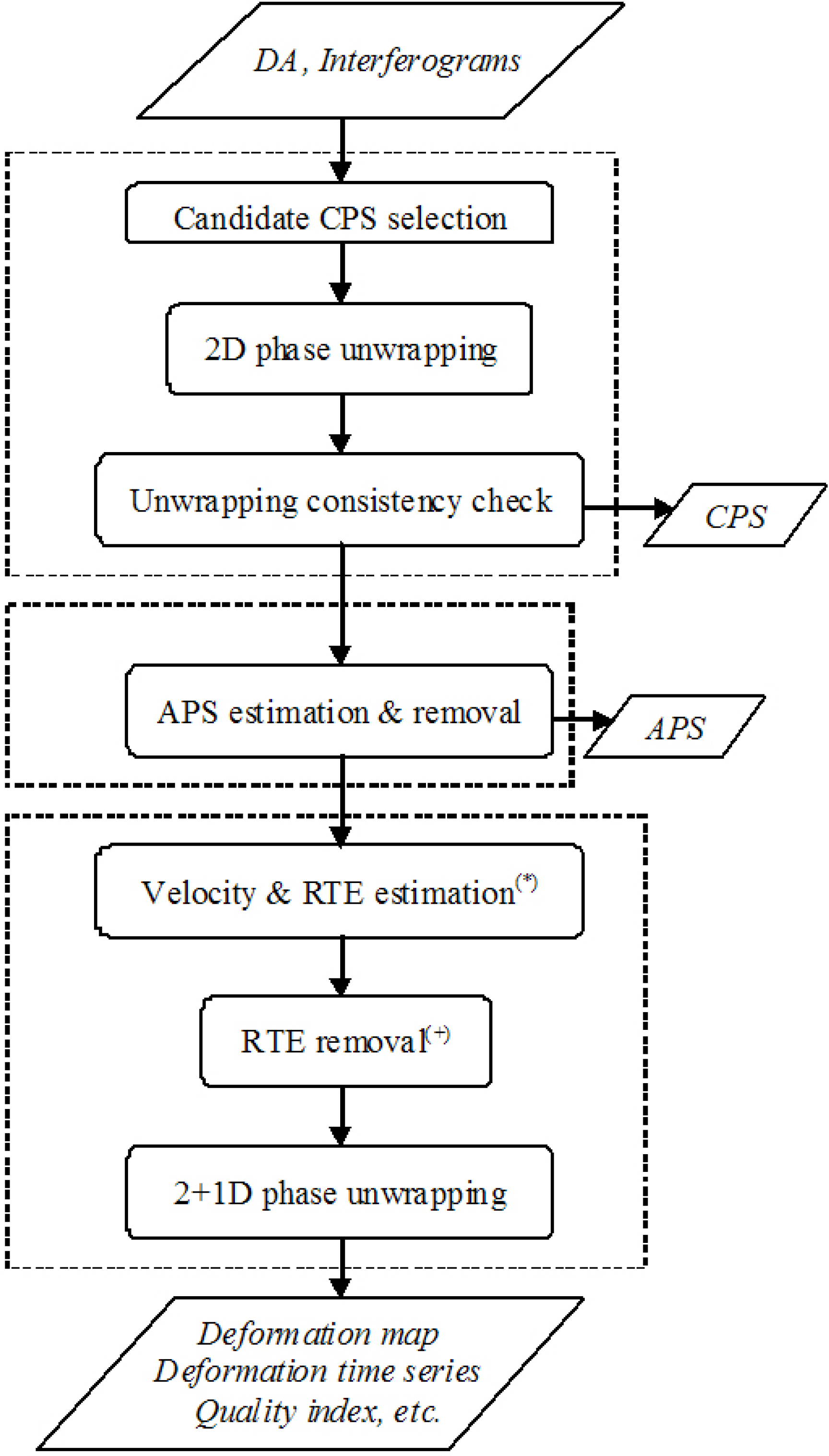
2. The PSIG Procedure

This section describes the key features of the PSIG chain. Its inputs include a stack of N co-registered SAR images, the amplitude dispersion (DA), see [1], and M wrapped interferograms, with M >> N: typically more than 10 interferograms per image are used (a multi-reference procedure is used). The procedure includes three main processing blocks (Figure 1). The goal of the first block is obtaining a set of correctly unwrapped and temporally ordered phases, which are computed on PSs that cover the area of interest with a homogeneous density. In the second block, the abovementioned phases are used to estimate the Atmospheric Phase Screen (APS) using spatio-temporal filters. Finally, the deformation time series are computed on a dense set of PSs in the third block. The main processing steps are briefly described below.

• Candidate Cousin PS (CPS) selection. In this step, a set of PSs with phases characterized by a moderate spatial variation is sought. This is accomplished by using at least a seed PS and searching for its “cousins”, i.e., PSs with similar characteristics (the details are described in the next section). An iterative process is used to ensure an appropriate CPS coverage and density;
• 2D phase unwrapping. 2D phase unwrapping is performed on the candidate CPSs using the redundant set of M interferograms. An implementation of the Minimum Cost Flow method [30,31] is used in this step;
• Phase unwrapping consistency check. This check is based on a LS estimation, followed by the analysis of the so-called residuals (the details are described in the next section). The final set of CPSs is selected at this stage;
• APS estimation and removal. Using the selected CPSs, the APS is estimated using spatio-temporal filters [1–3,8]. The APS is then removed from the original interferograms, obtaining a set of M APS-free interferograms;
• Estimation of deformation velocity and RTE. The deformation velocity and RTE are computed over a dense set of PSs (much denser than the selected CPSs), from the M wrapped APS-free interferograms, using the method of the periodogram [1]. Optionally, an extension of the two-parameter model can be used to account for the thermal expansion [24];
• RTE removal. The RTE phase component is removed from the wrapped APS-free interferograms. The linear deformation component can optionally be removed and then, in a later stage, added back to the deformation time series. The same procedure can be done with the thermal expansion component;
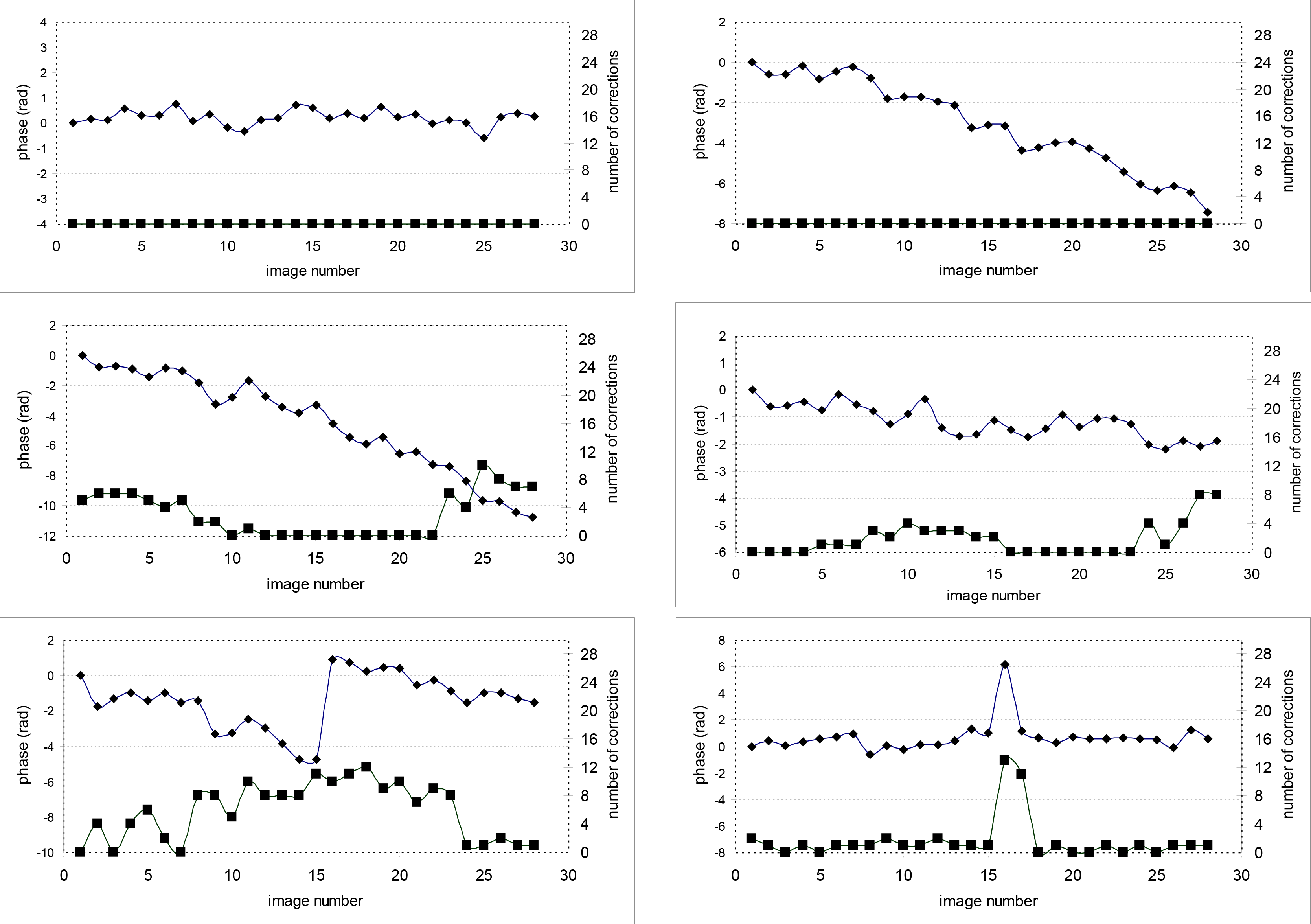
• 2+1D phase unwrapping. A 2+1D phase unwrapping is executed on the set of M APS- and RTE-free interferograms to obtain the final deformation phase time series, a quality index for each time series and other parameters related to the detection and correction of unwrapping errors (detailed information is provided in Section 4.2).

The following sections are focused on the first and the third blocks of the procedure.

3. First Processing Block

The goal of this processing block is obtaining correctly unwrapped and temporally ordered phases over a set of PSs, named CPSs, which have to cover the area of interest with a homogeneous density. This is accomplished through three main steps:

• Candidate CPS selection;
• 2D phase unwrapping on the selected CPSs;
• Phase unwrapping consistency check.

The first and the third steps are discussed in the following sections.

3.1. Candidate CPS Selection

In order to correctly unwrap the interferometric phases, a set of PSs with phases characterized by moderate spatial variations is sought in this step. Let us consider the interferometric phase difference between two pixels i and j, Δφ_ij:

$$\mathrm{\Delta }{\phi }_{i,j}=\mathrm{\Delta }{\phi }_{\mathit{Defo}\_i,j}+\mathrm{\Delta }{\phi }_{\mathit{Ther}\_i,j}+\mathrm{\Delta }{\phi }_{\mathit{RTE}\_i,j}+\mathrm{\Delta }{\phi }_{\mathit{Atmo}\_i,j}+\mathrm{\Delta }{\phi }_{\mathit{Noise}\_i,j}$$

(1)

where Δφ_{Defo_i,j} is the phase difference due to deformation, Δφ_{Ther_i,j} is the phase difference due to thermal expansion, Δφ_{RTE_i,j} is the phase difference due to the RTE, Δφ_{Atmo_i,j} is the phase difference due to the atmospheric component and Δφ_{Noise_i,j} is the difference of the phase noise components. The procedure includes the following steps:

(1)

At least one seed PS is chosen with the following characteristics: φ_{Defo_SEED} = 0, φ_{Ther_SEED} = 0, φ_{RTE_SEED} = 0 and φ_{Noise_SEED} = 0 small. In other words, a PS located on the ground, with no deformation or thermal expansion and characterized by small noise is sought.

(2)

The candidate CPSs are those PSs that satisfy the following condition:

$${\left|\mathrm{\Delta }{\phi }_{i,\mathit{SEED}}^{unw}\right|}_{90\%}<\mathit{Thr}$$

(2)

where ${\left|\mathrm{\Delta }{\phi }_{i,\mathit{SEED}}^{unw}\right|}_{90\%}$ is the 90th percentile of ${\left|\mathrm{\Delta }{\phi }_{i,\mathit{SEED}}^{unw}\right|}^k$, where k runs over the minimum set of N − 1 independent interferograms, where N is the number of images, and Thr is a phase threshold. Before computing their absolute value and ordering them, the $\mathrm{\Delta }{\phi }_{i,\mathit{SEED}}^{\mathit{wrap}}$ values are unwrapped using this simple rule: if $\left|\mathrm{\Delta }{\phi }_{i,\mathit{SEED}}^{\mathit{wrap}}\right|<\pi$ then $\mathrm{\Delta }{\phi }_{i,\mathit{SEED}}^{\mathit{uwr}}=\mathrm{\Delta }{\phi }_{i,\mathit{SEED}}^{\mathit{wrap}}$, if $\mathrm{\Delta }{\phi }_{i,\mathit{SEED}}^{\mathit{wrap}}<-\pi$ then $\mathrm{\Delta }{\mathrm{\Phi }}_{i,\mathit{SEED}}^{\mathit{uwr}}=\mathrm{\Delta }{\mathrm{\Phi }}_{i,\mathit{SEED}}^{\mathit{wrap}}+2\pi$ and if $\mathrm{\Delta }{\mathrm{\Phi }}_{i,\mathit{SEED}}^{\mathit{wrap}}>\pi$ then $\mathrm{\Delta }{\phi }_{i,\mathit{SEED}}^{\mathit{uwr}}=\mathrm{\Delta }{\phi }_{i,\mathit{SEED}}^{\mathit{wrap}}-2\pi$. The use of the 90th percentile confers robustness to the filter: it can cope with up to 10% of outliers. The threshold is discussed in the following section. This operation is repeated for all the PSs that fall within a given window, which is centred on the seed. The window size (Win) is set to have relatively small values of Δφ_{Atmo_i,j}. It is worth noting that the above condition is more restrictive than the ones based on the classical two-parameter model (mean deformation velocity and RTE), see [32,33]. However, the proposed procedure is computationally lighter than the one based on the two-parameter model.

(3)

This operation is repeated recursively, using a given candidate CPS as seed, until the area of interest is sufficiently covered by CPSs. Additional seeds might be required to cover isolated areas or to increase the CPS density in a given area.

2D phase unwrapping is performed on the set of candidate CPSs using the redundant set of M interferograms.

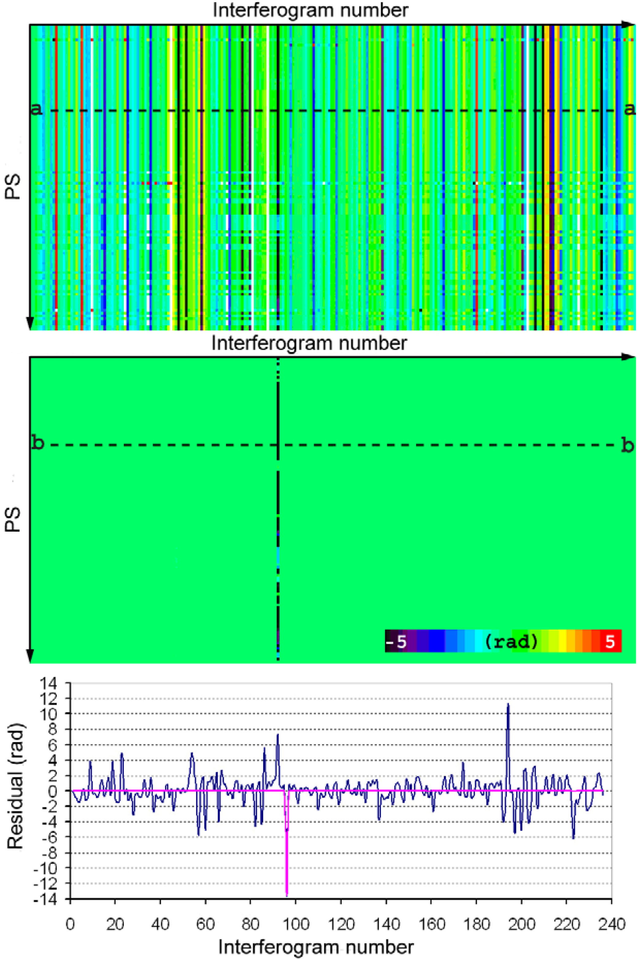
3.2. Phase Unwrapping Consistency Check

In the previous step, the unwrapped phases estimated on the set of candidate CPSs are obtained. A further selection is performed in this step to obtain the selected CPSs. This is done using a phase unwrapping consistency check based on the following observation equation:

$$\mathrm{\Delta }{\phi }_{MS}={\phi }_S-{\phi }_M$$

(3)

where Δφ_MS is the unwrapped interferometric phase (the observation), S and M are the slave and master images (the unknowns). The lth image contains the following phase components:

$${\phi }_l={\phi }_{\mathit{Defo}\_l}+{\phi }_{\mathit{Ther}\_l}+{\phi }_{\mathit{Atmo}\_l}+{\phi }_{\mathit{RTE}\_l}+{\phi }_{\mathit{Noise}\_l}$$

(4)

where φ_{Defo_l} is the deformation component, φ_{Ther_l} is the thermal expansion component, φ_{Atmo_l} is the atmospheric component, φ_{RTE_l} is the RTE component and φ_{Noise_l} is the phase noise. M equations with N − 1 unknowns written for each pixel: the phase of the first image φ₀ is set to zero because Equation (3) has a datum defect: it is translation-invariant. The system of observation equations can be written as:

$$b=A\cdot x$$

(5)

where b = (Δφ_0l, …, Δφ_ij, …, Δφ_{m(N − 1)})^T is the M-dimensional observation vector, A is the design matrix that expresses the set of scalar Equations (3) in matrix form and x = (φ₁, …, φ_i, …, φ_j, …, φ_{N − 1})^T is the N-1-dimensional vector of unknowns. A stochastic model is associated with the functional model in Equation (5), which is represented by weight matrix P. Usually, the observations are equally weighted. The LS solution is given by:

$$\begin{array}{c}\stackrel{⌢}{x}=-{(A^t\cdot P\cdot A)}^{-1}\cdot A^t\cdot P\cdot b\\ \stackrel{⌢}{b}=A\cdot \stackrel{⌢}{x}\\ {\stackrel{⌢}{\phi }}_{\mathit{res}}=b-\stackrel{⌢}{b}\end{array}$$

(6)

where x̆ is the vector of estimated unknowns, b̆ is the vector of the a posteriori estimated observations and ̆_res is the vector of residuals.

A candidate CPS is finally selected as CPS if its vector of residuals satisfies this condition:

$${\stackrel{⌢}{\phi }}_{\mathit{res}}=\overrightarrow{0}$$

(7)

This condition is only valid for data at full resolution. The equivalent condition with multi-look data is having all the residuals sufficiently small. It is worth emphasising that this second filter is highly automated. After this, a check of the distribution of the CPSs is usually carried out to ensure a homogeneous density over the entire area of interest. If this is not accomplished, the procedure is resumed using new seeds to look for new candidate CPSs.

3.3. Candidate CPS Selection: Main Parameters

The parameters used in the candidate CPS selection are discussed in this section. The most important is Thr. The choice of this value is a trade-off between low phase variation, which ensures a correct phase unwrapping, and the need to connect all the parts of a given area of interest. The latter aspect is critical when the area of interest includes rural and vegetated areas where the PS density can be very low. By contrast, it is not very relevant in urban areas, where the choice of Thr can be very restrictive. This can have some interesting applications, as selecting all the PSs that are on the ground or, in general, selecting all the PSs located at a given height, which can be fixed through the seed PS. For instance, in the Seattle dataset mentioned in

Table 1. Main characteristics of the three datasets considered in this work.

Dataset	# Images	# Seed PSs	Area (km2)	Candidate CPSs	Candidate CPS Density (PS/km2)	Selected CPSs (%)
Barcelona	28	9	1019	611,813	600	87
Burgos	11	1	113	82,841	733	74
Seattle	30	5	365	34,594	95	82

, with 30 images and perpendicular baselines distributed between [−800; 600 m], using Thr = 0.7 rad all candidate CPSs obtained were basically located on the ground, with heights below 2 m.

The candidate CPS selection approach was successfully tested over urban, rural and vegetated areas using X-band PSI data. Its performances are illustrated considering three PSI datasets, (Table 1): the Barcelona (Spain) dataset, which covers the full frame of a stack of TerraSAR-X Stripmap images (1019 km²), the Burgos (Spain) dataset, which covers 113 km² and is based on TerraSAR-X Stripmap images, and the Seattle dataset, which consists of CosmoSkyMed Stripmap images and covers an area of 365 km² around the city of Seattle (USA). The three datasets were processed using Win = 400 pixels and Thr defined as a function of the distance from the seed (D), which was computed using these values: 0.8 rad with D = 0 m, 1.1 rad with D = 100 m, 1.35 rad with D = 200 m, 1.52 rad with D = 300 m. To the authors’ experience, working with X-band data, a maximum Thr of 0.8 rad, with D = 0 m, should be used. The increase of Thr with the distance takes into account the term Δφ_{Atmo_i,j} from Equation (1): its values were derived by analysing the average autocorrelation function of the atmospheric component of the Stripmap SAR images of the Barcelona dataset. In order to speed up the computation, the CPS selection was restricted to all PSs with DA smaller than 0.3.

In the Barcelona dataset, 611,813 candidate CPSs were found, covering an area of 1019 km² with a density of 600 candidate CPS/km², using nine seeds; 87% of the candidate CPSs satisfied the filter from Equation (7) and became selected CPSs. In the Burgos dataset, 82,841 candidate CPSs were found over an area of 113 km², with a density of 733 candidate CPS/km², from one seed. The higher density is mainly attributable to the smaller number of images of this dataset. Seventy-four percent of the candidate CPSs were selected as CPSs. Finally, in the Seattle dataset, 34,594 candidate CPSs were found in an area of approximately 365 km², with a density of 95 candidate CPS/km², from five seeds. The remarkably reduced density is not due to the different sensor (CosmoSkyMed): it is caused by the wide perpendicular baseline distribution of this dataset, [−800; 600 m] with respect to the distribution of the Barcelona dataset [−170, 150 m]. In this case, 82% of the candidate CPSs were selected as CPSs. It is worth noting that an alternative approach to CPS selection could be used, by explicitly modelling the phase component due to RTE. This would allow us to obtain more CPSs. However, this approach would require more complex, multi-baseline model assisted, phase unwrapping algorithms.

4. Third Processing Block

The deformation velocity and time series are estimated for a dense set of PSs from the APS-free interferograms in the third processing block. This block involves three main steps:

• Estimating the deformation velocity and RTE and, optionally, the thermal expansion;
• Removing the RTE component from the APS-free interferograms. The deformation velocity and the thermal expansion components are optionally removed;
• Performing the 2+1D phase unwrapping.

The following two sections are focused on the 2+1D phase unwrapping algorithm and its main outputs.

4.1. 2+1D Phase Unwrapping

The procedure starts with a set of M APS- and RTE-free interferograms. The proposed method works with redundant networks: typically more than 10 interferograms per each of the N images are used. The first step is 2D phase unwrapping, which is performed separately on each interferogram using the Minimum Cost Flow method [30,31]. The temporal component of the M interferograms is then exploited in a second step, through a 1D phase unwrapping, which is performed pixel wise. For this reason, the entire procedure is named 2+1D phase unwrapping. The 2D phase unwrapping represents a critical and error-prone processing stage. The phase unwrapping errors, which are integer multiples of 2π, can be caused by different factors as phase noise, high local deformation gradients, strong atmospheric phase component, especially for isolated pixels, etc.

The main goal of the 1D phase unwrapping is the detection and correction of the errors generated in the 2D phase unwrapping stage. For this purpose, it uses an iterative LS procedure [34–36] which fully exploits the integer nature of the unwrapping errors. It is worth emphasising that the SVD algorithm, useful to join non-connected subsets of interferograms [3], is not used. In fact, as mentioned above, a unique set of hyper-connected images and interferograms, for which the SVD is not necessary, is used.

The 1D phase unwrapping involves a pixel wise procedure based on Equations (3) and (4). There are two key parameters that drive the 1D phase unwrapping. The first one is the residual φ_res associated with a given observation:

$${\phi }_{\mathit{res}}=\mathrm{\Delta }{\phi }_{MS}-({\stackrel{⌢}{\phi }}_S-{\stackrel{⌢}{\phi }}_M)$$

(8)

where φ̆_M and φ̆_S are the a posteriori LS estimated image phases. The second parameter is the redundancy of the network of interferograms and images. For each image, it is important to consider the number of interferograms that are directly tied to it, i.e., the number of interferograms where the given image appears either as master or slave. The main steps of the 1D phase unwrapping algorithm include:

(1)

Performing the first LS estimation, computing the residuals (Equation (6));

(2)

Temporally removing the highest absolute residual (outlier candidate) from the network, and performing a new LS estimation;

(3)

Checking the residual of the outlier candidate: if it is a multiple of 2π (within a given tolerance), the observation is corrected and reaccepted. In this way, it is possible to correct the unwrapping errors. Otherwise, the decision of re-entering or rejecting the outlier candidate is based on the comparison of its old and new residuals;

(4)

Performing a new LS estimation, computing the residuals and restarting the procedure from point (2). The procedure is executed iteratively from points (2)–(4) until there are no remaining outlier candidates, i.e., there is no residual above a given threshold. Then, the correction of the unwrapping-related errors is extended to all the residuals that, within a given tolerance, are multiples of 2π.

The core of the proposed algorithm is given by the so-called redundancy matrix R. The LS is not a robust estimation method, considering that a given error is spread out through the network according to the characteristics of A and P. In order to identify correctly the residuals that are multiple of 2π, it is necessary to analyse how the errors are distributed in the network. This is contained in the redundancy matrix R [35]:

$$R=I-A\cdot {(A^t\cdot P\cdot A)}^{-1}\cdot A^t\cdot P$$

(9)

R is only related to A and P, i.e., it is not affected by the observation vector. This matrix is used to correct the LS residuals by the redundancy of the corresponding observations:

$${\stackrel{⌢}{\phi }}_{\mathit{res}\_h}^{*}=\frac{{\stackrel{⌢}{\phi }}_{\mathit{res}\_h}}{r_{hh}}$$

(10)

where ${\stackrel{⌢}{\phi }}_{\mathit{res}\_h}^{*}$ is the corrected hth residual and r_hh is the hth diagonal element of R, which is called the local redundancy. The procedure to correct the unwrapping errors explained above is performed on the corrected residuals. If there is sufficient system redundancy, the LS spreading of errors is mitigated and the unwrapping errors are properly identified. However, it is worth emphasising that this requires that the majority of the interferograms connected to a given image are correctly unwrapped. The algorithm checks the available local redundancy at each iteration and leaves a given outlier candidate untouched if its redundancy is too low. If this occurs, the corresponding parts of the network have to be checked off-line after concluding the automatic analysis. That is, the 1D phase unwrapping only works over the redundant parts of the analysed network. This is often a limitation in the case of ERS and Envisat images where, due to the dispersion of baselines, it is often difficult to obtain a unique and hyper-connected set of interferograms. By contrast, this is not a problem with X-band data and, more importantly, it will not be a problem with the Sentinel-1 data.

The above procedure generates a rich set of parameters. The vectors of residuals for all the analysed pixels, computed at the first and last iterations, are useful to obtain an overview of the entire dataset. In particular, they can be used to identify anomalous interferograms or images, where clusters of high residuals typically occur. An example is illustrated in the following section. The main 1D phase unwrapping output is a phase time series per each analysed pixel, a quality index and the number of corrections per each image. These outputs are discussed in the next section.

4.2. 2+1D Phase Unwrapping: Description of the Outputs

This section describes the main outputs of the 2+1D phase unwrapping. A key output is given by the plots of the LS residuals at the first and last iterations (Figure 2). The plot at the first iteration is useful to obtain an overview of the distributions of phase unwrapping errors, both interferogram wise and PS wise. Figure 2(top) shows the distribution of the residuals for a group of PSs: it is perceptible that they are characterized by a similar pattern. Note that during the phase unwrapping consistency check (Section 3.2), the same plot is used, imposing that all the residuals equal to zero for all interferograms of a given candidate CPS. The plot of the last iteration usually displays zero values, unless there are problematic interferograms, e.g., like the one shown in Figure 2(middle): all PSs have high residuals in correspondence to the same interferogram. In this specific case, the anomalous interferogram was removed from the network and the 1D phase unwrapping was executed again.

Another important output is given by a three-class quality index associated with each deformation time series. Three classes are defined, “Good”, “Fair” and “Warning”, which are derived per each image of a given time series by computing the ratio (Cor_%) between the corrections and the interferograms connected with the image at hand. “Good” indicates that Cor_% is less than 30% for all the images; “Fair” is when Cor_% is between 30% and 40%; and “Warning” is when at least one image has Cor_% above 40%.

In addition to the quality index, the corrections per image are obtained for each time series. This is the most complete information that can be used to assess the quality of each image of a given time series. Some examples are shown in Figure 3. In this case, the 1D phase unwrapping was performed using a network of 28 images and 27 interferograms per image. Figure 3(top) shows two examples of “Good” time series, where zero corrections were applied during the 1D phase unwrapping. One time series shows a stable PS, while the other one displays a displacement away from the sensor. Figure 3(middle) shows two “Fair” time series, while Figure 3(bottom) shows two “Warning” time series. These latter two time series show aliasing. On the left side, the aliasing occurs between the 15th and 16th images and affects half of the time series, while on the right side the corrections basically affect two images (16th and 17th) and the aliasing is only localized in one image. It is worth noting that the aliasing does not occur in every “Warning” time series. This last example illustrates how the corrections are useful to discriminate between the most reliable and problematic images within a given time series.

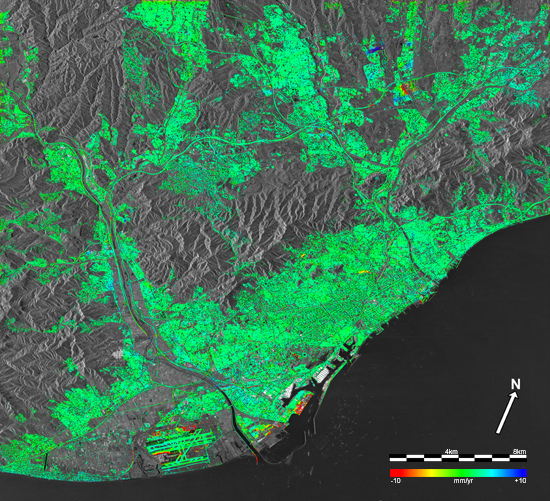
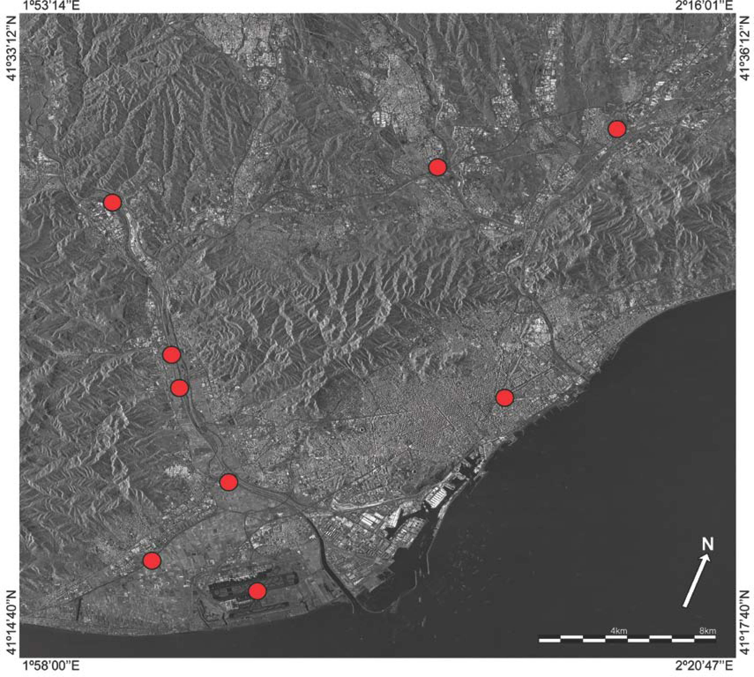
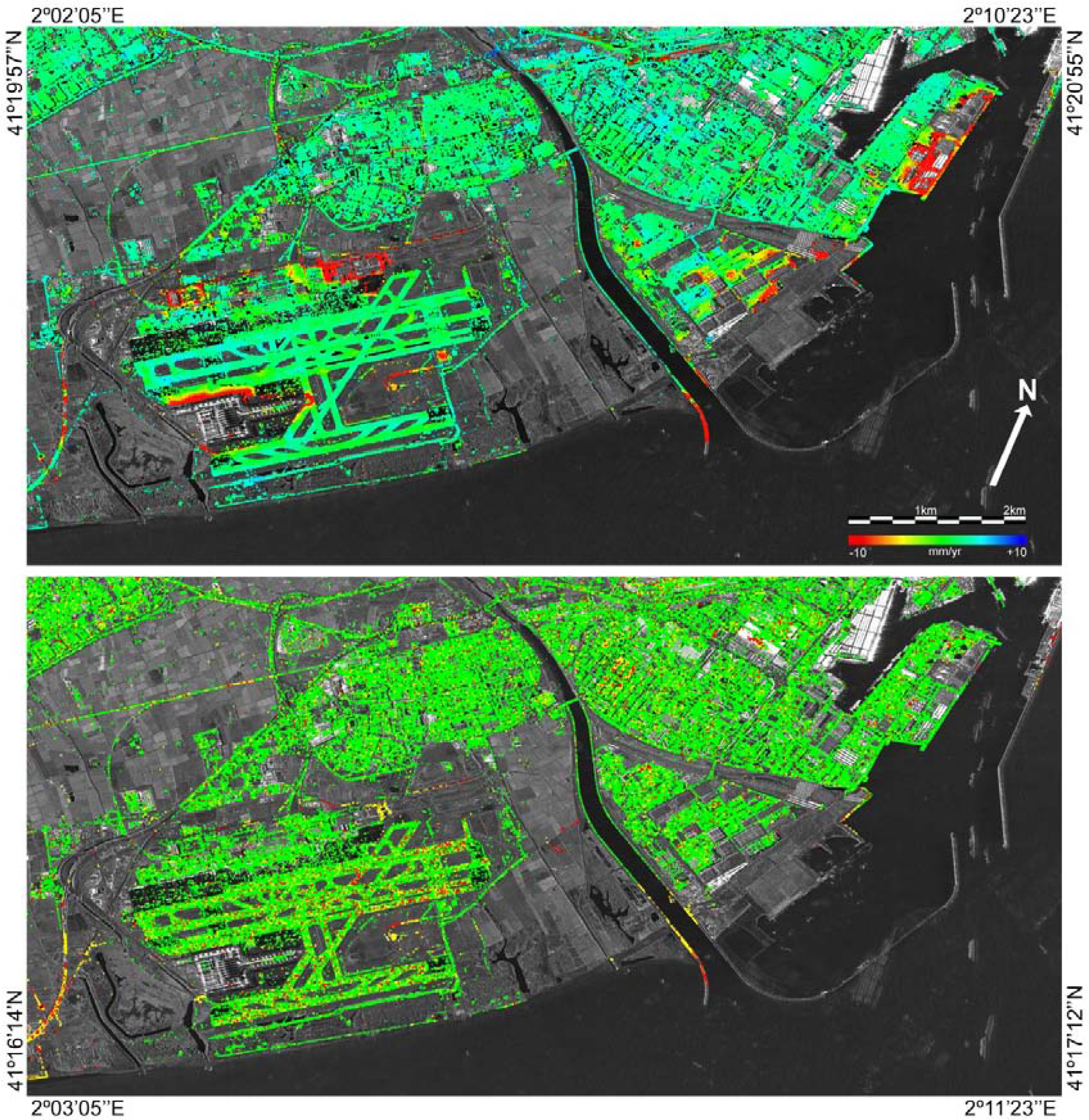
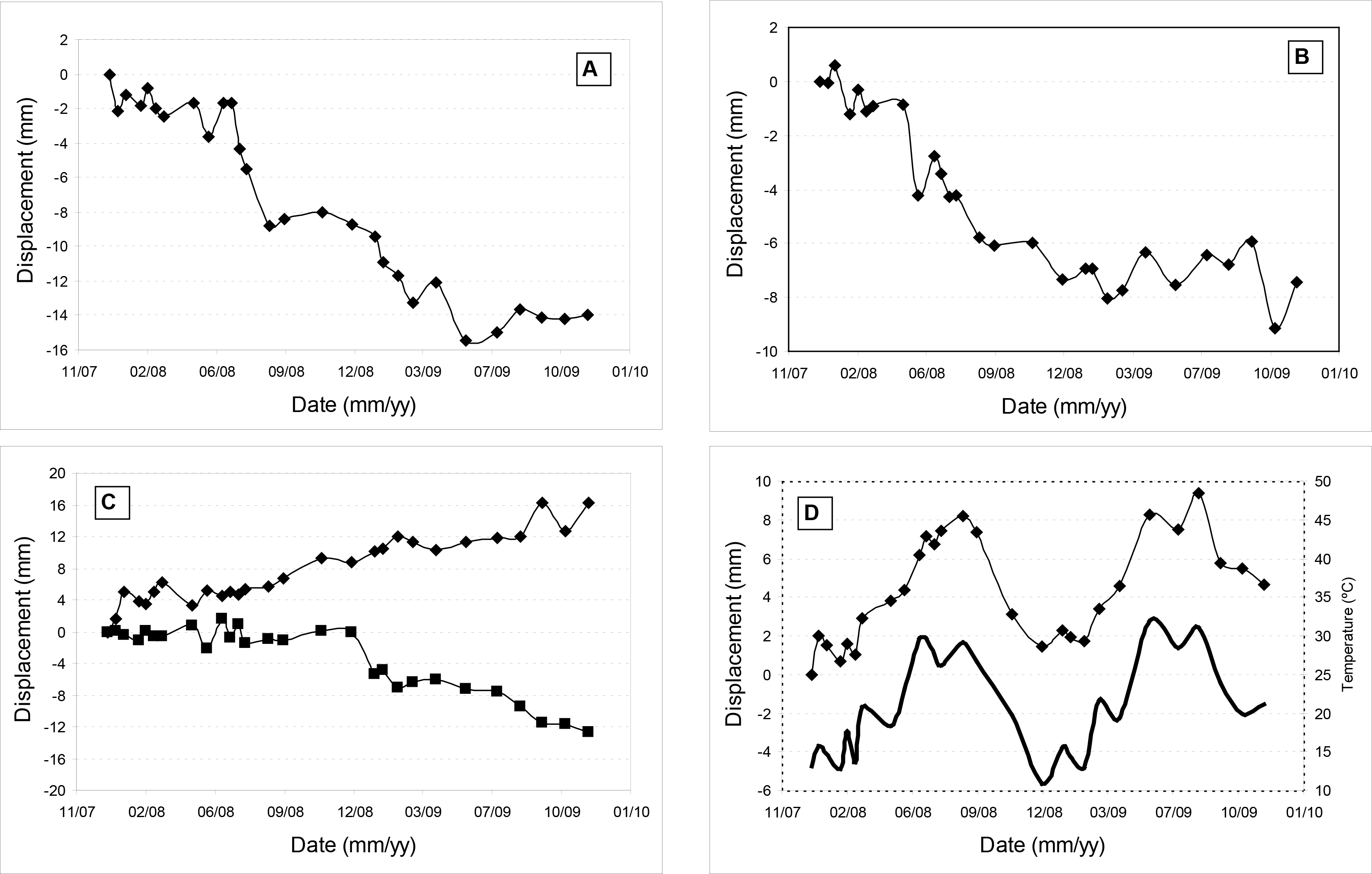
5. Analysis of the Barcelona Dataset

This section describes the results obtained using the Barcelona dataset, already mentioned in Section 3.3 and Table 1. The dataset includes 28 images and 375 interferograms (almost the full set of possible interferograms was used) that cover the period from December 2007 to November 2009. The candidate CPS selection, which was based on nine seed PSs evenly distributed in the image frame (Figure 4), found 611,813 candidate CPSs. It is worth noting that the selection of a similar set of PSs using the classical two-parameter model (mean deformation velocity and RTE) would have required a more complex data processing. In fact, the CPS selection is more straightforward and flexible because it makes use of a set of non-connected CPS networks (in this specific case, nine networks generated from the nine seeds). By contrast, the two-parameter model requires the connection of all PSs in a unique network. An additional advantage is that in the two-parameter model the mean deformation velocity and RTE may be severely affected by the atmospheric effects, which are particularly strong using X-band data, while this does not occur in the candidate CPS selection.

The deformation velocity map of the full frame image is shown in Figure 5. It comprises more than 5.4 million PSs and covers 1019 km². Only the major deformation phenomena are visible in this image: the airport and the port of Barcelona and other subsidence and uplift areas located at the top right part of the image. However, more than 30 major deformation phenomena were found over the entire frame. Although not all of them have been analysed yet, there are several examples of deformation due to soil compaction, water abstraction, landslides, underground construction works (metro line and metro stations), etc. These results represent a valuable source of information for the public and private entities in charge of the maintenance of indispensable assets of the Barcelona metropolitan area.

Figure 6 shows a zoom of Figure 5 over the airport and port area, where several structures and infrastructures affected by deformation phenomena are visible. In the same figure, the quality index map of the same area, which is useful to obtain a preliminary and concise overview of the quality of the estimated PSs, is displayed. Most of the area is green, i.e., most of the PSs are classified as “Good”. The yellow (“Fair”) and red (“Warning”) PSs are in some cases clustered over deformation areas and in other cases over isolated (i.e., not well connected) areas, where the phase unwrapping is more error-prone. The rest of yellow and red points are scattered over the stable area, e.g., see the airport runways: most probably they are due to local, noisier PSs.

Figure 7 shows four examples of time series. All of them were classified as “Good”. The first one (A) is related to an area affected by the construction of a new metro line. During the first six months the displacements are small (2 mm), with the majority of the displacement (14 mm) occurring during one year, and the area is stable during the last 5 months. This type of data is useful to obtain a synoptic view of the time evolution of the deformation in the area affected by underground works. The second time series (B) displays the deformation induced by the construction of two buildings in the vicinity. This is an interesting application, especially for city municipalities. The third example (C) concerns two case studies: a subsidence caused by water abstraction and an uplift probably related to the cease of water pumping. Again, this represents a valuable source of information for the agencies in charge of water resource management. Finally, the fourth example (D) shows the thermal expansion of a PS located on the top of an industrial building. In this case, a very high correlation between displacements and temperatures is perceptible.

To conclude, it is worth comparing the proposed 2+1D phase unwrapping method with the classical LS solution from Equation (6), i.e., the LS solution without outlier rejection. Considering an area of 5000 × 5000 pixels centred on the airport, a total of 481,639 PSs was generated. Using the classical LS solution the following results were obtained: for 140,285 PSs (29.1% of the total) all residuals are zero, i.e., both solutions coincide, while the rest of PSs have at least one aliasing (e.g., 7348 PSs have one aliasing) that affects the time series estimation. By contrast, this does not occur in the 2+1D phase unwrapping solution, which detects and corrects the unwrapping errors.

6. Conclusions

In this paper, a new approach to PSI data processing and analysis has been described. The procedure includes a first block in which a set of correctly unwrapped and temporally ordered phases are computed over a set of evenly distributed PSs over the entire area of interest. The key element of this block is given by the so-called Cousin PSs (CPSs), which are PSs characterized by a moderate spatial phase variation that ensures a correct phase unwrapping. The first processing block uses flexible tools to check the consistency of phase unwrapping and to guarantee a uniform CPS coverage. After a second block devoted to APS estimation and removal, the PS deformation velocity and time series are derived in the third block. The key tool of this block is a 2+1D phase unwrapping procedure. The main outputs of each block have been discussed in this work.

As a main strength, the procedure offers different tools to globally control the quality of the processing steps. A powerful tool is given be the phase unwrapping consistency check, which represents a highly automated filter executed at the end of the first block. Another tool of quality control is given by the 2+1D phase unwrapping, whose main outcomes include: (i) the plot of residuals at the first LS iteration, which is useful to check the phase unwrapping errors, both interferogram wise and PS wise; (ii) a quality index for each PS time series; and (iii) the number of corrections per image of a time series, which provide a detailed information to discriminate between reliable and problematic images within a given time series.

The new procedure has been successfully tested over urban, rural and vegetated areas using X-band PSI data. The CPS selection has been tested using three datasets based on TerraSAR-X Stripmap and CosmoSkyMed Stripmap images covering areas with different characteristics. In the three cases, a satisfactory CPS density has been obtained. Concerning the entire procedure, its performances have been illustrated using 28 TerraSAR-X StripMap images over the metropolitan area of Barcelona. An area of 1019 km² has been covered with more than 5.4 million PSs, with an average density of 5300 PS/km². For each PS, besides the deformation velocity and deformation time series, key information (a quality index and the number of correction for each image of a given time series) has been generated. Even if it has been only tested using X-band data, it is expected that the same procedure can be straightforwardly extended to other types of PSI data.

References

1. Ferretti, A.; Prati, C.; Rocca, F. Nonlinear subsidence rate estimation using permanent scatterers in differential SAR interferometry. IEEE Trans. Geosci. Remote Sens 2000, 38, 2202–2212. [Google Scholar]
2. Ferretti, A.; Prati, C.; Rocca, F. Permanent scatterers in SAR interferometry. IEEE Trans. Geosci. Remote Sens 2001, 39, 8–20. [Google Scholar]
3. Berardino, P.; Fornaro, G.; Lanari, R.; Sansosti, E. A new algorithm for surface deformation monitoring based on small baseline differential SAR interferograms. IEEE Trans. Geosci. Remote Sens 2002, 40, 2375–2383. [Google Scholar]
4. Lanari, R.; Mora, O.; Manunta, M.; Mallorqui, J.J.; Berardino, P.; Sansosti, E. A small-baseline approach for investigating deformations on full-resolution differential SAR interferograms. IEEE Trans. Geosci. Remote Sens 2004, 42, 1377–1386. [Google Scholar]
5. Pepe, A.; Sansosti, E.; Berardino, P.; Lanari, R. On the generation of ERS/ENVISAT DInSAR time-series via the SBAS technique. IEEE Geosci. Remote Sens. Lett 2005, 2, 265–269. [Google Scholar]
6. Pepe, A.; Manunta, M.; Mazzarella, G.; Lanari, R. A space-time minimum cost flow phase unwrapping algorithm for the generation of persistent scatterers deformation time-series. In Proceedings of the 2007 IEEE International Geoscience and Remote Sensing Symposium (IGARSS 2007), Barcelona, Spain, 23–28 July 2007.
7. Pepe, A.; Berardino, P.; Bonano, M.; Euillades, L.D.; Lanari, R.; Sansosti, E. SBAS-based satellite orbit correction for the generation of DInSAR time-series: Application to RADARSAT-1 data. IEEE Trans. Geosci. Remote Sens 2011, 49, 5150–5165. [Google Scholar]
8. Mora, O.; Mallorquí, J.J.; Broquetas, A. Linear and nonlinear terrain deformation maps from a reduced set of interferometric SAR images. IEEE Trans. Geosci. Remote Sens 2003, 41, 2243–2253. [Google Scholar]
9. Hooper, A.; Zebker, H.; Segall, P.; Kampes, B. A new method for measuring deformation on volcanoes and other natural terrains using InSAR persistent scatterers. Geophys. Res. Lett 2004, 31. [Google Scholar] [CrossRef]
10. Crosetto, M.; Crippa, B.; Biescas, E. Early detection and in-depth analysis of deformation phenomena by radar interferometry. Eng. Geol 2005, 79, 81–91. [Google Scholar]
11. Crosetto, M.; Biescas, E.; Duro, J.; Closa, J.; Arnaud, A. Generation of advanced ERS and Envisat interferometric SAR products using the stable point network technique. Photogram metric Eng. Remote Sens. 2008, 74, 443–450. [Google Scholar]
12. Werner, C.; Wegmüller, U.; Strozzi, T.; Wiesmann, A. Interferometric point target analysis for deformation mapping. In Proceedings of the 2003 Geoscience and Remote Sensing Symposium (IGARSS 2003), Toulouse, France, 21–25 July 2003.
13. Ferretti, A.; Fumagalli, A.; Novali, F.; Prati, C.; Rocca, F.; Rucci, A. A new algorithm for processing interferometric data-stacks: SqueeSAR. IEEE Trans. Geosci. Remote Sens 2011, 49, 3460–3470. [Google Scholar]
14. Navarro-Sanchez, V.D.; Lopez-Sanchez, J.M. Spatial adaptive speckle filtering driven by temporal polarimetric statistics and its application to PSI. IEEE Trans. Geosci. Remote Sens 2013, 99, 1–10. [Google Scholar]
15. Adam, N.; Rodriguez-Gonzalez, F.; Parizzi, A.; Liebhart, W. Wide area persistent scatterer interferometry. In Proceedings of the 2011 Geoscience and Remote Sensing Symposium (IGARSS 2011), Vancouver, BC, Canada, 24–29 July 2011.
16. Kampes, B.M.; Hanssen, R.F. Ambiguity resolution for permanent scatterer interferometry. IEEE Trans. Geosci. Remote Sens 2004, 42, 2446–2453. [Google Scholar]
17. Van Leijen, F.J.; Hanssen, R.F. Persistent scatterer density improvement using adaptive deformation models. In Proceedings of the 2007 Geoscience and Remote Sensing Symposium (IGARSS 2007), Barcelona, Spain, 23–28 July 2007.
18. Perissin, P.; Ferretti, A. Urban-target recognition by means of repeated spaceborne SAR images. IEEE Trans. Geosci. Remote Sens 2007, 45, 4043–4058. [Google Scholar]
19. Lombardini, F. Differential tomography: A new framework for SAR interferometry. IEEE Trans. Geosci. Remote Sens 2005, 43, 37–44. [Google Scholar]
20. Fornaro, G.; Serafino, F.; Reale, D. 4D SAR imaging for height estimation and monitoring of single and double scatterers. IEEE Trans. Geosci. Remote Sens 2009, 47, 224–237. [Google Scholar]
21. Crosetto, M.; Monserrat, O.; Iglesias, R.; Crippa, B. Persistent scatterer interferometry: Potential, limits and initial C- and X-band comparison. Photogramm. Eng. Remote Sens 2010, 76, 1061–1069. [Google Scholar]
22. Gernhardt, S.; Adam, N.; Eineder, M.; Bamler, R. Potential of very high resolution SAR for persistent scatterer interferometry in urban areas. Ann. GIS 2010, 16, 103–111. [Google Scholar]
23. Duro, J.; Mora, O.; Agudo, M.; Arnaud, A. First results of Stable Point Network software using TerraSAR-X data. In Proceedings of the 2010 8th European Conference on Synthetic Aperture Radar (EUSAR), Aachen, Germany, 7–10 June 2010.
24. Monserrat, O.; Crosetto, M.; Cuevas, M.; Crippa, B. The thermal expansion component of Persistent Scatterer Interferometry observations. IEEE Geosci. Remote Sens. Lett 2011, 8, 864–868. [Google Scholar]
25. Fornaro, G.; Reale, D.; Verde, S. Bridge thermal dilation monitoring with millimeter sensitivity via multidimensional SAR imaging. IEEE Geosci. Remote Sens. Lett 2013, 10, 677–681. [Google Scholar]
26. Wegmüller, U.; Walter, D.; Spreckels, V.; Werner, C.L. Nonuniform ground motion monitoring with TerraSAR-X persistent scatterer interferometry. IEEE Trans. Geosci. Remote Sens 2010, 48, 895–904. [Google Scholar]
27. Liu, G.; Jia, H.; Zhang, R.; Zhang, H.; Jia, H.; Yu, B.; Sang, M. Exploration of subsidence estimation by persistent scatterer InSAR on time series of high resolution TerraSAR-X images. IEEE J. Sel. Top. Appl. Earth Obs. 2011, 4, 159–170. [Google Scholar]
28. Bonano, M.; Manunta, M.; Pepe, A.; Paglia, L.; Lanari, R. From previous C-band to new X-band SAR systems: Assessment of the DInSAR mapping improvement for deformation time-series retrieval in urban areas. IEEE Trans. Geosci. Remote Sens 2013, 51, 1973–1984. [Google Scholar]
29. Reale, D.; Fornaro, G.; Pauciullo, A. Extension of 4-D SAR imaging to the monitoring of thermally dilating scatterers. IEEE Trans. Geosci. Remote Sens 2013, 51, 5296–5306. [Google Scholar]
30. Costantini, M. A novel phase unwrapping method based on network programming. IEEE Trans. Geosci. Remote Sens 1998, 36, 813–821. [Google Scholar]
31. Costantini, M.; Farina, A.; Zirilli, F. A fast phase unwrapping algorithm for SAR interferometry. IEEE Trans. Geosci. Remote Sens 1999, 37, 452–460. [Google Scholar]
32. Fornaro, G.; Pauciullo, A.; Serafino, F. Deformation monitoring over large areas with multipass differential SAR interferometry: A new approach based on the use of spatial differences. Int. J. Remote Sens 2009, 30, 1455–1478. [Google Scholar]
33. Costantini, M.; Falco, S.; Malvarosa, F.; Minati, F. A new method for identification and analysis of persistent scatterers in series of SAR images. In Proceedings of the 2008 Geoscience and Remote Sensing Symposium (IGARSS 2008), Boston, MA, USA, 7–11 July 2008.
34. Baarda, W. A Testing Procedure for Use in Geodetic Networks, Delft, The Netherlands; Kanaalweg 4, Rijkscommissie voor Geodesie, 1968.
35. Förstner, W. Reliability, gross error detection and self-calibration. ISPRS Int. Arch. Photogramm 1986, 26, 1–34. [Google Scholar]
36. Björck, Å. Numerical Methods for Least Square Problems; Siam: Philadelphia, PA, USA, 1996. [Google Scholar]
Figure 1. Flow chart showing the main processing steps of the PSIG chain. The dashed lines indicate the three main processing blocks.Notes: (*) The thermal dilation component can optionally be estimated; (+) The deformation velocity and the thermal dilation components can optionally be removed.
Remotesensing 06 06662f1
Figure 2. Example of plot of Least Squares (LS) residuals at the first iteration (top) and final iteration (middle). This example refers to a dataset of 236 interferograms. The two plots display the residuals of 79 PSs. The plot shown at the bottom is a profile along a–a (in blue) and b–b (in purple), which displays the residuals of a single PS.
Remotesensing 06 06662f2
Figure 3. Examples of time series (diamonds) and the associated corrections per each image (squares). “Good” time series (top), “Fair” time series (middle) and “Warning” time series (bottom) are shown. These examples were derived from the Barcelona dataset with a network.
Remotesensing 06 06662f3
Figure 4. SAR mean amplitude of the Barcelona dataset and distribution of the nine seed Persistent Scatterers (PSs) used for the candidate CPS selection.
Remotesensing 06 06662f4
Figure 5. Deformation velocity map of the Barcelona dataset. It includes more than 5.4 million Persistent Scatterers (PSs) and covers 1019 km2. The blue frame indicates the area shown in Figure 6. The letters (A–D) indicate the location of the time series shown in Figure 7.
Remotesensing 06 06662f5
Figure 6. Deformation velocity map covering the airport and port of Barcelona (top), which corresponds to the blue frame shown in Figure 5. Quality index map of the same area (bottom), which displays three classes: “Good” (green), “Fair” (yellow) and “Warning” (red).
Remotesensing 06 06662f6
Figure 7. Examples of deformation time series from the Barcelona dataset. The location of the corresponding Persistent Scatterers (PSs) is shown in Figure 5. (AD) are the time series of the location shown in Figure 5. The black line in bold shown in (D) displays the temperature.
Remotesensing 06 06662f7