Polarimetric Contextual Classification of PolSAR Images Using Sparse Representation and Superpixels

Abstract

In recent years, sparse representation-based techniques have shown great potential for pattern recognition problems. In this paper, the problem of polarimetric synthetic aperture radar (PolSAR) image classification is investigated using sparse representation-based classifiers (SRCs). We propose to take advantage of both polarimetric information and contextual information by combining sparsity-based classification methods with the concept of superpixels. Based on polarimetric feature vectors constructed by stacking a variety of polarimetric signatures and a superpixel map, two strategies are considered to perform polarimetric-contextual classification of PolSAR images. The first strategy starts by classifying the PolSAR image with pixel-wise SRC. Then, spatial regularization is imposed on the pixel-wise classification map by using majority voting within superpixels. In the second strategy, the PolSAR image is classified by taking superpixels as processing elements. The joint sparse representation-based classifier (JSRC) is employed to combine the polarimetric information contained in feature vectors and the contextual information provided by superpixels. Experimental results on real PolSAR datasets demonstrate the feasibility of the proposed approaches. It is proven that the classification performance is improved by using contextual information. A comparison with several other approaches also verifies the effectiveness of the proposed approach.

1. Introduction

Polarimetric synthetic aperture radar (PolSAR) is an advanced imaging radar system. By operating in the microwave band, PolSAR is able to provide remotely sensed imagery under all-time and all-weather conditions. Moreover, by transmitting and receiving electromagnetic waves in different polarimetric states, PolSAR can provide richer information than single polarization SAR [1]. Therefore, PolSAR has been found to facilitate various remote sensing tasks, such as target detection and recognition [2], land cover classification [3], etc.

One of the most important applications of PolSAR is image classification, where each pixel is assigned to one terrain type. The classification map can be either directly used in applications, such as land cover mapping [4–6], or utilized as the input for further processing steps. However, PolSAR image classification is known to be a difficult task. The speckle noise caused by coherent imaging mechanism degrades the quality of PolSAR data. Moreover, in spite of the richer ground information, PolSAR images have a complicated data form (commonly in the form of a complex vector or matrix) compared to single polarization SAR images, which increases the difficulty of processing PolSAR images. Not only does the computational complexity increase, but special data modeling [7,8] and feature extraction methods [9] are also required. Although many approaches have been proposed, the problem of PolSAR image classification is still an active research topic.

Among various methods for PolSAR image classification, one major category exploits the statistical properties of PolSAR data to perform classification. In those approaches, statistical models are used to derive distance measures [10–12], design test statics [13] or build energy models [14–16]. While the Wishart distribution based on the Gaussian assumption was prevalent in the early years, several non-Gaussian models [8,11,12] have been proposed for high-resolution PolSAR images when the Wishart distribution is not applicable. Mixture models are also investigated for the classification of PolSAR images [17]. Generally, the classification performance is decided by the model fitting accuracy. Nevertheless, for statistical models of PolSAR data (especially for non-Gaussian models), parameter estimation and modeling accuracy assessment are complicated problems [18,19]. Different from statistical model-based approaches, another major category of approaches classify PolSAR data by discriminating scattering mechanisms [4,5,20–22]. Those approaches are based on various polarimetric target decomposition methods [9], which extract a set of parameters to characterize the scattering mechanism for a polarimetric measurement. Such a process can be considered as a kind of feature extraction of PolSAR images. Commonly used methods include the Huynen [23], the Cloude–Pottier [4], the Yamaguchi [24], the Cameron [25], the Krogager [26], etc. Usually, the extracted features have a small number of components for a specific target decomposition method. However, the performance of those methods may be restricted by using a limited number of scattering mechanism types. Due to the complexity and variety of scattering mechanisms in real PolSAR data, pixels of different land cover classes may have similar scattering mechanisms and pixels of the same land cover class may have very different scattering mechanisms. In such cases, a wrong classification result may be derived.

Recently, there have been approaches that learn a suitable feature representation for PolSAR image classification [27–30]. In those approaches, high-dimensional feature spaces are firstly constructed by stacking various polarimetric parameters. Then, dimensional reduction techniques, such as manifold learning, are employed to learn low-dimensional feature representations [29,30]. The rationale behind those approaches is that we can rely on advanced machine learning techniques to exploit the discriminative information contained in high-dimensional feature spaces. Therefore, we do not need to construct the compact feature space for classification directly.

Besides feature extraction, a classifier is another essential element for PolSAR image classification. Various classifiers have been employed for PolSAR image classification, such as neural networks [31], Adaboost [32] and support vector machines (SVMs) [27]. Recently, a new type of classification method has emerged based on the theory of sparse representation [33,34]. The sparsity of signals has been exploited in many signal processing tasks, such as super-resolution [35], image restoration [36] hyperspectral unmixing [37], etc. The key observation is that a natural signal can be represented by only a few elements (i.e., atoms) in a given dictionary, which causes the coefficient vector for representation to be sparse. In fact, in sparse representation-based classification, the dictionary atoms coming from the same class span a class-dependent subspace. A test feature sample is assigned to the class with minimum representation (projection) error. Therefore, by using a structured dictionary, sparse representation-based classifiers (SRCs) can exploit the data structure automatically. It is shown that, in sparse representation-based classification, the precise choice of a low-dimensional feature space is no longer critical. Therefore, the difficulties of which dimensional reduction method to use and how to decide the reduced dimensionality can be avoided [33].

In this paper, we investigate the feasibility of classifying PolSAR images with sparse representation-based classification methods. Following the work of [29,30], the features for PolSAR image classification are generated with various polarimetric parameter extraction methods. This scheme ensures that the constructed feature space contains comprehensive information for being exploited by SRC. The classification is implemented in a supervised way. For each class, a set of labeled pixels is assumed to be available. The dictionary for the sparse representation of test samples is constructed by collecting polarimetric feature samples of labeled pixels. Then, SRC can be applied to classify the PolSAR image.

The drawback of applying SRC for PolSAR image classification directly is that polarimetric feature vectors are treated as a disarranged list of signals. Therefore, the contextual information contained in the PolSAR image is neglected. It is common sense that in remotely sensed images (as well as in natural optical images), neighboring pixels probably belong to the same class. Therefore, the classification accuracy is likely to be improved when contextual information is taken into account [38,39]. This is verified by many works that either use spatial smooth priors (a typical example is the Markov random field (MRF) model [40]) or extract features that contain contextual information [41–43]. In sparse representations for remotely sensed image classification, there are several works that study the problem of how to exploit contextual information. For instance, in [44], two approaches are presented to include contextual information in the framework of sparse representation-based classification. One of those two approaches imposes a vector Laplacian-based smooth constraint on the sparse coefficients for neighboring pixels. The other approach adopts the joint sparse representation method to sparsely represent feature samples of pixels centered at the pixel of interest simultaneously. It is proven that, by including contextual information, the classification accuracy can be improved. However, those two approaches use rigid square neighborhoods that may cover pixels of different classes at region boundaries. In [45], an improved approach is proposed, which assigns a non-local weight for each pixel within the neighborhood selection window. Pixels similar to the center pixel are assigned to large weights, and pixels dissimilar to the center pixel are assigned to small weights. Nevertheless, the computational complexity is inevitably increased. Moreover, for both approaches in [44,45], the size of the neighboring window should also be decided.

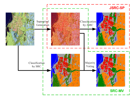
To overcome the problems of the rigid square neighborhood and high computational complexity, we propose to take advantage of contextual information in sparse representation-based PolSAR image classification by using superpixels. The concept of superpixel comes from the field of computer vision [46]. It refers to small homogenous image patches that can be considered as pure elements for classification. Using superpixels has been popular for scene classification in computer vision [47–49]. For remotely sensed image classification, using superpixels has also drawn much attention [50–53]. In this paper, we first propose a modification of the simple linear iterative clustering (SLIC) method [54] for superpixel generation in PolSAR images. The SLIC method is chosen, because it produces high quality superpixels and is simple to implement. As the original SLIC method is developed for grayscale/color images, it is modified to deal with PolSAR images by using a statistical model-based distance function. After superpixels have been obtained, they are used to define adaptive neighborhoods for incorporating contextual information within the sparse representation-based classification framework. The first strategy is to impose a spatial regularization on the pixel-wise classification map obtained by SRC. The second strategy is to take advantage of a joint sparsity model for pixels within the same superpixel. The advantage of using superpixels is two-fold. On the one hand, superpixels provide an adaptive neighborhood for each pixel; thus, the problem of including pixels from different classes when using a rigid square local window can be avoided. On the other hand, the computational burden can be effectively reduced. Experimental results with real PolSAR datasets validate the effectiveness of the proposed approaches.

The rest of the paper is organized as follows. Section 2 describes the approach of using SRC for PolSAR image classification. In Section 3, the contextual information is included for performing polarimetric-contextual classification of PolSAR images. Experimental results are presented in Section 4, and lastly, conclusions and future works are given in Section 5.

2. PolSAR Image Classification with SRC

This section presents the approach for the pixel-wise classification of PolSAR images with SRC, which consists of two ingredients: polarimetric feature extraction and sparse classification.

2.1. Polarimetric Feature Extraction

For remotely sensed image classification, informative features should be extracted to distinguish pixels of different land cover types. As mentioned in the Introduction, in this paper, the feature space for PolSAR image classification is constructed by stacking a variety of polarimetric signatures.

The ground information of PolSAR images is contained in the polarimetric measurements, i.e., scattering matrices or covariance/coherency matrices. To extract features from the measured PolSAR data, simple mathematical operations, such as absolution, summation, difference and ratio, can be used. Examples of this category of polarimetric signatures are single-channel backscattering intensities, intensity ratios, correlation coefficients, degree of polarization, etc. [55]. Although being simple to compute, those parameters are often computed with partial polarimetric measurements and, thus, can only describe a specific aspect of the ground object scattering property. We can also extract polarimetric scattering parameters with various polarimetric target decomposition methods [9]. In past decades, many polarimetric target decomposition methods have been proposed, aiming to identify ground scattering mechanisms through matrix decomposition techniques. A review of target decomposition methods is available in [1]. Generally, different target decomposition methods try to interpret PolSAR data from different perspectives. Nevertheless, there is no guidance to decide which target decomposition method will lead to the most accurate classification result for a given PolSAR image.

For a specific type of polarimetric feature extraction method, the number of extracted signatures is often small. Therefore, only partial polarimetric information is preserved. To construct a feature space with comprehensive polarimetric information, various polarimetric signatures can be stacked to form a high-dimensional feature vector at each pixel. In this paper, 42 polarimetric features are extracted from the original PolSAR data [29]. Features extracted with simple mathematical operations include the backscattering coefficients of different polarization channels, three polarized ratios, three backscattering coefficient ratios, one phase difference, the depolarization ratio and the degree of polarization. Features extracted with target decomposition methods include three parameters of the Pauli decomposition, six parameters of the Krogager decomposition, six parameters of the Cloude decomposition, six parameters of the Freeman–Durden decomposition and nine parameters of the Huynen decomposition. Although the dimensionality of such a feature space is larger than the freedom degree of the original data (six for the scattering matrix and nine for the covariance/coherency matrix in the mono-static case), it is still reasonable to construct such a redundant high-dimensional feature space, since it is difficult to design a compact optimal feature space directly. Then, the effective discriminative information contained in the redundant representation is exploited with sparse representation-based classifiers.

2.2. Sparse Representation-Based Classification of PolSAR Images

Sparse representation has been established as a powerful tool in the pattern recognition field. Wright et al. [33] proposed the SRC in the context of face recognition. The underlying assumption of SRC is that each test sample can be represented by a linear combination of a few atoms from an overcomplete dictionary. Since many atoms are not used for representing the test sample, the coefficients corresponding to those un-used atoms are zeros, leading the coefficient vector to be sparse. Let F={f₁,f₂,…,f_N}∈ℝ ^N×M be the representation of the PolSAR image in the feature space, where f_k, 1≤k≤N is the feature vector of the k-th pixel, N is the number of all pixels and M is the dimensionality of the feature space. Suppose that a training dictionary is available, which is denoted by D={d₁,d₂,…,d_NT} ∈ ℝ^N_T×M, with N_T samples and C distinct classes. In this paper, the dictionary is constructed by collecting feature samples of labeled pixels in the PolSAR image of interest. The dictionary can be arranged in a form as D=[D₁,D₂,…,D_C], in which ${\mathbf{D}}_c\in {ℝ}^{N_T^c\times M}$ is the sub-dictionary of the c-th class with $N_T^c$ samples. Therefore, we have $N_T={\sum }_{c=1}^C{N}_T^c$. It is assumed that a test polarimetric feature sample f_k can be represented with the given dictionary as follows [33]:

$$\begin{array}{l}{\mathbf{f}}_k\approx {\mathbf{d}}_1{w}_1+{\mathbf{d}}_2{w}_2+\cdots +{\mathbf{d}}_{N_T}{w}_{N_T}\\ \hspace{0.17em}\hspace{0.17em}\hspace{0.17em}=[{\mathbf{d}}_1\hspace{0.17em}{\mathbf{d}}_2\cdots \hspace{0.17em}{\mathbf{d}}_{N_T}]{[w_1\hspace{0.17em}{w}_2\hspace{0.17em}\cdots \hspace{0.17em}{w}_{N_T}]}^T=\mathbf{Dw}\end{array}$$

(1)

In Equation (1), $\mathbf{w}=\left[{\mathbf{w}}_1^T,{\mathbf{w}}_2^T,\dots ,{\mathbf{w}}_C^T\right]\in {ℝ}^{N_T\times 1}$ is the sparse combination weight vector, in which ${\mathbf{w}}_c^T\in {\text{R}}^{N_T^c\times 1}$ contains the weights corresponding to atoms of the c-th class. The key observation of SRC is that if the test sample f_k comes from the c-th class, then it can be well approximated by atoms from the same class. Therefore, the principle of SRC is to find the optimal weight vector in Equation (1) and assign the test sample to the class with the minimum approximation error.

To obtain the sparse representation of the test sample f_k, the sparse weight vector w that satisfies (1) should be solved. This leads to the following optimization problem:

$${\mathbf{w}}^{*}=\text{arg}\underset{\mathbf{w}}{\text{min}}{\Vert \mathbf{w}\Vert }_0\hspace{0.17em}\hspace{0.17em}\hspace{0.17em}\hspace{0.17em}\hspace{0.17em}s.t.\hspace{0.17em}\hspace{0.17em}\hspace{0.17em}\mathbf{Dw}\approx {\mathbf{f}}_k$$

(2)

where the l₀-norm ‖ · ‖₀ counts the non-zero elements in w. By solving the above optimization problem, we will find a weight vector with a minimum number of non-zero elements, while ensuring that the test sample is approximately represented by atoms from the dictionary. In Equation (2), the rough constraint Dw ≈ f_k is used instead of an exact constraint, so that the influence of noise and model errors can be accounted for. The problem of Equation (2) can be made more precise by using a clear requirement on the approximation accuracy, i.e., to set a bound on the approximation error. As a result, the optimization problem in Equation (2) becomes:

$${\mathbf{w}}^{*}=\text{arg}\hspace{0.17em}\hspace{0.17em}\underset{\mathbf{w}}{\text{min}}{\Vert \mathbf{w}\Vert }_0\hspace{0.17em}\hspace{0.17em}\hspace{0.17em}\hspace{0.17em}\hspace{0.17em}s.t.\hspace{0.17em}\hspace{0.17em}\hspace{0.17em}{\Vert \mathbf{Dw}-{\mathbf{f}}_k\Vert }_2\le \epsilon$$

(3)

where ɛ is the bound of the approximation error. Although the l₀ optimization problem is NP-hard, it can be approximately solved with greedy algorithms, such as orthogonal matching pursuit (OMP) [56]. To facilitate numerical computation, it is proposed to replace the l₀-norm with the l₁-norm. It is shown that if the solution of Equation (3) is sparse enough and the dictionary D is incoherent with the basis under which the solution is sparse, it can be recovered by solving the following l₁-minimization problem, as well [57,58]:

$${\mathbf{w}}^{*}=\text{arg}\hspace{0.17em}\hspace{0.17em}\underset{\mathbf{w}}{\text{min}}{\Vert \mathbf{w}\Vert }_1\hspace{0.17em}\hspace{0.17em}\hspace{0.17em}\hspace{0.17em}\hspace{0.17em}s.t.\hspace{0.17em}\hspace{0.17em}\hspace{0.17em}{\Vert \mathbf{Dw}-{\mathbf{f}}_k\Vert }_2\le \epsilon$$

(4)

The sparsity encouraging property of the l₁-norm has been studied in the field of compressive sensing. The problem in Equation (4) is known as the basis pursuit denoising (BPDN) [59]. Another equitant formulation of Equation (4) is given by the following unconstraint problem with scalar parameter ξ:

$${\mathbf{w}}^{*}=\text{arg}\hspace{0.17em}\hspace{0.17em}\underset{\mathbf{w}}{\text{min}}\frac{1}{2}\hspace{0.17em}{\Vert \mathbf{Dw}-{\mathbf{f}}_k\Vert }_2+\xi {\Vert \mathbf{w}\Vert }_1\hspace{0.17em}$$

(5)

The problem in Equations (4) and (5) are convex and, thus, can be solved efficiently with l₁-minimization techniques, such as interior point methods, proximal point methods and augmented Lagrangian methods [60]. After the sparse weight vector w is obtained, the class label for the test sample f_k is selected by:

$$l\left({\mathbf{f}}_k\right)=\text{arg}\hspace{0.17em}\hspace{0.17em}\underset{c\in \{1,2,\dots ,C\}}{\text{min}}{r}_c\left({\mathbf{f}}_k\right)$$

(6)

where r_c(f_k) = ‖f_k-D_cw_c‖₂ is the approximation error of the c-th class, l(f_k) is the label of the pixel k.

3. Polarimetric-Contextual Classification of PolSAR Images

Previous works have shown that including contextual information in the classification process helps to improve the classification performance [38–43]. For sparse representation with contextual information for remotely sensed image classification, the reader is referred to [44,45]. Although the methods in [44] can take advantage of contextual information, the considered neighborhood of a pixel is a rigid square, which may contain pixels from different classes. The method in [45] tackles this problem by assigning non-local weights to neighboring pixels. Nevertheless, this method is computational expensive, as additional non-local weights need to be computed. In this paper, we investigate alternative ways to exploit contextual information with the framework of SRC for PolSAR image classification. We combine SRC with the concept of superpixels. Based on superpixels, two strategies are considered to perform polarimetric-contextual classification of PolSAR images. Next, the method to generate superpixels in PolSAR images is first presented. Then, the methods for classification are described.

3.1. Superpixel Generation in PolSAR Images

The concept of superpixels is introduced in [46] and refers to small homogenous regions in images. Superpixels are often obtained by some over-segmentation methods. When used for classification, pixels within one superpixel are assumed to belong to the same class. In the remote sensing community, a similar concept is the so-called object-oriented analysis [50], in which over-segmented small regions (objects) are taken as analysis elements for classification. Due to the possibility of using superpixels to suppress the influence of speckle noise and clutters, a number of works have investigated superpixel-based classification of SAR/PolSAR images [51–53].

To use superpixels for PolSAR image classification, they should be generated first. Several superpixel algorithms can be found in the literature, but none is proposed for PolSAR images. The watershed algorithm [61] and normalized cut algorithm [62] have been used for superpixel generation for PolSAR images. However, the watershed algorithm produces highly irregular superpixels, and a normalized cut algorithm is computational extensive [54]. In this paper, we introduced a modified version of the SLIC algorithm [54]. Although being simple, SLIC is proven to be very effective and efficient for superpixel generation.

The basic idea of SLIC is iteratively assigning pixels to the nearest superpixels. At the beginning of the algorithm, superpixels are initialized by placing a set of seeds on the image domain. Then, the algorithm is implemented with two alternating steps: (1) fix superpixel centers and assign each pixel to the nearest superpixel according to a distance measure; (2) update superpixel centers. It should be noted that for each superpixel, only pixels in the neighborhood of the center are allowed to be assign to it. The size of the neighborhood is predefined and decides the maximum size of one superpixel.

The key issue of SLIC is the definition of the distance measure between pixels and superpixel centers. In [54], for a pixel i and a superpixel center j, the distance measure is defined as:

$$D_{\mathit{SLIC}}(i,j)=\sqrt{d_c^2(i,j)+\left(\frac{d_s(i,j)}{S}\right){\eta }^2}$$

(7)

In Equation (7), the distance between a pixel and a superpixel center is computed by combining two distances. The term d_c(i, j)=‖ c_i − c_j ‖₂ is the Euclidean distance between i and j in the color space, where c_i, c_j are color vectors of i and j respectively. The term d_s(i, j) = ‖ x_i – x_j ‖₂ is the spatial distance between i and j in the image domain, where x_i, x_j are spatial location vectors. S is the maximal size of a superpixel and η is the weight to tune the contributions of color similarity and spatial proximity.

To extend the SLIC algorithm to deal with PolSAR data, the distance measure should be modified according to the property of PolSAR data. We keep the definition of spatial distance unchanged and replace the feature-based distance with a statistical model-based measure. Statistical model-based distance measures have been proven to be more suitable than Euclidean distance for SAR/PolSAR data. In this paper, a Wishart distribution-based distance d_s(i, j) is used [10]:

$$d_p(i,j)=\text{ln}\left(\left|{\mathbf{\Sigma }}_j\right|\right)+\text{Tr}\left({\mathbf{\Sigma }}_j^{-1}{\mathbf{T}}_i\right)$$

(8)

where T_i is the coherency matrix of pixel i and Σ_j is the mean coherency matrix of the superpixel centered at j. Substituting d_p(i, j) into Equation (7) to replace the color-based distance d_c(i, j) gives the distance measure for superpixel generation for PolSAR images.

After superpixels have been generated, we have a collection of superpixels {sp_j, j=1,…,N_sp}, where N_sp is the number of all superpixels. For each superpixel, pixels within it are assumed to belong to the same class. The next step is to incorporate contextual information derived from the superpixel map into sparse representation-based classification. In this paper, two approaches have been considered to combine polarimetric and contextual information together.

3.2. Combining SRC with Superpixels by Majority Voting

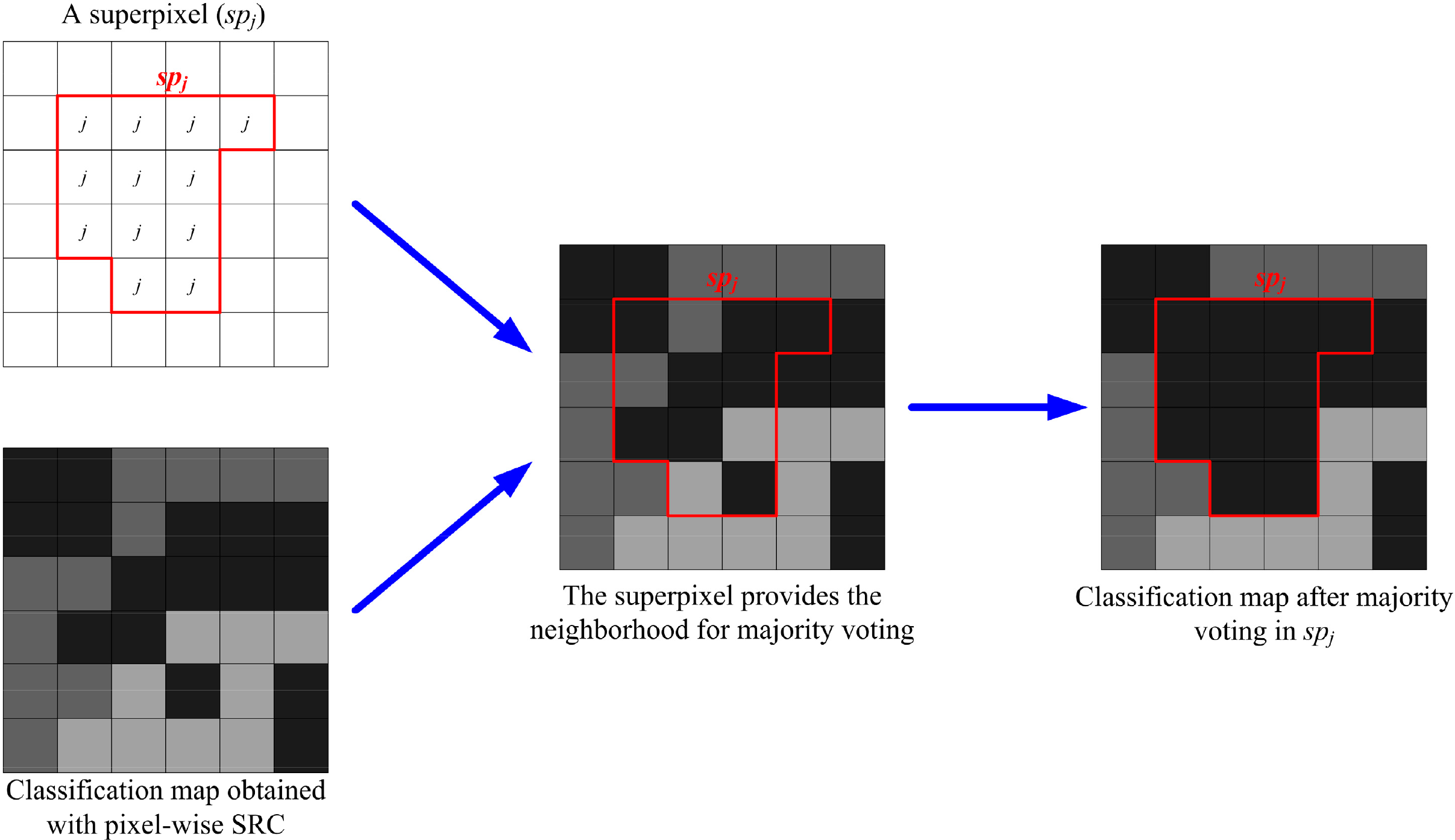
The first approach that has been considered is to regularize the pixel-wise classification map obtained with SRC by superpixel-based majority voting. Majority voting is a long-standing and popular method for combing the results of a set of classifiers. It has been considered to improve the classification result obtained by SVM for hyperspectral images [63]. Note that the majority voting with rigid neighborhoods can also impose spatial regularization on pixel-wise classification maps. However, using an adaptive neighborhood, such as superpixel (or segments in [63]), helps to preserve class boundaries and suppress over-smoothness. In our case, each superpixel in the PolSAR image is taken as a unit, and pixels in it are all supposed to have the same class label. However, the pixel-wise SRC classifies each pixel independently. This can be considered as classifying a superpixel with different descriptors (i.e., feature vectors associated with pixels in the superpixel). Therefore, the majority voting is actually a decision fusion process, in which the classification results with different descriptors are combined together.

The principle of superpixel-based majority voting is shown in Figure 1. For a given superpixel, we count the times that each class label presents in that superpixel. The class label that presents most often is selected and assigned to all pixels within that superpixel. The decision rule of majority voting is formally defined as:

$$l({\mathit{sp}}_j)=\text{arg}\underset{c\in \{1,2,\dots ,C\}}{\text{max}}\left[\sum _{i\in {\mathit{sp}}_j}\delta \left(l(i)-c\right)\right]$$

(9)

where δ(z) is the Dirac function, sp_j denotes the superpixel index by j and l(sp_j), l(i) denote the label of superpixel sp_j and pixel i, respectively.

3.3. Polarimetric-Contextual Classification with Superpixel-Based JSRC

Another strategy to combine polarimetric and contextual information is to classify each superpixel directly according to the features within it. One way is to compute a single descriptor for each superpixel, e.g., the mean feature vector, and then classify it with the produced single descriptor. However, this may cause information loss. Nevertheless, in the framework of sparse representation-based classification, this problem can be addressed with a joint sparsity model [64,65]. The underlying assumption of the joint sparsity model is that if a set of test samples are from the same class, they can be represented by similar dictionary atoms (i.e., the associated sparse representation weight vectors share the similar sparsity pattern). It is shown that by making use of the correlation between weight vectors, a more accurate sparse model can be derived. In our case, since pixels within one superpixel are considered to belong to the same class, the corresponding feature vectors would share a similar sparsity pattern. Therefore, we can solve the sparse representation weight vectors for all pixels in a superpixel simultaneously with a constraint that forces those weight vectors to have similar non-zero elements.

Consider a specific superpixel sp_j in the PolSAR image, which contains N_j pixels associated with the same number of polarimetric feature vectors. Those feature vectors are arranged in a matrix as:

$${\mathbf{F}}_j=\left[{\mathbf{f}}_1^j,{\mathbf{f}}_2^j,\cdots ,{\mathbf{f}}_{N_j}^j\right]$$

(10)

Each feature vector of sp_j can be represented by the dictionary D as ${\mathbf{f}}_k^j\approx \mathbf{D}{\mathbf{w}}_k^j$, ∀1≤k≤N_j. Collecting all weight vectors in a matrix, we have ${\mathbf{W}}_j=\left[{\mathbf{w}}_1^j,{\mathbf{w}}_2^j,\dots ,{\mathbf{w}}_{{\text{N}}_{\text{j}}}^j\right]$. As a result, F_j can be represented by:

$$\begin{array}{l}{\mathbf{F}}_j=\left[{\mathbf{f}}_1^j,{\mathbf{f}}_2^j,\cdots ,{\mathbf{f}}_{N_j}^j\right]\approx \left[\mathbf{D}{\mathbf{w}}_1^j,\mathbf{D}{\mathbf{w}}_2^j,\cdots \mathbf{D}{\mathbf{w}}_{N_j}^j\right]\\ \hspace{0.17em}\hspace{0.17em}\hspace{0.17em}\hspace{0.17em}=\mathbf{D}[{\mathbf{w}}_1^j,{\mathbf{w}}_2^j,\cdots ,{\mathbf{w}}_{N_j}^j]=\mathbf{D}{\mathbf{W}}_j\end{array}$$

(11)

In the joint sparsity model, the weight matrix W_j should satisfy two requirements: (1) each column is sparse; (2) the non-zero elements in all columns should be located at similar positions. It turns out that such constraints can be forced by minimizing the row-l₀ norm ‖W_j‖_row,0, which counts the non-zero rows of W_j [66]. Therefore, the optimization problem associated with the joint sparse model is:

$${\mathbf{W}}_j^{*}=\text{arg}\hspace{0.17em}\hspace{0.17em}\underset{{\mathbf{W}}_j}{\text{min}}{\Vert {\mathbf{W}}_j\Vert }_{\mathit{row},0}\hspace{0.17em}\hspace{0.17em}\hspace{0.17em}s.t.\hspace{0.17em}\hspace{0.17em}\hspace{0.17em}{\mathbf{F}}_j\approx \mathbf{D}{\mathbf{W}}_j$$

(12)

Similar to the derivation of Equation (3), the model in Equation (12) can also be made more precise by introducing an error bound:

$${\mathbf{W}}_j^{*}=\text{arg}\hspace{0.17em}\hspace{0.17em}\underset{{\mathbf{W}}_j}{\text{min}}{\Vert {\mathbf{W}}_j\Vert }_{\mathit{row},0}\hspace{0.17em}\hspace{0.17em}\hspace{0.17em}s.t.\hspace{0.17em}\hspace{0.17em}\hspace{0.17em}{\Vert {\mathbf{F}}_j-{\mathbf{DW}}_j\Vert }_F\le \epsilon$$

(13)

Where ‖ · ‖_F denotes the Frobenius norm and ɛ is the bound of the approximation error.

Minimizing Problem (13) is difficult, just like the situation for the sparse representation of a single signal. This problem is often addressed by relaxing the problem by replacing the row-l₀ norm with a more tractable norm [66]. In this paper, we use the l₁ − l₂ norm, which is defined as:

$${\Vert {\mathbf{W}}_j\Vert }_{1,2}=\sum _{n=1}^{N_T}\sqrt{\sum _{k=1}^{N_j}{(w_{n,k}^j)}^2}$$

(14)

where $w_{n,k}^j$ denotes the elements of W_j at row n and column k.

Replacing the row-l₀ norm in Equation (14) with the l₁ − l₂ norm yields the following optimization problem:

$${\mathbf{W}}_j^{*}=\text{arg}\hspace{0.17em}\hspace{0.17em}\underset{{\mathbf{W}}_j}{\text{min}}\Vert {\mathbf{W}}_j{\Vert }_{1,2}\hspace{0.17em}\hspace{0.17em}\hspace{0.17em}s.t.\hspace{0.17em}\hspace{0.17em}\hspace{0.17em}\Vert {\mathbf{F}}_j-\mathbf{D}{\mathbf{W}}_j{\Vert }_F\le \epsilon$$

(15)

or equivalently:

$${\mathbf{W}}_j^{*}=\text{arg}\hspace{0.17em}\hspace{0.17em}\underset{{\mathbf{W}}_j}{\text{min}}\Vert {\mathbf{F}}_j-\mathbf{D}{\mathbf{W}}_j{\Vert }_F+\xi \Vert {\mathbf{W}}_j{\Vert }_{1,2}$$

(16)

Solving Equation (15) or Equation (16) gives the weight matrix ${\mathbf{W}}_j^{*}={\left[{\left({\mathbf{W}}_{j,1}^{*}\right)}^T,{\left({\mathbf{W}}_{j,2}^{*}\right)}^T,\dots ,{\left({\mathbf{W}}_{j,C}^{*}\right)}^T\right]}^T$, in which the matrix ${\mathbf{W}}_{k,c}^{*}$ represents the weights to represent F_j with training samples in the c-th class. Now, the reconstruction error of the c-th class for the superpixel sp_j can be computed by:

$$r_{j,c}\left({\mathbf{F}}_j\right)=\Vert {\mathbf{D}}_c{\mathbf{W}}_{j,c}^{*}-{\mathbf{F}}_j{\Vert }_F$$

(17)

The class label for pixels in the superpixel sp_j is given by:

$$l\left({\mathit{sp}}_j\right)=\text{arg}\hspace{0.17em}\hspace{0.17em}\underset{c\in \{1,2,\dots ,C\}}{\text{min}}{r}_{j,c}\left({\mathbf{F}}_j\right)$$

(18)

It should be noted that although the proposed approach and the approaches in [44,45] are all based on the JSRC, they are quite different. In the methods of [44,45], the classification is performed pixel-wise. At each pixel, the associated feature vector and feature vectors of neighboring pixels are sparsely represented simultaneously to classify that pixel. Therefore, the number of processing elements is the same as the number of pixels. On the contrary, in the proposed approach, we have obtained the superpixel map, and the classification is performed at the superpixel level. As a result, the number of processing elements is the same as the number of superpixels, which is much less than the number of pixels. This will help to reduce the computational burden. Moreover, the neighborhoods of the method in [44] are rigid squares; thus, they may include pixels of different classes. Although the method in [45] addresses this problem by using non-local weights, the computational complexity is further increased. In contrast, the neighborhoods are adaptively selected by superpixels in the proposed approach, thus avoiding the problem caused by rigid neighborhoods.

4. Results and Discussion

In this section, we evaluate the effectiveness of the proposed sparse representation- and superpixel-based PolSAR image classification approaches. The main objective of the experimental validation is two-fold. Firstly, the ability of sparse representation-based classifiers to produce favorable PolSAR image classification is verified. To achieve this, the proposed approach is compared with the widely-used Wishart model-based classifiers. Since the proposed two approaches exploit contextual information, two Wishart model-based competitors, which also make use of contextual information, are considered. One is a region-based Wishart maximum-likelihood (Wishart-ML) classifier [10], which takes superpixels as processing elements [53]. The other one is the Wishart-MRF classifier [14,15], which exploits contextual information by using the MRF model. We adopt the well-known graph cut algorithm [67] for energy optimization for the sake of efficiency. In addition, the SVM-based on composite kernel (SVMCK) classifier [68] is also tested. The SVM-based classifiers are shown to be powerful tools in the remote sensing field and have been successfully applied on PolSAR images [27,29]. Using composite kernels enables us to incorporate contextual information into the SVM classifier. The second objective of the experimental validation is to demonstrate the advantage of combining sparse representation-based classifiers with superpixels. This is achieved by comparing the proposed two approaches with other sparse representation-based classifiers. The results obtained by the pixel-wise SRC approach are presented to show the gain on classification accuracy by making use of contextual information. Moreover, two joint sparse representation-based classifiers are also evaluated, which are the joint sparse representation-based approach that considered square neighborhoods (JSRC-SQ) [44] and the improved approach with non-local weights (JSRC-NLW) [45]. The approaches proposed in this paper are denoted as SRC-MV and JSRC-SP, respectively. It should be noted that all approaches make use of the same polarimetric features, except the two Wishart model-based classifiers.

In practice, we can solve Equation (3) or Equation (5) to implement SRC, as well as Equation (13) or Equation (16) to implement JSRC. Nevertheless, in this paper, we do not intend to evaluate and compare the advantages and disadvantages of using different sparsity-promoting norms. Therefore, in all experiments, Problem (3) is adopted for SRC and is solved with the OMP algorithm. For JSRC, Problem (16) is adopted and is solved by the simultaneous OMP (SOMP) algorithm. The approximation error bound is set as 0.001 for SRC and 0.01 for JSRC. As can be observed in the following experiments, although being suboptimal, this setting provides very good classification results. Following the work of [68], the spatial kernel in the SVMCK approach is constructed by using the mean feature vector of a 5 × 5 local window centered at each pixel. Besides, the SVM parameters are decided by five-fold cross-validation. The weight for kernel summation is varied in the range [0, 1] with steps of 0.1. The penalizing factor in the SVM is tuned in the range of {10⁻², 10⁻¹_, …, 10⁵}. The radial basis function kernel is used with the width parameter ranges in{10⁻², 10⁻¹_, …, 10³}. The neighborhood size of JSRC-SQ and JSRC-NLW is chosen between 3 × 3 and 13 × 13 according to [44,45]. For the proposed two approaches and the Wishart-ML approach, the sizes of superpixels are varied. Nevertheless, we initialize the superpixel seeds as regular patches with a fixed size, so that the mean superpixel size can be roughly controlled (as the number of superpixels is decided by the initial patch size). The weight parameter η in Equation (7) is set as two, which empirically keeps a reasonable balance between the compactness and feature coherence of superpixels. All of the experiments were conducted using MATLAB R2010b on a 3.40-GHz machine with 4.0 GB RAM.

We evaluate different algorithms on two different real PolSAR datasets. In our experiments, the training samples are randomly selected from the available reference data and the remaining samples are used for validation purposes. This strategy is widely admitted in the remote sensing community [39,40]. In the case that a superpixel contains training samples, the selected pixels are excluded from the superpixel in the classification process. The same disposition is used when the neighborhood of a pixel contains training samples for JSRC-SQ and JSRC-NLW. The overall accuracy (OA) and kappa coefficient are used to evaluate the accuracy performance of the classification. The efficiency of different algorithms is assessed by the CPU time cost. The performance indexes are obtained by averaging the values obtained after ten Monte Carlo runs. Following, we report the experimental results on two real PolSAR images.

4.1. RadarSat-2 Flevoland Dataset

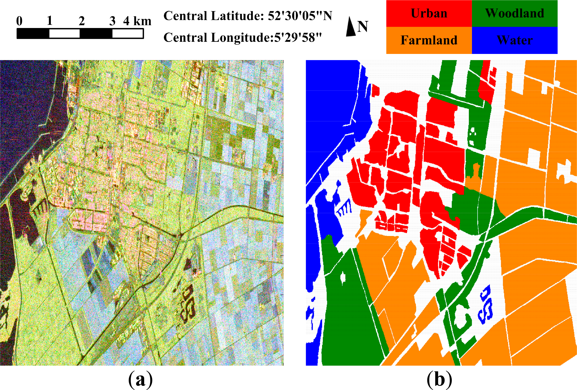
The first dataset is a C-band fully-polarimetric SAR image collected by the RadarSat-2 system at the fine quad mode over the area of Flevoland, Netherland. The used subset consists of 700 × 780 pixels. Figure 2a is a false color image obtained by Pauli decomposition, and Figure 2b is the manually-labeled reference map. A total of four classes are identified, which are the building area, woodland, farmland and water area. Pixels with no reference label are shown in gray.

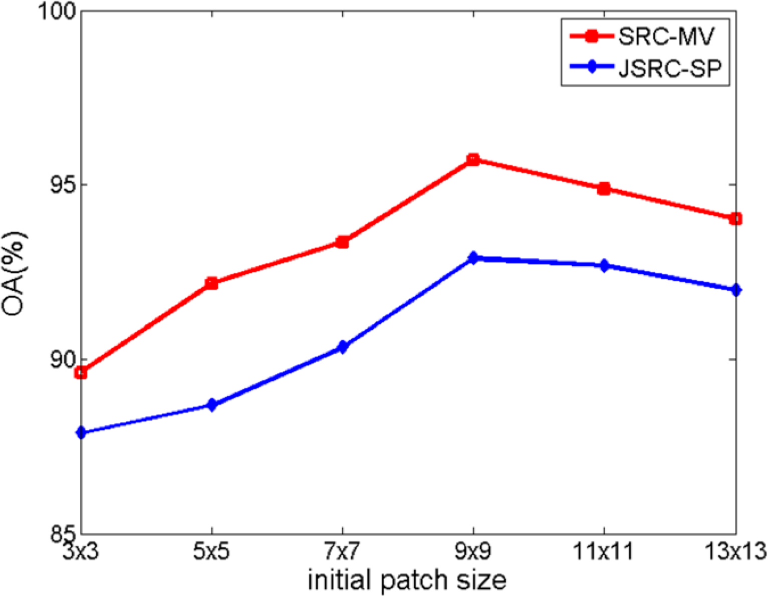
The first experiment with the RadarSat-2 dataset is to illustrate the feasibility and advantage of using superpixels to incorporate contextual information into the sparse representation-based classification framework for PolSAR images. We constructed the training dictionary by randomly selecting 1% of the available labeled pixels as atoms. In our experiment, we noticed that the size of the initial patches for superpixel generation could affect the classification accuracy. Therefore, we conducted an additional experiment to analyze the effect of initial patch size on the classification accuracy. Figure 3 shows the change of the OA when the initial patch size increases from 3 × 3 to 13 × 13. It can be noticed that the best OA occurs when the initial patch size is 9 × 9 for both approaches. For the proposed two approaches, the highest OAs reach 95.72% (SRC-MV) and 92.89% (JSRC-SP), respectively, which are both much higher that the OA of 86.02% achieved by SRC. This demonstrates the effectiveness of using superpixels for incorporating contextual information for sparse representation-based PolSAR image classification. Besides, we can also conclude that the size of superpixels could have an impact on the classification accuracy.

To further validate the performance of the proposed two approaches, we report results obtained by other competitors. Figure 4 shows the classification obtained by different approaches by using 1% of labeled pixels as training samples. In Figure 4a, the superpixels generated with 9 × 9 initial patches are illustrated. This superpixel map is then used in the proposed SRC-MV approach and JSRC-SP approach, as well as the Wishart-ML approach. The optimal neighborhood size for the JSRC-SQ approach and JSRC-NLW approach are 7 × 7 and 11 × 11, respectively. Several observations can be made from Figure 4. Firstly, compared with other approaches, SRC produces the most noisy classification result, notably in the woodland and building areas, which have strong textures. This proves the importance of taking advantage of contextual information for the classification of PolSAR images. Secondly, the two Wishart model-based approaches have relatively poor performance. When the resolution of the PolSAR image increases and the texture is present in the image, the scene becomes heterogeneous and the applicability of the Wishart model reduces. As a result, classification with the Wishart model may have limited accuracy. Finally, it should be noticed that for superpixel-based approaches, a superpixel is considered as a whole for classification. Therefore, if a wrong classification decision is made, then all pixels in a superpixel may be forced to have the wrong class label. This phenomenon can be observed from Figure 4c,d,h.

In

Table 1. Classification accuracy measures on the Flevoland dataset. The best performance in each column is shown in bold. SVMCK, SVM-based on composite kernel.

Method	Building	Woodland	Farmland	Water	OA	Kappa
SRC	75.47	78.22	89.79	95.77	85.66	0.792
SRC-MV	88.96	94.83	97.81	98.59	95.72	0.938
JSRC-SP	83.10	89.86	96.40	98.06	92.89	0.896
JSRC-SQ	78.91	94.11	96.56	96.40	92.88	0.896
JSRC-NLW	84.05	90.63	95.85	98.37	93.01	0.898
SVMCK	71.65	97.91	86.62	99.11	88.22	0.832
Wishart-ML	64.65	96.87	79.37	96.04	82.94	0.759
Wishart-MRF	63.63	96.46	80.16	98.49	83.41	0.767

, we report the quantitative accuracy indexes for different approaches on the RadarSat-2 dataset. From Table 1, we can notice the poor performance of Wishart model-based approaches. Even though the contextual information has been exploited, the classification accuracy is still less than the pixel-wise SRC approach. This clearly demonstrates the advantage of collecting varies polarimetric signatures to unfold the discriminative information contained in PolSAR data. However, the pixel-wise SRC approach still has relatively low classification accuracy compared with other polarimetric-contextual approaches. Among those approaches, sparse representation-based approaches provide favorable performance. The proposed JSRC-SP approach produces accuracy indexes that are very close to those obtained by JSRC-SQ and that are a bit lower than those obtained by JSRC-NLW. The advantage of the proposed JSRC-SP approach is that it can choose adaptive neighborhoods for classification and avoids the neighborhoods containing pixels from different classes. However, as the reference map is non-exhaustive, few labeled pixels are located at terrain class boundaries. Therefore, we would expect that the JSRC-SQ approach will achieve similar accuracy performance as the JSRC-SP approach. Nevertheless, the SRC-MV approach reaches the highest OA and kappa coefficient among all of the approaches.

Another important aspect to assess the performance of algorithms is the efficiency. In

Table 2. The running processing time of different methods on the Flevoland dataset in seconds.

Methods	SRC	SRC-MV	JSRC-SP	JSRC-SQ	JSRC-NLW	SVMCK
Time (s)	261.57	303.45	112.83	7659.88	8577.88	137.43

, we report the running times for different approaches. We only present the running time for polarimetric feature vector-based approaches, since those two Wishart model-based approaches have relatively poor accuracy performance. For the remaining six approaches, the time for feature extraction is not counted, since it is the same for all approaches. Besides, for superpixel-based approaches, the time for superpixel generation is added to the overall running time. It can be seen that both the JSRC-SQ approach and the JSRC-NLW approach have a rather long time cost compared with other approaches. This is because both approaches need to solve a joint sparse representation problem at each pixel. On the other hand, the proposed two approaches take much less time to produce the final classification result. The JSRC-SP is the most efficient approach among those six approaches. The reason is that in JSRC-SQ, the classification is performed at the superpixel level, thus the number of processing units is much less than the number of pixels in the image. This helps to save a lot time. The SRC-MV approach has a relatively low efficiency compared with JSRC-SP. Nevertheless, in this study case, it produces higher accuracy performance.

4.2. EMISAR Foulum Dataset

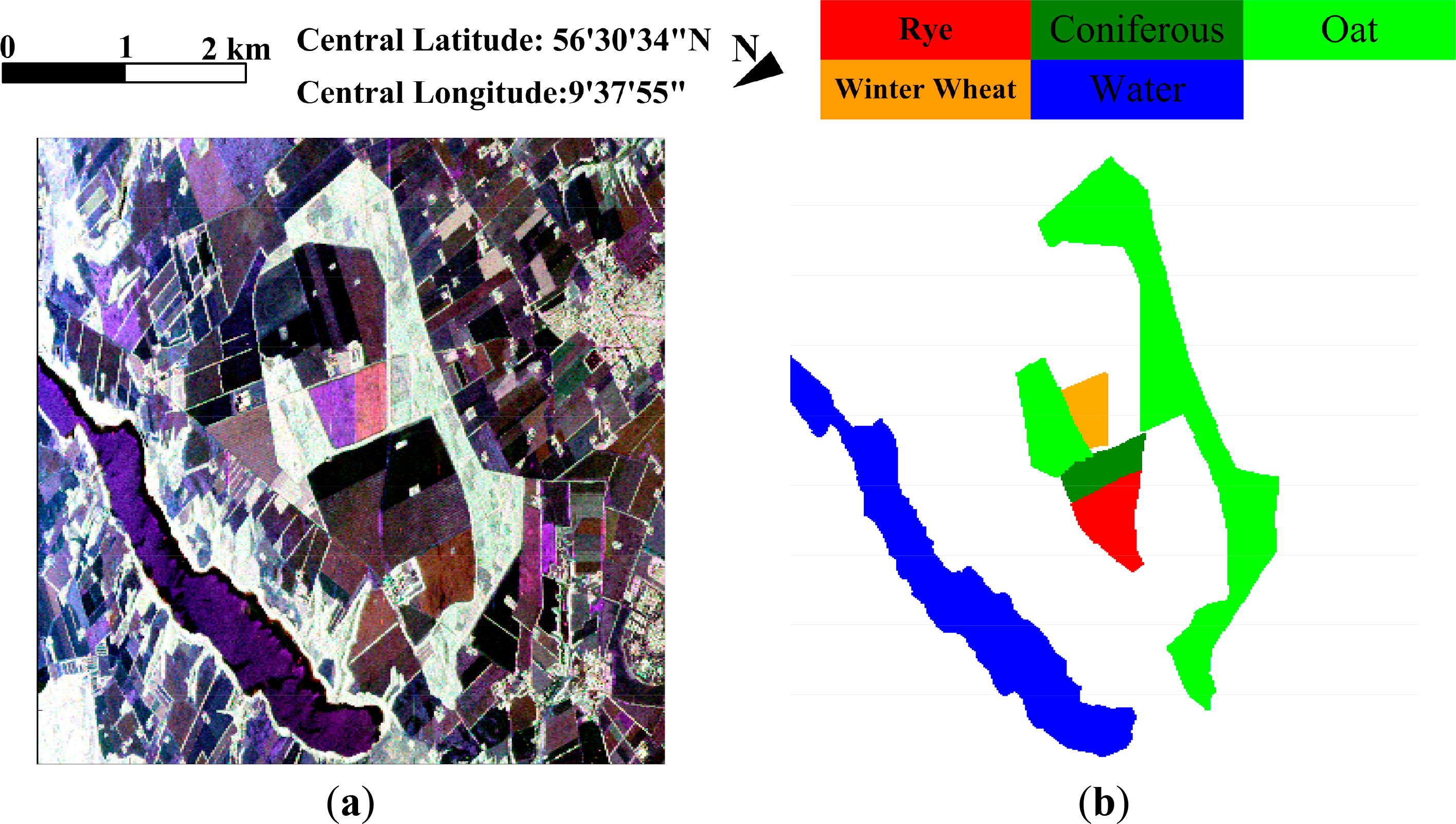
This scene was acquired by the C-band fully-polarimetric EMISAR system in April, 1998, over the area of Foulum, Denmark. In Figure 5a, the 332 × 437-pixel false color image obtained by Pauli decomposition is illustrated. A reference map with five classes has been created [30], as shown in Figure 5b. The five classes are rye, coniferous, oat, winter wheat and water. Unlabeled pixels are shown in gray. This scene constitutes a challenging classification problem due to the highly intra-class heterogeneity and because of the unbalanced number of available labeled pixels per class. We randomly sampled 5% of the labeled pixels for each class as training samples, and the rest of the labeled pixels are taken as test samples.

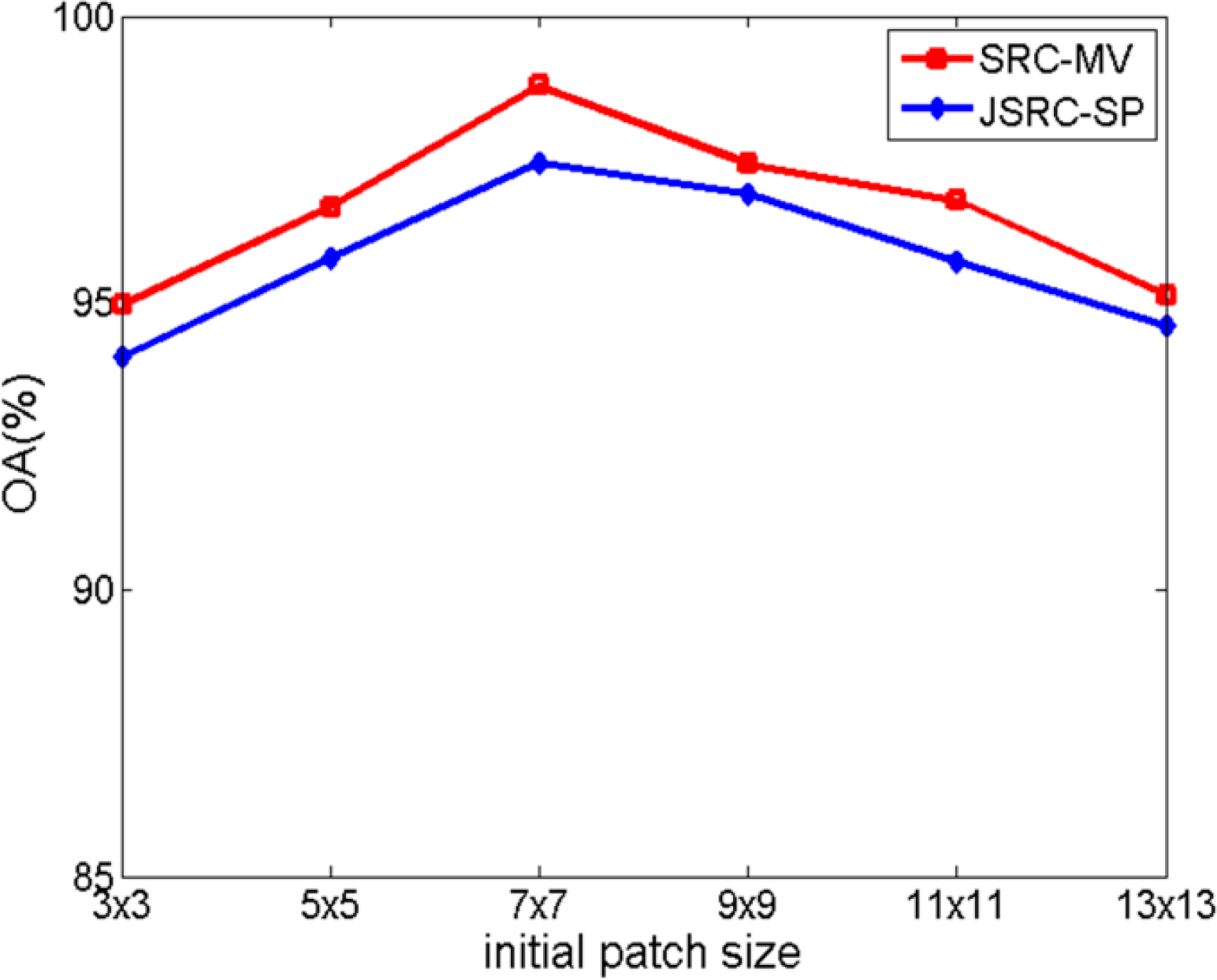
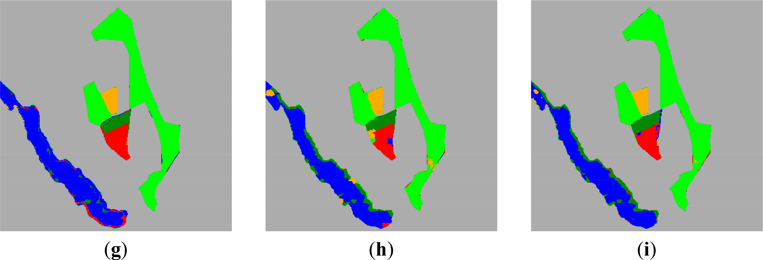
Similar to the processing of the first dataset, we conducted an experiment to decide the optimal initial patch size for superpixel generation. We find that the best accuracy performance is reached when the initial patch size is 7 × 7 (as shown in Figure 6). In Figure 7a, the generated superpixels are illustrated. The optimal neighborhood sizes for the JSRC-SQ approach and JSRC-NLW approach are 7 × 7 and 9 × 9, respectively. Figure 6b–i shows the classification result obtained by different approaches. It can be observed that while the SRC approach produces much noise, like errors, the Wishart model-based approaches cause many errors for the water class due to the strong heterogeneity of the scattering mechanism. For the other approaches, evaluating the classification performance by visual interpretation is difficult. Therefore, we computed quantitative indexes, which are reported in

Table 3. Classification accuracy measures on the EMISAR Foulum dataset. The best performance in each column is shown in bold.

Method	Water	Rye	Coniferous	Winter Wheat	Oat	OA	Kappa
SRC	87.71	96.87	88.47	92.79	99.26	94.02	0.906
SRC-MV	98.21	99.13	96.01	97.26	99.59	98.79	0.981
JSRC-SP	96.48	95.35	96.01	93.16	98.96	97.44	0.958
JSRC-SQ	95.48	92.07	97.09	91.04	99.13	96.90	0.951
JSRC-NLW	96.35	92.51	95.15	92.79	99.66	97.49	0.960
SVMCK	92.56	87.20	81.47	88.56	98.87	94.59	0.913
Wishart-ML	76.08	84.87	89.87	93.41	97.72	88.18	0.818
Wishart-MRF	78.32	90.33	92.78	95.65	99.02	90.21	0.848

.

The running time of different approaches on the EMISAR Foulum dataset is shown in

Table 4. The running processing time of different methods on the EMISAR Foulum dataset in seconds.

Methods	SRC	SRC-MV	JSRC-SP	JSRC-SQ	JSRC-NLW	SVMCK
Time (s)	18.68	28.33	13.05	418.91	432.68	17.87

. Similar to the observation on the RadarSat-2 Flevoland dataset, a significant running time reduction has been achieved by the proposed approaches compared with JSRC-SQ and JSRC-NLW. The JSCR-SP approach is the most efficient one among the compared approaches. SRC-MV costs more time than JSRC-SP, SRC, as well as SVMCK, but produces better accuracy performance.

5. Conclusions

In this paper, we have investigated the classification of PolSAR images with sparse representation-based classifiers and have gained several achievements. We investigated the feasibility of using sparse representation-based methods for PolSAR image classification. It is shown that by using sparse representation-based classification methods, superior classification performance can be obtained for PolSAR images when compared with traditional Wishart model-based classifiers. Moreover, two novel strategies, based on majority voting and joint sparse representation with superpixels, respectively, were proposed to incorporate contextual information for sparse representation-based PolSAR image classification. It is shown that sparse representation-based PolSAR image classification can benefit from incorporating contextual information with superpixels. When compared with the pixel-wise SRC classifier, using contextual information helps to improve the classification performance. Moreover, using superpixels not only makes the contextual information adaptive, but also helps to save on computational burden. Therefore, the proposed approaches can achieve favorable classification accuracy with reduced computational burden when compared to previous joint sparse representation-based approaches for remote sensing image classification.

Comparative experiments with real PolSAR datasets have been conducted to verify the performance of the proposed approaches. Two real PolSAR images have been used: a RadarSat-2 dataset over the region of Flevoland and an EMISAR dataset over the area of Foulum. Experimental results demonstrate that the proposed approaches provide favorable classification performance when compared against the region-based Wishart-ML classifier, Wishart-MRF classifier, SVMCK classifier, pixel-wise sparse representation-based classifier and two other joint sparse representation-based classifiers. The proposed SRC-MV approach achieves the highest classification accuracy on both tested datasets (95.72% on the RadatSat-2 dataset and 98.79% on EMISAR dataset). The other approach proposed in this paper (JSRC-SP) also produces accurate classification result on both datasets. The overall accuracy is 92.89% on the RadarSat-2 dataset and 97.44% on the EMISAR dataset, which are noticeably higher than SRC, Wishart-ML, Wishart-MRF and SVMCK and are competitive compared with other two joint sparse representation-based classifiers. Further evaluation of the running time demonstrates that the proposed two approaches have favorable efficiency. Among the compared approaches, the proposed JSRC-SP is the most efficient one (112.83 s for the RadarSat-2 dataset and 13.05 s for the EMISAR dataset). Considering its high efficiency, the JSRC-SP approach could be an interesting candidate approach when efficiency is an important factor.

In consideration of the above achievements and results, we not only enrich the family of sparse representation-based classification methods by using superpixels for incorporating contextual information, but also provide interesting alternate approaches for PolSAR image classification.

Future work will be focused on improving the performance of PolSAR image classification with sparse representation techniques. One possible direction is to construct a better dictionary with dictionary learning methods. It is expected that the classification accuracy will be further enhanced by exploiting the discriminant information in the training samples when learning the dictionary. Another line is to cope with the possible non-linear property of PolSAR features with kernel methods. Other strategies to exploit contextual information will also be studied. For example, it is possible to combine SRC with smooth-promoting models, such as the MRF model or variational methods. The key issue will be how to take advantage of the outputs of SRC in those models.

References

- Touzi, R.; Boerner, W.M.; Lee, J.S.; Lueneburg, E. A review of polarimetry in the context of synthetic aperture radar: Concepts and information extraction. Can. J. Remote Sens 2004, 30, 380–407. [Google Scholar]
- Novak, L.M.; Halversen, S.D.; Owirka, G.J.; Hiett, M. Effects of polarization and resolution on SAR ATR. IEEE Trans. Aerosp. Electron. Syst 1997, 33, 102–116. [Google Scholar]
- Lee, J.S.; Grunes, M.R.; Pottier, E. Quantitative comparison of classification capability: Fully polarimetric versus dual and single-polarization SAR. IEEE Trans. Geosci. Remote Sens 2001, 39, 2343–2351. [Google Scholar]
- Cloude, S.R.; Pottier, E. An entropy based classification scheme for land applications of polarimetric SAR. IEEE Trans. Geosci. Remote Sens 1997, 35, 68–78. [Google Scholar]
- Ferro-Famil, L.; Pottier, E.; Lee, J.S. Unsupervised classification of multifrequency and fully polarimetric SAR images based on H/a/Alpha- Wishart classifier. IEEE Trans. Geosci. Remote Sens 2001, 39, 2332–2342. [Google Scholar]
- Hoekman, D.H.; Vissers, M.A.; Tran, T.N. Unsupervised full-polarimetric SAR data segmentation as a tool for classification of agricultural areas. IEEE J. Sel. Top. Appl. Earth Obs. Remote Sens 2011, 4, 402–411. [Google Scholar]
- Quegan, S.; Rhodes, I. Statistical models for polarimetric data: Consequences, testing and validity. Int. J. Remote Sens 1995, 16, 1183–1210. [Google Scholar]
- Freitas, C.C.; Frery, A.C.; Correia, A.H. The polarimetric G distribution for SAR data analysis. Environmetrics 2005, 16, 13–31. [Google Scholar]
- Cloude, S.R.; Pottier, E. A review of target decomposition theorems in radar polarimetry. IEEE Trans. Geosci. Remote Sens 1996, 34, 498–518. [Google Scholar]
- Lee, J.S.; Grunes, M.R.; Kwok, R. Classification of multi-look polarimetric SAR imagery based on complex Wishart distribution. Int. J. Remote Sens 1994, 15, 2299–2311. [Google Scholar]
- Doulgeris, A.; Anfinsen, S.; Eltoft, T. Automated non-Gaussian clustering of polarimetric synthetic aperture radar images. IEEE Trans. Geosci. Remote Sens 2011, 49, 3665–3676. [Google Scholar]
- Formont, P.; Pascal, F.; Vasile, G. Statistical classification for heterogeneous polarimetric SAR images. IEEE J. Sel. Top. Appl. Earth Obs. Remote Sens 2011, 5, 567–576. [Google Scholar]
- Conradsen, K.; Nielsen, A.; Schou, J.; Skriver, H. A test statistic in the complex Wishart distribution and its application to change detection in polarimetric SAR data. IEEE Trans. Geosci. Remote Sens 2003, 41, 4–19. [Google Scholar]
- Wu, Y.; Ji, K.; Yu, W.; Su, Y. Segmentation of multi-look fully polarimetric SAR images based on Wishart distribution and MRF. Proc. SPIE 2007, 6748, 674813:1–674813:9. [Google Scholar]
- Wu, Y.; Ji, K.; Yu, W.; Su, Y. Region-based classification of polarimetric SAR images using Wishart MRF. IEEE Geosci. Remote Sens. Lett 2008, 5, 668–672. [Google Scholar]
- Ayed, I.B.; Mitiche, A.; Belhadj, Z. Polarimetric image segmentation via maximum-likelihood approximation and efficient multiphase level-sets. IEEE Trans. Pattern Anal. Mach. Intell 2006, 28, 1493–1500. [Google Scholar]
- Gao, W.; Yang, J.; Ma, W. Land cover classification for polarimetric SAR images based on mixture models. Remote Sens 2014, 6, 3770–3790. [Google Scholar]
- Anfinsen, S.; Eltoft, T. Application of the matrix-variate Mellin transform to analysis of polarimetric radar images. IEEE Trans. Geosci. Remote Sens 2011, 49, 2281–2781. [Google Scholar]
- Anfinsen, S.; Doulgeris, A.; Eltoft, T. Goodness-of-fit tests for multilook polarimetric radar data based on the Mellin transform. IEEE Trans. Geosci. Remote Sens 2011, 49, 2764–2295. [Google Scholar]
- Van Zyl, J.J. Unsupervised classification of scattering behavior using radar polarimetry data. IEEE Trans. Geosci. Remote Sens 1989, 27, 36–45. [Google Scholar]
- Lee, J.S.; Grunes, M.R.; Pottier, E.; Ferro-Famil, L. Unsupervised terrain classification preserving polarimetric scattering characteristics. IEEE Trans. Geosci. Remote Sens 2004, 42, 722–731. [Google Scholar]
- Yonezawa, C.; Watanabe, M.; Saito, G. Polarimetric decomposition analysis of ALOS PALSAR observation data before and after a landslide event. Remote Sens 2012, 4, 2314–2328. [Google Scholar]
- Huynen, J.R. Phenomenological Theory of Radar Targets. Ph.D. Dissertation, Delft University, Delft, The Netherlands. 1970. [Google Scholar]
- Yamaguchi, Y.; Moriyama, T.; Ishido, M.; Yamada, H. Four component scattering model for polarimetric SAR image decomposition. IEEE Trans. Geosci. Remote Sens 2005, 43, 1699–1706. [Google Scholar]
- Cameron, W.L.; Youssef, N.N.; Leung, L.K. Simulated polarimetric signatures of primitive geometrical shapes. IEEE Trans. Geosci. Remote Sens 1996, 34, 793–803. [Google Scholar]
- Krogager, E. New decomposition of the radar target scattering matrix. Electron. Lett 1990, 26, 1525–1527. [Google Scholar]
- Lardeux, C.; Frison, P.L.; Tison, C.; Stoll, B.; Fruneau, B.; Rudant, J.-P. Support vector machine for multifrequency SAR polarimetric data classification. IEEE Trans. Geosci. Remote Sens 2009, 47, 4143–4152. [Google Scholar]
- Zou, T.Y.; Yang, W.; Dai, D.X.; Sun, H. Polarimetric SAR image classification using multifeatures combination and extremely randomized clustering forests. EURASIP J. Adv. Signal Process 2010, 2010, 465612:1–465612:9. [Google Scholar]
- Tu, S.T.; Chen, J.Y.; Yang, W.; Sun, H. Laplacian eigenmaps based polarimetric dimensionality reduction for SAR image classification. IEEE Trans. Geosci. Remote Sens 2012, 50, 170–179. [Google Scholar]
- Shi, L.; Zhang, L.; Yang, J. Supervised graph embedding for polarimetric SAR image classification. IEEE Geosci. Remote Sens. Lett 2013, 10, 216–220. [Google Scholar]
- Pajares, G.; López-Martínez, C.; Sánchez-Lladó, F.J.; Molina, Í. Improving Wishart classification of polarimetric SAR data using the hopfield neural network optimization approach. Remote Sens 2012, 4, 3571–3595. [Google Scholar]
- She, X.L.; Yang, J.; Zhang, W.J. The boosting algorithm with application to polarimetric SAR image classification. In Proceedings of the 1st Asian and Pacific Conference on Synthetic Aperture Radar, Huangshan, China, 5–9 November 2007; pp. 779–783.
- Wright, J.; Yang, A.Y.; Ganesh, A.; Sastry, S.S.; Ma, Y. Robust face recognition via sparse representation. IEEE Trans. Pattern Anal. Mach. Intell 2009, 31, 210–227. [Google Scholar]
- Wright, J.; Ma, Y.; Mairal, J.; Sapiro, G.; Huang, T.S.; Yan, S.C. Sparse representation for computer vision and pattern recognition. Proc. IEEE 2010, 98, 1031–1044. [Google Scholar]
- Yang, J.; Wright, J.; Huang, T.; Ma, Y. Image super-resolution as sparse representation of raw image patches. Proceedings of the 26th IEEE Conference on Computer Vision and Pattern Recognition, Anchorage, AK, USA, 23–28 June 2008; pp. 1–8.
- Elad, M.; Aharon, M. Image denoising via sparse and redundant representations over learned dictionaries. IEEE Trans. Image Process 2006, 15, 3736–3745. [Google Scholar]
- Guo, Z.; Wittman, T.; Osher, S. L1 unmixing and its application to hyperspectral image enhancement. Proc SPIE 2009, 7334. [Google Scholar] [CrossRef]
- Schindler, K. An overview and comparison of smooth labeling methods for land-cover classification. IEEE Trans. Geosci. Remote Sens 2012, 50, 4534–4545. [Google Scholar]
- Fauvel, M.; Tarabalka, Y.; Benediktsson, J.A. Advances in spectral–spatial classification of hyperspectral images. Proc. IEEE 2013, 101, 652–675. [Google Scholar]
- Moser, G.; Serpico, S.; Benediktsson, J.A. Land-cover mapping by Markov modeling of spatial–contextual information in very-high-resolution remote sensing images. Proc. IEEE 2013, 101, 631–651. [Google Scholar]
- Benediktsson, J.A.; Palmason, J.A.; Sveinsson, J.R. Classification of hyperspectral data from urban areas based on extended morphological profiles. IEEE Trans. Geosci. Remote Sens 2005, 43, 480–491. [Google Scholar]
- Tuia, D.; Pacifici, F.; Kanevski, M.; Emery, W.J. Classification of very high spatial resolution imagery using mathematical morphology and support vector machines. IEEE Trans. Geosci. Remote Sens 2009, 47, 3866–3879. [Google Scholar]
- Mura, M.D.; Villa, A.; Benediktsson, J.A.; Chanussot, J.; Bruzzone, L. Classification of hyperspectral images by using extended morphological attribute profiles and independent component analysis. IEEE Geosci. Remote Sens. Lett 2011, 8, 542–546. [Google Scholar]
- Chen, Y.; Nasrabadi, N.; Tran, T. Hyperspectral image classification using dictionary-based sparse representation. IEEE Trans. Geosci. Remote Sens 2011, 49, 3973–3985. [Google Scholar]
- Zhang, H.; Li, J.; Huang, Y.; Zhang, L. A nonlocal weighted joint sparse representation classification method for hyperspectral imagery. IEEE J. Sel. Top. Appl. Earth Obs. Remote Sens 2013, PP. 1–10. [Google Scholar]
- Ren, X.; Malik, J. Learning a classification model for segmentation. Proceedings of the 9th IEEE International Conference on Computer Vision, Los Alamitos, CA, USA, 13–16 October 2003; pp. 10–17.
- Fulkerson, B.; Vedaldi, A.; Soatto, S. Class segmentation and object localization with superpixel neighborhoods. In Proceedings of the 2009 IEEE 12th International Conference on Computer Vision, Kyoto, Japan, 27 September–4 October 2009; pp. 670–677.
- Gould, S.; Rodgers, J.; Cohen, D.; Elidan, G.; Koller, D. Multi-class segmentation with relative location prior. Int. J. Comput. Vis 2008, 80, 300–316. [Google Scholar]
- Kohli, P.; Ladicky, L.; Torr, P. Robust higher order potentials for enforcing label consistency. Int. J. Comput. Vis 2009, 82, 302–324. [Google Scholar]
- Chen, X.; Fang, T.; Huo, H.; Li, D. Graph-based feature selection for object-oriented classification in VHR airborne imagery. IEEE Trans. Geosci. Remote Sens 2011, 49, 353–365. [Google Scholar]
- Hou, B.; Zhang, X.; Li, N. MPM SAR image segmentation using feature extraction and context model. IEEE Geosci. Remote Sens. Lett 2012, 9, 1041–1045. [Google Scholar]
- Ersahin, K.; Cumming, I.G.; Ward, R.K. Segmentation and classification of polarimetric SAR data using spectral graph partitioning. IEEE Trans. Geosci. Remote Sens 2010, 48, 164–174. [Google Scholar]
- Liu, B.; Hu, H.; Wang, H.; Wang, K.; Liu, X.; Yu, X. Superpixel-based classification with an adaptive number of classes for polarimetric SAR images. IEEE Trans. Geosci. Remote Sens 2013, 51, 907–924. [Google Scholar]
- Achanta, R.; Shaji, A.; Smithet, K.; Lucchi, A.; Fua, P.; Susstrunk, S. SLIC superpixels compared to state-of-the-art superpixel methods. IEEE Trans. Pattern Anal. Mach. Intell 2012, 34, 2274–2282. [Google Scholar]
- Molinier, M.; Laaksonen, J.; Rauste, Y.; Häme, T. Detecting changes in polarimetric SAR data with content-based image retrieval. In Proceedings of the IEEE International Geoscience and Remote Sensing Symposium, Barcelona, Spain, 23–28 June 2007; pp. 2390–2393.
- Tropp, J.; Gilbert, A. Signal recovery from random measurements via orthogonal matching pursuit. IEEE Trans. Inf. Theory 2007, 53, 4655–4666. [Google Scholar]
- Donoho, D. For most large underdetermined systems of linear equations the minimal l1-norm solution is also the sparsest solution. Commun. Pure Appl. Math 2006, 59, 797–829. [Google Scholar]
- Candes, E.; Tao, T. Near-optimal signal recovery from random projections: Universal encoding strategies? IEEE Trans. Inf. Theory 2006, 52, 5406–5425. [Google Scholar]
- Chen, S.; Donoho, D.; Saunders, M. Atomic decomposition by basis pursuit. SIAM J. Sci. Comput 1998, 20, 1641–1643. [Google Scholar]
- Yang, A.Y.; Zhou, Z. Fast l1-minimization algorithms for robust face recognition. IEEE Trans. Image Process 2013, 22, 3234–3246. [Google Scholar]
- Vincent, L.; Soille, P. Watersheds in digital spaces: An efficient algorithm based on immersion simulations. IEEE Trans. Pattern Anal. Mach. Intell 1991, 13, 583–598. [Google Scholar]
- Shi, J.; Malik, J. Normalized cuts and image segmentation. IEEE Trans. Pattern Anal. Mach. Intell 2000, 22, 888–905. [Google Scholar]
- Tarabalka, Y.; Benediktsson, J.A.; Chanussot, J. Spectral-spatial classification of hyperspectral imagery based on partitional clustering techniques. IEEE Trans. Geosci. Remote Sens 2009, 47, 2973–2987. [Google Scholar]
- Wakin, M.; Duarte, M.; Sarvotham, S.; Baron, D.; Baraniuk, R. Recovery of jointly sparse signals from few random projections. Proceedings of the Advances in Neural Information Processing Systems 18, 2005 Annual Conference on Neural Information Processing Systems, Vancouver, BC, Canada, 5–8 December 2005; pp. 1435–1442.
- Cotter, S.F.; Rao, B.D.; Engan, K.; Kreutz-Delgado, K. Sparse solutions to linear inverse problems with multiple measurement vectors. IEEE Trans. Signal Process 2005, 53, 2477–2488. [Google Scholar]
- Rakotomamonjy, A. Surveying and comparing simultaneous sparse approximation (or group lasso) algorithms. Signal Process 2011, 91, 1505–1526. [Google Scholar]
- Boykov, Y.; Kolmogorov, V. An experimental comparison of mincut/max-flow algorithms for energy minimization in vision. IEEE Trans. Pattern Anal. Mach. Intell 2006, 26, 1124–1137. [Google Scholar]
- Camps-Valls, G.; Gomez-Chova, L.; Munoz-Mari, J.; Vila-Frances, J.; Calpe-Maravilla, J. Composite kernels for hyperspectral image classification. IEEE Geosci. Remote Sens. Lett 2006, 3, 93–97. [Google Scholar]