Streaming Progressive TIN Densification Filter for Airborne LiDAR Point Clouds Using Multi-Core Architectures

Abstract

As one of the key steps in the processing of airborne light detection and ranging (LiDAR) data, filtering often consumes a huge amount of time and physical memory. Conventional sequential algorithms are often inefficient in filtering massive point clouds, due to their huge computational cost and Input/Output (I/O) bottlenecks. The progressive TIN (Triangulated Irregular Network) densification (PTD) filter is a commonly employed iterative method that mainly consists of the TIN generation and the judging functions. However, better quality from the progressive process comes at the cost of increasing computing time. Fortunately, it is possible to take advantage of state-of-the-art multi-core computing facilities to speed up this computationally intensive task. A streaming framework for filtering point clouds by encapsulating the PTD filter into independent computing units is proposed in this paper. Through overlapping multiple computing units and the I/O events, the efficiency of the proposed method is improved greatly. More importantly, this framework is adaptive to many filters. Experiments suggest that the proposed streaming PTD (SPTD) is able to improve the performance of massive point clouds processing and alleviate the I/O bottlenecks. The experiments also demonstrate that this SPTD allows the quick processing of massive point clouds with better adaptability. In a 12-core environment, the SPTD gains a speedup of 7.0 for filtering 249 million points.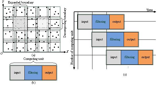

1. Introduction

Airborne light detection and ranging (LiDAR) data has been widely used in many fields, such as digital elevation modeling [1], 3D city modeling [2,3], geological and geomorphologic surveys [4], and environmental control [5,6]. Filtering is one of the core components in LiDAR data processing softwares [7]. By far, various types of filtering algorithms have been developed to classify the point clouds into ground and non-ground returns [8]. However, most of them are computationally intensive and time consuming because of their iterative frameworks [9]. Moreover, the size of the input data is often many times larger than what can be accommodated by computer memory. This can overwhelm the algorithms used to manage and analyze the data [10]. For large area mapping projects, 60% to 80% of the labor is allocated to classification and quality control [11]. Conventional sequential filters often need to load all the LiDAR points into the main memory before processing. As a result, the I/O becomes a bottleneck when the point clouds are processed because it is impossible to load the entire dataset into the memory at one time due to the limitations of computer hardware. Additionally, data input and output consume a large portion of the total processing time. Therefore, development of efficient filters is urgently needed.

Locality is a fundamental characteristic of point clouds, which means that a certain location is influenced by its surrounding environment and thus can be theoretically understood from the first law of geography (i.e., everything is related to everything else, but close things are more related than distant things [12]). Based on our experiences, locality-sensitive filters yield better results than the other algorithms because they involve more local contextual information about the neighborhood of a point than the other filtering strategies. This idea is the basis of the proposed approach in this paper. Indeed, common filters, such as the progressive TIN densification (PTD) filter [13–15], the progressive morphological filter [16,17], and the slope-based filters [18], often operate on local neighborhoods [19]. Thus, these filters involve locality-sensitive algorithms that judge each point based on its neighboring points. Therefore, a locality-oriented model can be used to represent this kind of filters. A streaming schedule algorithm is used to coordinate the I/O events of the point streams with the computing units. Its adaptability to different distribution patterns is examined, and how the computing performance of the streaming filter varies with the configuration of the computing units. The rest of the paper is organized into five additional sections. Section 2 reviews the relevant research on multi-core computing and streaming processing of the point clouds. The streaming framework, including the locality-preserved point clouds decomposition and the streaming schedule algorithms, is described in Section 3. Section 4 presents the streaming PTD (SPTD) under this framework. Section 5 shows several validation experiments with a detailed discussion of the experimental results. Some conclusions are drawn in Section 6.

2. Backgrounds and Related Works

Parallel computing is becoming mainstream based on multi-core processors. Currently, multi-core architectures become attractive devices given current technological possibilities and known physical limitations [20].

2.1. Multi-Core Processor and Thread Level Parallel Computing

A multi-core processor is an integrated circuit (IC) to which two or more processors are attached for enhanced performance, reduced power consumption, and more efficient simultaneous processing of multiple tasks. It adopts scalable shared-memory multiprocessor architectures [21]. Each processor can independently read and execute program instructions. Multithreading has become one of the most common foundations upon which developers build parallel software to leverage the power of multi-core processor. However, direct threading is difficult and somewhat error-prone [22]. Fortunately, some high-level threading libraries, such as OpenMP (Open Multi-Processing) [23] and TBB (Threading Building Block) [24], offer powerful new ways to achieve high performance in multi-core architectures. OpenMP is an Application Programming Interface (API) that supports multi-platform shared-memory multiprocessing programming in C, C++, and Fortran on most processor architectures and operating systems. It uses a portable, scalable model that gives programmers a simple and flexible interface for developing parallel applications for platforms ranging from the standard desktop computer to the supercomputer. TBB is a template library for C++ developed by Intel to parallelize programs. It is available in an open source version, as well as in a commercial version that provides further support. In special classes, parallel code is encapsulated and invoked from the program. As a result, development using these libraries is easier and more convenient because the low level complexities are hidden.

2.2. Streaming Processing of the Point Clouds

As stated by Jayasena [25], to simulate the large scale phenomena over long periods with increasing precision in fields such as biotechnology and climate modeling, there are great demands on high performance computing systems. Similarly, massive point clouds with increasing precision need to integrate the advantages of computing capacity for fast mapping and spatial analysis. Parallel computing can meet this need. However, conventional parallel computation uses batch processing on static data, such as the MapReduce model [26]. Although this paradigm is efficient, the large memory utilization is a non-trivial limitation, especially for processing massive point clouds on standalone machines.

As suggested by Stephens [27], stream processing system is composed of a collection of separate but communicating processes that receive stream data as input and produce stream data as output. In contrast with batch processing, stream computing views the data as a sequence of elements made available over time, allowing elements to be processed one by one rather than in large batches [28,29]. Stream computing may be a good fit for modern general-purpose processors for the following reasons [30]: (1) several modern micro-architectural features directly map to stream programming paradigm; (2) stream processing enables the arithmetic logic unit to execute at maximum efficiency in the operate stage; and (3) stream programming style greatly helps compilers with the traditionally very challenging task of scheduling the operation of hardware resources to maximize performance. Regarding the point clouds processing, more attention has been paid to stream computing processes, such as streaming Triangulated Irregular Network (TIN) generation [10,31], streaming Digital Elevation Model (DEM) generation [32], streaming interpolation [22], and stream-based building reconstruction [33]. In the field of point clouds processing, good spatial coherence can be utilized for the streaming process [10]. Similarly, most filters can be improved using streaming computing.

2.3. Related Parallel Filters

Parallel computing technologies have been introduced to speed up the filtering process. Han et al. [34] proposed a parallel processing method for interpolation of LiDAR point cloud using a PC cluster and a virtual grid, where the filtering is considered. The MapReduce programming model, introduced by Google, has also been evaluated by implementing a local gridding algorithm for the generation of DEM from point cloud data [35]. Hu et al. [36] proposed a simple scan-line-based algorithm using parallel computing. This algorithm works well in terms of both error rate and time performance for processing the points from non-mountainous areas. In addition, the support for Graphical Processing Units (GPUs) using Computed Unified Device Architecture (CUDA) and OpenCL was to be added into the point cloud library (PCL) [37].

PTD filter is one of the most commonly used and effective methods [15]. However, it is difficult to parallelize this algorithm due to the iterative combination of the triangulation and judging functions [36]. Different from Hu et al.’s opinion [36], parallelization of triangulation and judging by leveraging the multi-core architectures in a streaming way will be addressed in this paper. Moreover, the divide and conquer (D&C) method for triangulation is employed herein rather than the incremental insertion method.

3. The Multi-Core-Enabled Streaming Framework for Filtering Point Clouds

The multi-core-enabled streaming framework (Figure 1) is suitable for all the locality-based filters discussed in Section 1. In Figure 1a, the raw points are decomposed into overlapped blocks which are used as the input of the framework. In Figure 1b, each computing unit is used to encapsulate an inputting block and the filtering process, and scheduling of the computing units is shown in Figure 1c.

3.1. Locality-Preserved Spatial Decomposition

According to Yang et al. [38], increasing volume of data results in the kinds of extremes for a system to handle the data, and an ideal strategy is to divide the data set into small blocks with some duplication by extending the boundary of each block. In this way the decomposition enables the data blocks to be handled by computing resources in parallel. At the same time, the spatial principles can be used to facilitate fast access to large scale spatially continuous data.

Herein, the points are first decomposed into a series of blocks (see Figure 1a), and each block is surrounded by the decomposing boundaries. Then, to preserve the locality of the points around the boundary, each block is expanded by certain buffers which form the expanded boundaries (note: the expanded boundaries belonging to adjacent blocks are overlapped). Finally, the spatial extent is decomposed into some overlapped blocks, and each block is processed by a computing unit (see Section 3.2). In the following processing, points within the expanded boundaries are used for triangulation, and points within the decomposing boundaries are judged. In other words, the extent of triangulation is slightly larger than the extent of judging for the points of each block. In our experience, a value between 1% and 2% is enough for the overlapping between the blocks if a block is with a 1 km width and 1 km height.

3.2. Computing Unit

After decomposition, a filter can be used as the kernel algorithm for filtering the point clouds in each block. The filter plays the role of the computing unit, which can be a sequential or parallelized filter. Each filter takes the decomposing blocks as the input and returns the corresponding classified blocks as output.

Filtering accuracy has a priority for processing the point clouds. Generally, iteration-based filters have high accuracies. Some filters classify the points at a time, such as the slope-based filters [39,40], while some other filters [13–15,41–44] classify the points in multiple passes. The advantage of a single step algorithm is computational speed, which is traded for accuracy by iterating the solution, with the rationale that in each pass more information is gathered about the neighborhood of a point and thus a much more reliable classification can be obtained [19]. Herein, an iterative filter is selected as the kernel algorithm.

Moreover, efficiency is a key factor for filtering the point clouds. Thus, parallel computing is employed to improve the efficiency of the kernel filter (see Section 4 for details).

3.3. Streaming Schedule Strategy

To support the streaming filtering process, a block reader (R) and a result writer (W) are constructed. The reader R is able to continuously read points from the file and produce a series of overlapped blocks. These blocks are transferred to the subsequent computing units. Once a block has been processed by a computing unit, the result block is transferred to the writer, W. The filtering process performs in a fixed sequence, i.e., reader → computing unit → writer, and thus the streaming schedule strategy is termed as RCUW (reader, computing unit, and writer) (see Figure 2). Particularly, the reader R plays a role of a producer and pushes the produced blocks into a block queue. Additionally, each computing unit plays a dual role, both as a consumer processing the blocks in the block queue, and as a producer producing the result blocks and pushing them into the result queue. Comparably, the writer W plays a role of consumer for the computing units, and it is in charge of dumping the available data in the result queue into the output file. As a matter of fact, the framework contains two implicit threads: a reading thread and a writing thread, and these two threads are responsible for reading and writing respectively.

4. Multi-Core-Enabled PTD

The classic PTD filter is able to separate the points on the ground surface from the other points [14,15,19,45]. Due to its superior quality and adaptability, it has been used in TerraScan [13], a main component of the TerraSolid software family for processing LiDAR point clouds [46]. However, it is particularly computationally intensive, memory intensive, and time consuming, which poses a great challenge for processing massive point clouds [9]. Thus, the classic PTD filter needs to be improved in computation speed.

The classic PTD is an iterative process, and each iteration starts with building a new TIN representing the terrain model. In the iteration, the judging of each unclassified point is performed to determine the point belonging to the ground class or the object class. The iteration ends when no more ground points is detected. Thus, to improve the efficiency of PTD a direct way is to parallelize the triangulation and the judging functions, as well as to schedule the I/O events efficiently by means of the locality in the computation. By the above streaming framework, in Section 3, the SPTD is proposed, which leverages the power of multi-core processing to improve the practical performance of massive point clouds processing. In SPTD, parallel triangulation and parallel judging functions are packaged into a computing unit.

4.1. Parallelization of the Triangulation

Generally, streaming TIN and parallelization of the D&C triangulation algorithm are two common methods for parallelizing the triangulation. Herein, the latter is selected.

Streaming TIN generation algorithms provide a potential method for triangulating the point clouds. Wu et al. [31] developed an algorithm called ParaStream for Delaunay triangulation via integrating the streaming computing with the D&C triangulation method. ParaStream can attain a speedup of about 6.8 times with lower memory footprint [31]. Streaming TIN, developed by Isenburg et al., employs the incremental insertion method for triangulation, and very low memory footprint is its advantage when processing the voluminous point clouds [10]. From the perspective of efficiency, Parastream outperforms the other. However, the process of streaming TIN generation conflicts with the iterative nature of the PTD. The PTD filter needs to progressively add terrain points into the TIN in completely random places; however, this cannot be allowed in Parastream. In addition, the multi-grid solver for reading the irregular meshes [47] can produce the locality from the existed meshes; however, the reading process is insufficient for the need of iterative densification and re-triangulation. Consequently, streaming TIN generation is not adopted in our method.

As stated by Chrisochoides [48], parallel algorithms for Delaunay triangulation can be classified into three categories: (i) algorithms that first mesh the interfaces of sub-problems and then mesh the individual sub-problems in parallel, (ii) algorithms that first solve the meshing problem for each of the sub-problems in parallel and then mesh the interfaces, so that the global mesh is conforming, and (iii) algorithms that simultaneously mesh and improve the interfaces as they mesh the individual sub-problems. Essentially, all these algorithms adopt the D&C strategy, which provides a natural way to parallelize the triangulation. Su and Drysdale [49] found that the D&C algorithm is the fastest among the existing triangulation algorithms, with the sweep line algorithm second. The incremental algorithm performs poorly because it spends most of its time locating points. In this paper, the parallel D&C triangulation is adopted.

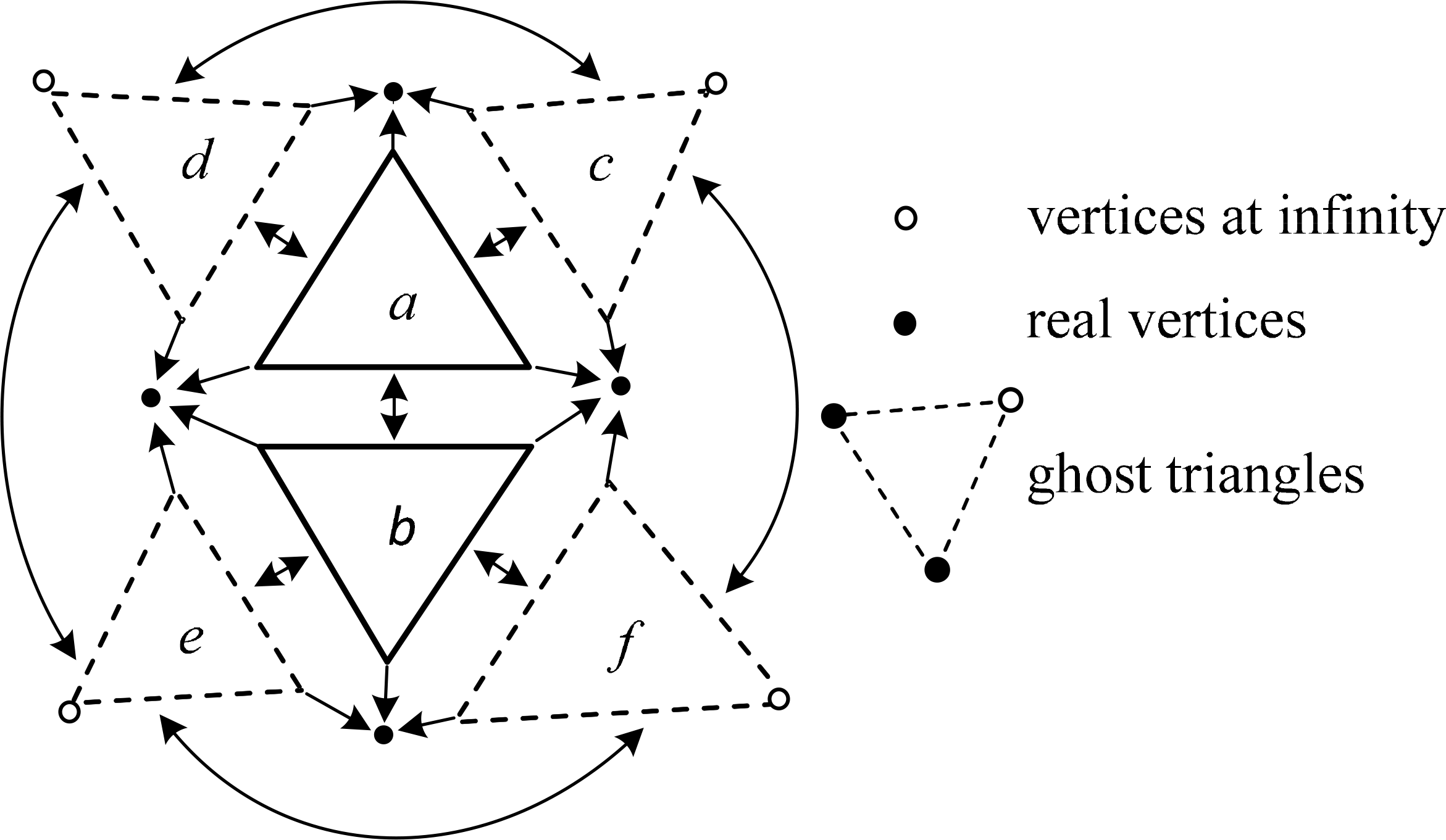
As an open source package for two-dimensional Delaunay triangulation, “Triangle” simultaneously implements the D&C algorithm, the sweep line algorithm, and the incremental algorithm [50]. The D&C algorithm is, herein, selected to parallelize the triangulation. The data structure is illustrated as follows (see Figure 3). Each triangle contains three pointers to the neighboring triangles and three pointers to the vertices. In Figure 3, the white vertices represent the “vertices at infinity”. Only the black vertices have coordinates. A ghost triangle is made up of a white vertex and two black vertices, and it is used for the following merging process in triangulation.

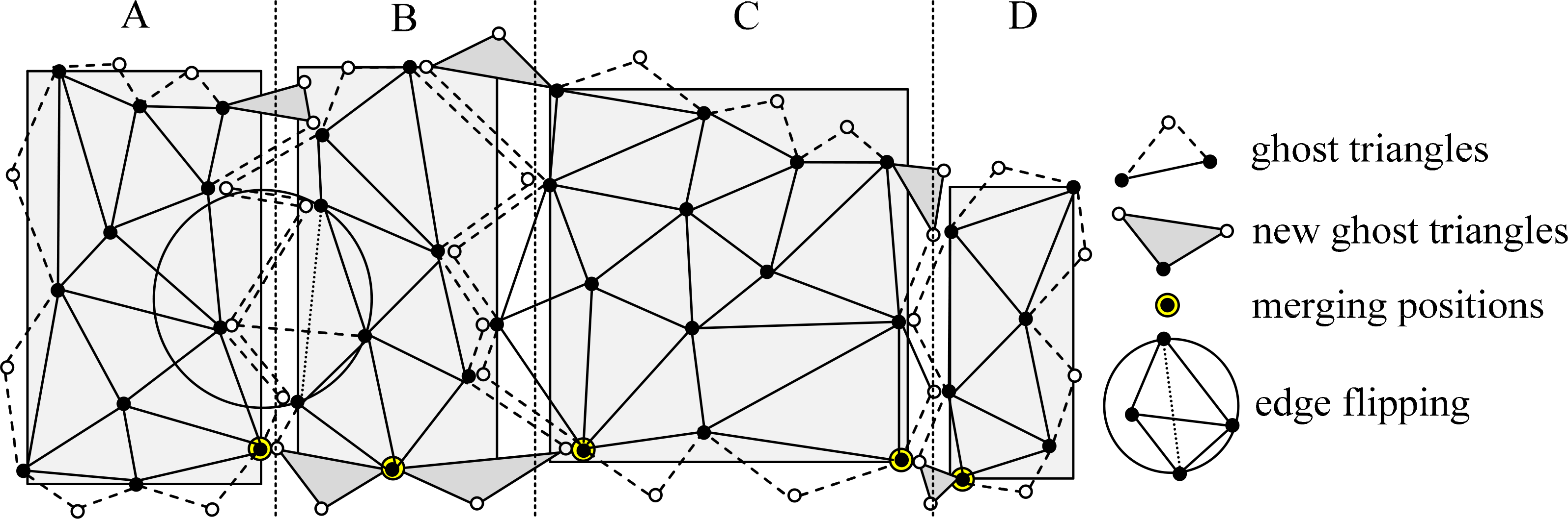
Before D&C-based triangulation, an initialized step is used to sort the input points in ascending order by either their x-coordinates or their y-coordinates. After sorting, the duplicated points in each plane coordinate are eliminated except for the lowest point, because the other duplicated points may cause confusion in the triangulation mesh generated by “Triangle”. The lowest point is the most likely point to be used as the ground point, and it is therefore preserved. Subsequently, the points are recursively halved until each subset has only two or three points. At this moment, each subset can be easily triangulated. The sub-meshes will also be merged to form larger meshes recursively. To exploit the parallelism in D&C, the entire point set is partitioned into multiple subsets, each with the same number of points, and then each of them is triangulated in parallel. Finally, a merging procedure is performed to merge the neighboring sub-meshes to form the entire mesh. The merging procedure includes three steps: (i) traversing the ghost triangles counter-clockwise and locating the two bottom points of the two neighboring sub-meshes, (ii) fitting together the ghost triangles like the teeth of two gears from the two bottom points, and (iii) refining the non-Delaunay triangles by flipping the edges. The computing time of the sequential triangulation algorithm in the open source package “Triangle” can be modeled as follows [50]:

$$T_S^{\mathit{Triangulation}}=O(n\text{log}n)$$

(1)

where n represents the number of vertices.

As shown in Figure 4, the points are first partitioned into four subsets (A, B, C, and D). Then, the four subsets are triangulated in parallel by sequential D&C. After the triangulation of each subset, the final merging procedure is used to merge the neighboring sub-meshes along with the ghost triangles. Finally, the ghost triangles are removed, and the final triangulation mesh is formed.

To alleviate the competition from frequent memory allocating, the memory structure of the original “Triangle” is rewritten and the triangle elements are allowed to be independently allocated and modified in the memory space. During the parallel triangulation, each of the threads is given an independent block of memory to allocate for the newly created triangles. Thus, these multiple threads can concurrently triangulate the points and there is no competition in memory allocation. At last, the merging procedure generates some triangles in a sequential way. Therefore, the triangulations of the different subsets are independent on each other, allowing better efficiency to be achieved.

Table 1. Pseudo-code for parallel triangulation.

1.	Sort the input points in ascending order by either their x-coordinates or their y-coordinates;
2.	Divide the points into N subsets with equal size;
3.	For n = 1 to N do in Parallel. {Triangulate each subset and form N triangulations;}
4.	For n = 1 to N − 1. Merge the adjacent triangulations in a sequential way;
5.	Output the final triangulation

shows the pseudo-code.

The computing time of the proposed parallel triangulation algorithms could be therefore modeled by:

$$T_P^{\mathit{Triangulation}}=O(\frac{n}{p}\text{log}n)$$

(2)

where p is the number of processors.

To realize the parallelization of the multiple judging functions in each point block, the triangulation in each block should be independent, which guarantees the streaming framework to fit for filtering the point clouds. In other words, the independent parallelization of the triangulation is special for the streaming filter, SPTD.

4.2. Parallelization of the Judging Functions

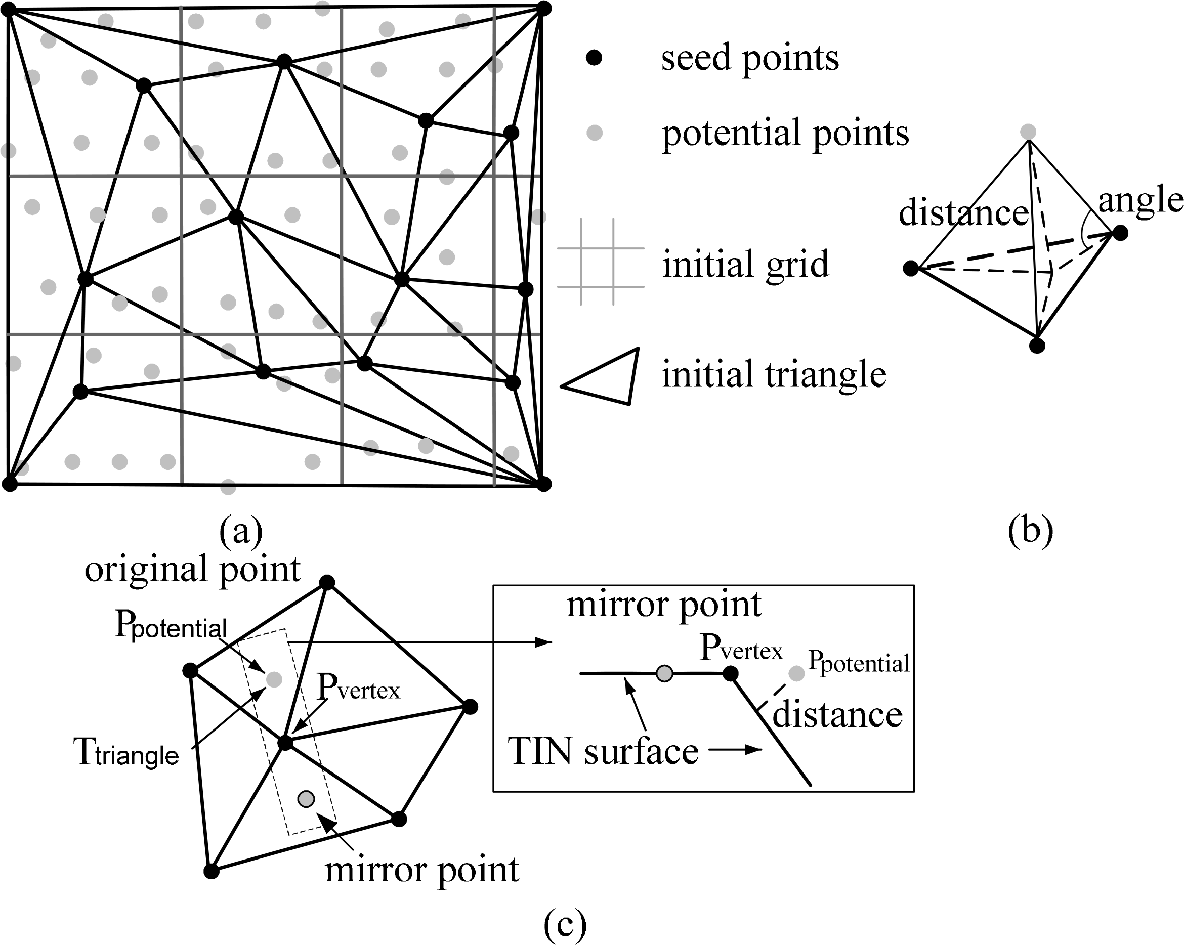
The classic PTD is composed of four core steps [13–15]: (i) calculating the initial parameters using the points set, (ii) selecting the seed points set, (iii) iterative densification of the TIN using some judging functions, and (iv) iteration until all the points are classified as ground or object. The second step is to get initial ground points from each grid (see Figure 5a). The third step is to calculate the angles and distances from the points included in the TIN (see Figure 5b), and the points below the threshold value of the TIN are added. For a discontinuous surface, additional calculations are introduced to handle the problems of edge cutting-off. As shown in Figure 5c, the original point, P, is mirrored to the closest vertex for further calculation. The calculation of angles and distances is the key step for speeding up the processing. According to the analysis of the judging process, the computing time of the sequential judging functions could be modeled by:

$$T_S^{\mathit{Judging}}=O(n)$$

(3)

where n is the number of the points. The parallelization of these calculations is described herein.

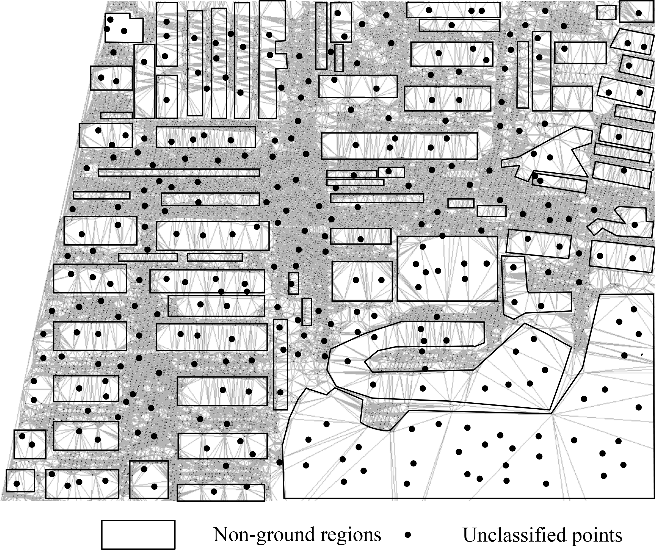
After the first time of densification, the triangulation mesh built from the ground points often takes on a non-uniform morphology. The distribution of the ground points is non-uniform due to the existence of objects in the real world scenes that produce either locally dense meshes or locally sparse meshes (see Figure 6). As shown in Figure 6, ground points are missing in the building regions. After triangulation, a huge number of small triangles are clustered in these pure terrain regions. However, some large triangles exist inside or across the buildings. Correspondingly, the computational burdens vary greatly for the triangles in different local regions of the real world scenes; so assigning triangles into different cores is a key for balancing the sub-tasks. To assign these aggregated or decentralized triangles into the parallel computing threads in a well balanced way, modulo-N arithmetic represents a direct and easy way to assign triangulation meshes into N subsets according to the triangle identifiers (see the pseudo code in

Table 2. Pseudo-code for the parallel judging function.

1.	Initialize the input point set S, the output point set S’, and triangulation T;
2.	Divide the spatial extent of S into a uniform grid, and select the seeds set U from the grids:S’ = U, S = S − U;
3.	Build the initial triangulation T with S’;
4.	Iteratively judging the points in S: While (S is not empty) {Divide T into N subset: $T={\sum }_{n=1}^N{T}_n(n)$; For n = 1 to N do in Parallel {Take out a triangle t ∈ Tn; Find the points G that are located in t; Calculate angles (α, β, γ) and distance (d) for the points in G and get the ground points G’; Add G’ into S’: S’ = S’ + G’, S = S – G’;} Clear T and re-triangulate the S’ for T;}
5.	Clear S, T, and output S’;

). In this way, each local region represented by clustering triangles with high or low computational burden is discretely divided into different subsets to form a sub-task.

A formal description of the parallel version of the PTD is illustrated in Table 2. The input point set, S, is composed of the initial unclassified ground and non-ground points. After filtering, the classified points are stored in the point set S’. T is the triangle set which is updated in each of the iterative judging pass. U is the seed point set.

In the initialization step of the proposed filtering method, each point is assigned a grid, and the size of each grid is equal to a constant threshold (the maximum size of the buildings). The above grid index is constructed to fasten the process for finding the points in some triangles. Particularly, the number of points in each grid is relatively invariant. For example, if the grid size is six meters and the average point density is 1 point/m², each grid contains about 36 points. Once the TIN is constructed, the relevant grids could be determined for each triangle if the grids are intersected with or contain the triangle, as shown in Figure 5a. Then, only the points that belonging to these relevant grids should be analyzed for the locating process. In this sense, the locating of a point in some triangle is a constant-time operation, and the needed time is determined by both of the maximum size of the buildings and the average point density. In addition, the number of the triangles is positively proportional to the number of the points, and thus judging a point within a triangle is also a constant-time operation. Obviously, the computing time of the parallel judging functions can be modeled as follows:

$$T_P^{\mathit{Judging}}=O(\frac{n}{p})$$

(4)

4.3. Computational Complexity

The SPTD is partially composed of the parallel triangulation algorithms and the parallel judging algorithms. On the whole, the computational complexity can be modeled by Equation (5) based on Equation (2) and Equation (4):

$$T_P=\left(T_P^{\mathit{Triangulation}}+T_P^{\mathit{Judging}}\right)=O\left(\frac{n\text{log}n}{p}\right)+O\left(\frac{n}{p}\right)=O\left(\frac{n\text{log}n}{p}\right)$$

(5)

5. Experiments and Analysis

5.1. Experiment Environment and Datasets

The experiments are conducted on a workstation running Microsoft Windows 7 (× 64) with two Six-Core Intel Xeon E5645 (2.40 GHz in each core), 16 GB DDR3-1333 ECCSDRAM and a 2 TB hard disk (7200 rpm, 64 MB cache). OpenMP is used for thread-level parallelism. In addition, Hyper-Threading Technology makes a single physical processor appear as two logical processors; the physical execution resources are shared and the architecture state is duplicated for the two logical processors [51]. Therefore, the maximum number of threads for the two processors is 24. The program is compiled with the Intel C++ compiler.

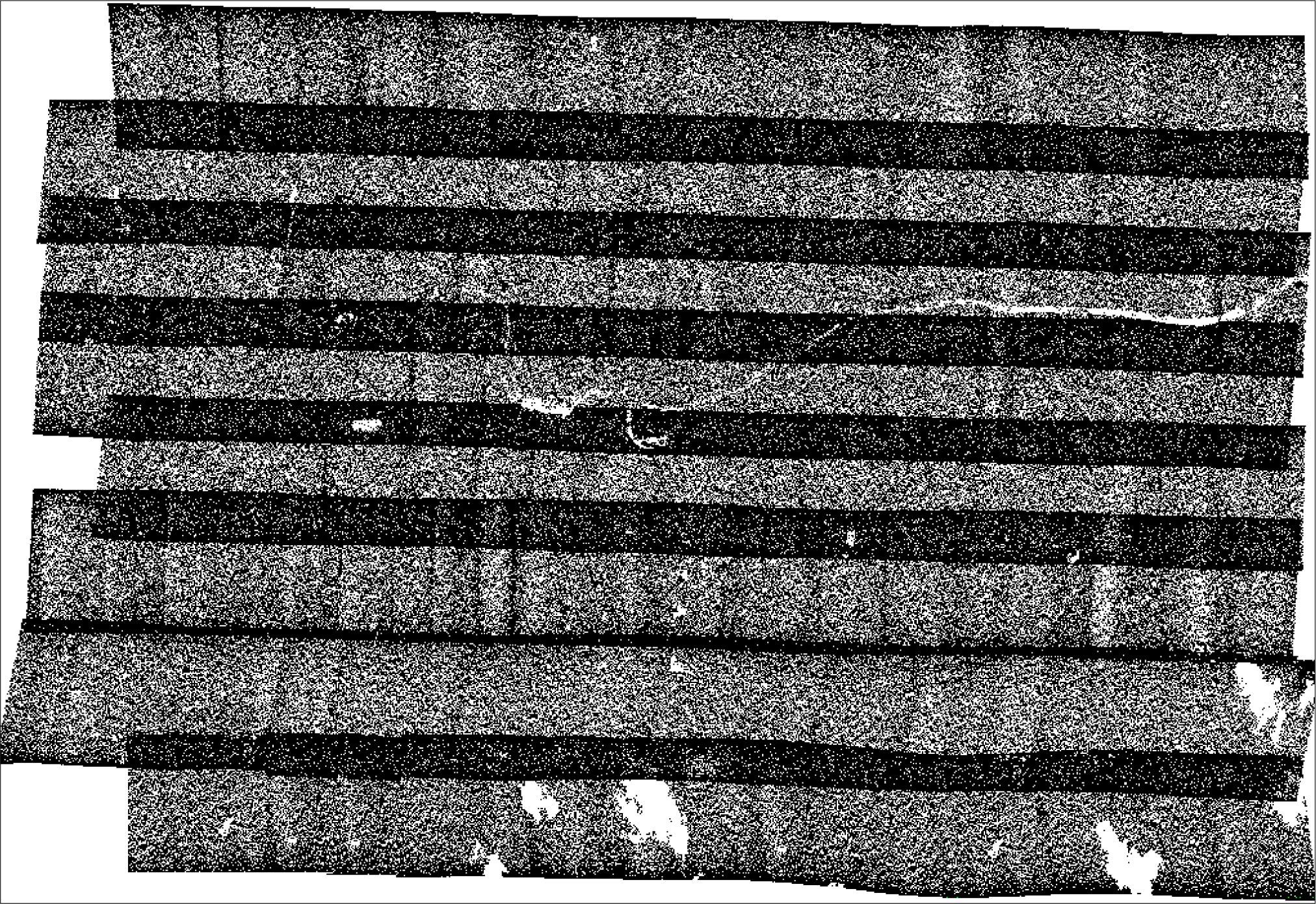
The datasets include three small datasets and a large dataset. Each of the small datasets contains about 7.9 million points; the large dataset contains about 249 million points. The first small dataset covers a uniformly distributed region in Dalian City (see Figure 7a). Moreover, to verify the idea in Section 4.2 that the assignment of modulo-N arithmetic in the computing units can contribute to a better adaptability, the other two small datasets with normal distribution (see Figure 7b) and cluster distribution (see Figure 7c) are generated by sampling a real-world point cloud data set, respectively. The larger dataset is covered within Anyang City (see Figure 8), Henan Province, China, and it occupies 7.20 GB of external space. As shown in Figure 8, the point density is not uniform for the overlapping of the eight LiDAR strips.

Moreover, an extra preprocessing is performed in two passes to decompose the spatial extent into overlapped blocks for Anyang dataset. In the first pass, the points are traversed, and both of the number of the points and the spatial extent are computed for the dataset. In the second pass, the spatial extent is decomposed, and each point is allocated into a block or multiple blocks.

5.2. Experimental Results

Using modern accelerator technologies to speed up remote sensing data processing has become a main trend [52]. To verify the performance of the SPTD, two groups of experiments have been carried out. Moreover, speedup is used to measure the efficiency, and it can be defined by the following equation [53]:

$$S_p=\frac{T_1}{T_p}$$

(6)

where p is the number of processors; T₁ is the execution time of the sequential algorithm; T_p is the execution time of the parallel algorithm with p processors. The first group of experiments is used to examine the adaptability of the computing unit to the distribution patterns of the three datasets, and the results refer to

Table 3. The time and speedup of a computing unit in different number of threads to the datasets with different distribution patterns.

Number of Threads	Uniform Distribution		Normal Distribution		Cluster Distribution
	Time (s)	Speedup	Time (s)	Speedup	Time (s)	Speedup
1	37.2	1.0	37.6	1.0	38.0	1.0
2	20.1	1.9	20.1	1.9	19.8	1.9
4	14.2	2.6	14.3	2.6	16.7	2.3
6	13.6	2.7	13.2	2.8	13.9	2.7
8	14.1	2.6	14.2	2.6	14.6	2.6
10	13.9	2.7	14.1	2.7	14.6	2.6
12	13.6	2.7	13.8	2.7	14.1	2.7

. Table 3 suggests that, compared with the uniform distribution, there are no obvious fluctuations in the speedup when the point cloud datasets with normal distribution and cluster distribution are filtered, respectively. For example when the number of threads is 6, the speedup of the three datasets with the uniform distribution, normal distribution, and cluster distribution are 2.7, 2.6, and 2.8, respectively. The above three values are equivalent.

Table 4. The time usage of the triangulation and the judging in different number of threads to the dataset with uniform distribution pattern.

Number of Threads	Time (s)	Triangulation		Judging
		Time (s)	Percentage (%)	Time (s)	Percentage (%)
1	37.2	7.7	20.7	29.5	79.3
2	20.1	4.2	20.9	15.9	79.1
4	14.2	2.5	17.6	11.7	82.4
6	13.6	1.7	12.5	11.9	87.5
8	14.1	1.5	10.6	12.6	89.4
10	13.9	1.3	9.4	12.6	90.6
12	13.6	1.1	8.1	12.5	91.9
Average			14.3		85.7

shows the time used in the triangulation and the judging to the dataset with uniform distribution pattern. Table 4 suggests that, compared with the judging algorithms, the time used in the triangulation takes up only a small portion of the total time.

The second group of the experiments is used to examine the efficiency of the SPTD in processing massive point clouds within a 12-core computing environment. Each core is permitted to allocate double threads for the Hyper-Threading Technology. Thus, there is a maximum of 24 threads. These 24 threads are evenly assigned to multiple computing units. In the experiments, the number of the computing units is assigned to 1, 2, 4, 6, 12, and 24, respectively. Correspondingly, the statistics of the computing time, the peak memory usage, and the speedup for different number of threads per computing unit in each assignment refer to

Table 5. The statistics of the computing time, the peak memory usage and speedup when the number of computing units is equal to 1.

Number of Threads per Computing Unit	Time (s)	Peak Memory Usage	Speedup
1	-	memory allocation failure	-
2	-	memory allocation failure	-
4	-	memory allocation failure	-
6	265.9	9465	2.5
12	259.6	10,668	2.6
24	261.2	11,052	2.6

Table 6. The statistics of the computing time, the peak memory usage and speedup when the number of computing units is equal to 2.

Number of Threads per Computing Unit	Time (s)	Peak Memory Usage	Speedup
1	-	memory allocation failure	-
2	199.3	10,223	3.4
4	171.1	6807	3.9
6	168.9	9874	4.0
12	168.0	5065	4.0

Table 7. The statistics of the computing time, the peak memory usage and speedup when the number of computing units is equal to 4.

Number of Threads per Computing Unit	Time (s)	Peak Memory Usage	Speedup
1	184.0	6905	3.7
2	137.7	3095	4.9
4	113.5	2286	5.9
6	124.2	868	5.4

Table 8. The statistics of the computing time, the peak memory usage and speedup when the number of computing units is equal to 6.

Number of Threads per Computing Unit	Time (s)	Peak Memory Usage	Speedup
1	132.1	3513	5.1
2	103.7	1313	6.5
4	107.4	874	6.3

Table 9. The statistics of the computing time, the peak memory usage and speedup when the number of computing units is equal to 12.

Number of Threads per Computing Unit	Time (s)	Peak Memory Usage	Speedup
1	104.5	1519	6.5
2	96.7	1057	7.0

and

Table 10. The statistics of the computing time, the peak memory usage and speedup when the number of computing units is equal to 24.

Number of Threads per Computing unit	Time (s)	Peak Memory Usage	Speedup
1	101.1	1622	6.7

, respectively. Under the condition that the number of computing units is fixed, different numbers of computing threads are utilized to parallelize each computing unit. For example, Table 5 lists the values of the computing time, the peak memory usage, and the speedup when the number of threads per computing unit is equal to 1, 2, 4, 6, 12 respectively under the condition that the number of computing units is equal to 2. Thus, the efficiency of the SPTD can be reflected by the speedup in Tables 5 and 10. Moreover, the dot product of the number of computing units and the number of threads per computing unit should be less than or equal to 24 in Tables 5 and 10. For example, when the number of the computing units is equal to 4 in Table 6, the maximum number of threads per computing unit is 6.

Additionally, in order to calculate the speedup, a comparable filtering experiment in sequential mode is performed, which takes 674.6 s for the 249 million points. Moreover, the peak memory usage is about 168 MB.

As mentioned above, Tables 5 and 10 show the statistics of the running time, peak memory usage, and the speedup for different number of threads per computing unit when the number of the computing units is assigned to 1, 2, 4, 6, 12, and 24, respectively. For example in Table 9, the maximum speedup is 7.0 when the number of computing units is equal to 12, and the corresponding running time and peak memory usage is 96.7 s and 1057 MB, respectively. When the maximum speedup is obtained under the condition that the number of the computing units is assigned to 1, 2, 4, 6, 12, and 24, the corresponding running time and peak memory usage in Figure 9 suggests that both of the lower memory usage and the lower running time can be simultaneously obtained when the number of computing units is equal to 6, 12, and 24.

5.3. Discussion

Two groups of experiments have been given here. The first group of experiments evaluates the adaptability of the proposed computing unit to the point clouds with different distribution patterns. With the modulo-N arithmetic, the computing unit is more adaptable to different distribution patterns, and there are no significant differences in the efficiency of the computing units for the point clouds with uniform, normal and cluster distributions. This can attribute to modulo-N arithmetic which enables better loading balance among the subsets of the triangles.

The second group of experiments evaluates the efficiency of the SPTD in processing massive point clouds. According to Figure 9, an ideal performance is obtained when the I/O speed is matching with the filtering efficiency, i.e., the computing units can provide a consuming capacity compatible with the producing speed. If the point blocks cannot be consumed in time, memory usage increases sharply. In addition, more computing units should be allocated if the reader can produce the point blocks more quickly. Specifically, the second group of experiments can be understood from the relation between the number of the computing units and the corresponding time spent (as shown in Figure 9). In other words, when the speed of reading points by the reader, R, and the speed of judging the points by the computing units are compatible, the number of points to be processed is directly proportional to the computing time. Therefore, there is no need individually testing the program from the job size.

Furthermore, the two groups of experiments demonstrate that the judging algorithms cost more time than the triangulation in the SPTD. As stated in Section 4, the upper bound of the computational complexity in theory is determined by the parallel triangulation algorithms. However, the testing empirical results from Table 4 indicate that the judging algorithms cost more time than the parallel triangulation algorithms. The reasonable explanation is that the time used in judging a point is many times longer than the average time used in triangulation for each point.

6. Conclusions

A streaming framework for filtering the point clouds is proposed in this paper, which includes a reader, R, a writer, W, and multiple computing units. First, the point clouds is decomposed into slightly overlapped blocks, and then the reader R continuously loads the blocks and transfer them to the computing units. After processing, the output results are written back to the disk by the writer W. In this framework, locality-based progressive TIN densification is selected as the computing unit and parallelized using the multi-core architectures, which forms the streaming progressive TIN densification filter. Specifically, the computing unit is built through iteratively performing both of the triangulation and the judging. Two groups of experiments suggest an increase in speed of 7.0 times (including I/O time). Impressively, the time for processing 249 million points is reduced from 11.2 min to 1.6 min.

The main contributions of this study include two aspects: (i) the proposal of a general streaming framework for parallelizing locality-based filters; and (ii) the implementation of streaming progressive TIN densification that greatly alleviates the I/O bottleneck and improves the performance for processing massive point clouds. The future work will focus on the improvement of the proposed filter. For example, the markov random field model [54] might be introduced to analyze the spatial topology, and multi-source data fusion [55] is employed to increase the accuracy.

References

- Agarwal, P.; Arge, L.; Danner, A. From point cloud to grid dem: A scalable approach. In Progress in Spatial Data Handling; Riedl, A., Kainz, W., Elmes, G., Eds.; Springer: Berlin/Heidelberg, Germany, 2006; pp. 771–788. [Google Scholar]
- Wang, R. 3D building modeling using images and LiDAR: A review. Int. J. Image Data Fusion 2013, 4, 273–292. [Google Scholar]
- Hammoudi, K.; Dornaika, F.; Soheilian, B.; Paparoditis, N. Extracting wire-frame models of street facades from 3D point clouds and the corresponding cadastral map. International Archives of Photogrammetry, Remote Sensing and Spatial Information Sciences, Saint-Mandé, Paris, France, 1–3 September 2010; 38, pp. 91–96.
- Baldo, M.; Bicocchi, C.; Chiocchini, U.; Giordan, D.; Lollino, G. LIDAR monitoring of mass wasting processes: The Radicofani Landslide, Province of Siena, Central Italy. Geomorphology 2009, 105, 193–201. [Google Scholar]
- Charlton, M.; Large, A.; Fuller, I. Application of airborne LiDAR in river environments: The River Coquet, Northumberland, UK. Earth Surf. Process. Landf 2003, 28, 299–306. [Google Scholar]
- Young, A.P.; Ashford, S.A. Application of airborne LIDAR for seacliff volumetric change and beach-sediment budget contributions. J. Coast. Res 2006, 22, 307–318. [Google Scholar]
- Shen, J.; Liu, J.; Lin, X.; Zhao, R. Object-based classification of airborne light detection and ranging point clouds in human settlements. Sens. Lett 2012, 10, 221–229. [Google Scholar]
- Zhang, J.; Lin, X.; Ning, X. SVM-based classification of segmented Airborne LiDAR point clouds in urban areas. Remote Sens 2013, 5, 3749–3775. [Google Scholar]
- Chen, Q. Airborne LiDAR data processing and information extraction. Photogramm. Eng. Remote Sens 2007, 73, 109–112. [Google Scholar]
- Isenburg, M.; Liu, Y.; Shewchuk, J.; Snoeyink, J. Streaming computation of delaunay triangulations. Proceedings of the ACM SIGGRAPH 2006 Papers, Boston, MA, USA, 30 July–03 August 2006; pp. 1049–1056.
- Flood, M. LiDAR activities and research priorities in the commercial sector. Int. Arch. Photogramm. Remote Sens 2001, 34, 3–8. [Google Scholar]
- Tobler, W.R. A computer movie simulating urban growth in the Detroit region. Econ. Geogr 1970, 46, 234–240. [Google Scholar]
- Axelsson, P. DEM generation from laser scanner data using adaptive TIN models. Int. Arch. Photogramm. Remote Sens 2000, 33, 111–118. [Google Scholar]
- Zhang, J.; Lin, X. Filtering airborne LiDAR data by embedding smoothness-constrained segmentation in progressive tin densification. ISPRS J. Photogramm. Remote Sens 2013, 81, 44–59. [Google Scholar]
- Lin, X.; Zhang, J. Segmentation-based filtering of airborne LiDAR point clouds by progressive densification of terrain segments. Remote Sens 2014, 6, 1294–1326. [Google Scholar]
- Zhang, K.; Chen, S.-C.; Whitman, D.; Shyu, M.-L.; Yan, J.; Zhang, C. A progressive morphological filter for removing nonground measurements from airborne LiDAR data. IEEE Trans. Geosci. Remote Sens 2003, 41, 872–882. [Google Scholar]
- Pirotti, F.; Guarnieri, A.; Vettore, A. Ground filtering and vegetation mapping using multi-return terrestrial laser scanning. ISPRS J. Photogramm. Remote Sens 2013, 76, 56–63. [Google Scholar]
- Vosselman, G. Slope based filtering of laser altimetry data. Int. Arch. Photogramm. Remote Sens 2000, 33, 935–942. [Google Scholar]
- Sithole, G.; Vosselman, G. Experimental comparison of filter algorithms for bare-earth extraction from airborne laser scanning point clouds. ISPRS J. Photogramm. Remote Sens 2004, 59, 85–101. [Google Scholar]
- Valiant, L. A bridging model for multi-core computing. In Algorithms—Esa 2008; Halperin, D., Mehlhorn, K., Eds.; Springer: Berlin/Heidelberg, Germany, 2008; Volume 5193, pp. 13–28. [Google Scholar]
- Lenoski, D.E.; Weber, W.-D. Scalable Shared-Memory Multiprocessing; Morgan Kaufmann Publishers: San Francisco, CA, USA, 1995; Volume 1006. [Google Scholar]
- Guan, X.; Wu, H. Leveraging the power of multi-core platforms for large-scale geospatial data processing: Exemplified by generating DEM from massive LiDAR point clouds. Comput. Geosci 2010, 36, 1276–1282. [Google Scholar]
- Dagum, L.; Menon, R. Openmp: An industry standard api for shared-memory programming. IEEE Comput. Sci. Eng 1998, 5, 46–55. [Google Scholar]
- Reinders, J. Intel Threading Building Blocks: Outfitting C++ for Multi-Core Processor Parallelism; O’Reilly Media, Inc.: Sebastopol, CA, USA, 2007. [Google Scholar]
- Jayasena, N.S. Memory Hierarchy Design for Stream Computing; Stanford University: Stanford, CA, USA, 2005. [Google Scholar]
- Dean, J.; Ghemawat, S. Mapreduce: Simplified data processing on large clusters. Commun. ACM 2008, 51, 107–113. [Google Scholar]
- Stephens, R. A survey of stream processing. Acta Inform 1997, 34, 491–541. [Google Scholar]
- Feigenbaum, J.; Kannan, S.; Strauss, M.J.; Viswanathan, M. An approximate L1-difference algorithm for massive data streams. SIAM J. Comput 2002, 32, 131–151. [Google Scholar]
- Neumeyer, L.; Robbins, B.; Nair, A.; Kesari, A. S4: Distributed stream computing platform. Proceedings of the IEEE International Conference on Data Mining Workshops (ICDMW), Sydney, Australia, 13 December 2010; pp. 170–177.
- Gummaraju, J.; Rosenblum, M. Stream processing in general-purpose processors. Proceedings of the 11th International Conference on Architectural Support for Programming Languages and Operating Systems (ASPLOS 04’), Boston, MA, USA, 9–13 October 2004.
- Wu, H.; Guan, X.; Gong, J. Parastream: A parallel streaming delaunay triangulation algorithm for LiDAR points on multicore architectures. Comput. Geosci 2011, 37, 1355–1363. [Google Scholar]
- Isenburg, M.; Liu, Y.; Shewchuk, J.; Snoeyink, J.; Thirion, T. Generating raster dem from mass points via tin streaming. In Geographic Information Science; Raubal, M., Miller, H., Frank, A., Goodchild, M., Eds.; Springer: Berlin/Heidelberg, Germany, 2006; Volume 4197, pp. 186–198. [Google Scholar]
- Zhou, Q.-Y.; Neumann, U. A streaming framework for seamless building reconstruction from large-scale aerial LiDAR data. Proceedings of the IEEE Conference on Computer Vision and Pattern Recognition, 2009, (CVPR 2009). Miami, FL, USA, 20–25 June 2009; pp. 2759–2766.
- Han, S.H.; Heo, J.; Sohn, H.G.; Yu, K. Parallel processing method for airborne laser scanning data using a PC cluster and a virtual grid. Sensors 2009, 9, 2555–2573. [Google Scholar]
- Krishnan, S.; Baru, C.; Crosby, C. Evaluation of mapreduce for gridding LiDAR data. Proceedings of the Conference on 2010 IEEE Second International Cloud Computing Technology and Science (CloudCom), Indianapolis, IN, USA, 30 December 2010; pp. 33–40.
- Hu, X.; Li, X.; Zhang, Y. Fast filtering of LiDAR point cloud in urban areas based on scan line segmentation and GPU acceleration. IEEE Geosci. Remote Sens 2013, 10, 308–312. [Google Scholar]
- Rusu, R.B.; Cousins, S. 3D is here: Point Cloud Library (PCL). Proceedings of the IEEE International Conference on Robotics and Automation, Shanghai, China, 41–. 18 May 2011; pp. 1–4.
- Yang, C.; Wu, H.; Huang, Q.; Li, Z.; Li, J. Using spatial principles to optimize distributed computing for enabling the physical science discoveries. Proc. Natl. Acad. Sci. USA 2011, 108, 5498–5503. [Google Scholar]
- Sithole, G. Filtering of laser altimetry data using a slope adaptive filter. ISPRS J. Photogramm. Remote Sens 2001, 34, 203–210. [Google Scholar]
- Roggero, M. Airborne laser scanning-clustering in raw data. Int. Arch. Photogramm. Remote Sens 2001, 34, 227–232. [Google Scholar]
- Sohn, G.; Dowman, I. Terrain surface reconstruction by the use of tetrahedron model with the MDL criterion. Int. Arch. Photogramm. Remote Sens 2002, 34, 336–344. [Google Scholar]
- Brovelli, M.; Cannata, M.; Longoni, U. Managing and processing LIDAR data within GRASS. Proceedings of the GRASS Users Conference, Trento, Italy, 11–13 September 2002.
- Pfeifer, N.; Köstli, A.; Kraus, K. Interpolation and filtering of laser scanner data-implementation and first results. Int. Arch. Photogramm. Remote Sens 1998, 32, 153–159. [Google Scholar]
- Elmqvist, M. Ground surface estimation from airborne laser scanner data using active shape models. Int. Arch. Photogramm. Remote Sens 2002, 34, 114–118. [Google Scholar]
- Zhu, X.; Toutin, T. Land cover classification using airborne LiDAR products in beauport, Québec, Canada. Int. J. Image Data Fusion 2013, 4, 252–271. [Google Scholar]
- Soininen, A. Terrascan User’s Guide; The National Mapping Agency of Great Britain: Southampton, UK, 2012. [Google Scholar]
- Shi, X.; Bao, H.; Zhou, K. Out-of-core multigrid solver for streaming meshes. Proceedings of the ACM SIGGRAPH Asia 2009 papers, Yokohama, Japan, 16–19 December 2009; ACM: New York, NY, USA; pp. 1–7.
- Chrisochoides, N. Parallel mesh generation. In Numerical Solution of Partial Differential Equations on Parallel Computers; Bruaset, A., Tveito, A., Eds.; Springer: Berlin/Heidelberg, Gremany, 2006; Volume 51, pp. 237–264. [Google Scholar]
- Su, P.; Scot Drysdale, R.L. A comparison of sequential delaunay triangulation algorithms. Comput. Geom 1997, 7, 361–385. [Google Scholar]
- Shewchuk, J.R. Triangle: Engineering a 2D quality mesh generator and Delaunay triangulator. In Applied Computational Geometry Towards Geometric Engineering; Lin, M.C., Manocha, D., Eds.; Springer-Verlag: Berlin, Germany, 1996; pp. 203–222. [Google Scholar]
- Marr, D.T.; Binns, F.; Hill, D.L.; Hinton, G.; Koufaty, D.A.; Miller, J.A.; Upton, M. Hyper-threading technology architecture and microarchitecture. Int. Technol. J 2002, 6, 4–15. [Google Scholar]
- Shi, X.; Kindratenko, V.; Yang, C. Modern accelerator technologies for geographic information science. In Modern Accelerator Technologies for Geographic Information Science; Shi, X., Kindratenko, V., Yang, C., Eds.; Springer: New York, NY, USA, 2013; pp. 3–6. [Google Scholar]
- Rauber, T.; Rünger, G. Performance analysis of parallel programs. In Parallel Programming; Springer: Berlin/Heidelberg, Germany, 2013; pp. 169–226. [Google Scholar]
- Seetharaman, K.; Palanivel, N. Texture characterization, representation, description, and classification based on full range Gaussian Markov random field model with Bayesian approach. Int. J. Image Data Fusion 2013, 4, 342–362. [Google Scholar]
- Akiwowo, A.; Eftekhari, M. Feature-based detection using Bayesian data fusion. Int. J. Image Data Fusion 2013, 4, 308–323. [Google Scholar]