Remote Geophysical Observatory in Antarctica with HF Data Transmission: A Review

 , ,
, ,  ,
,
Abstract
: The geophysical observatory in the Antarctic Spanish Station, Juan Carlos I (ASJI), on Livingston Island, has been monitoring the magnetic field in the Antarctic region for more than fifteen years. In 2004, a vertical incidence ionospheric sounder completed the observatory, which brings a significant added value in a region with low density of geophysical data. Although the ASJI is only operative during the austral summer, the geomagnetic station records the data throughout the year. A High Frequency (HF) transmission system was installed in 2004 in order to have the geomagnetic data available during the whole year. As the power supply is very limited when the station is not operative, we had to design a low-power HF transceiver with a very simple antenna, due to environmental aspects. Moreover, the flow of information was unidirectional, so the modulation had to be extremely robust since there is no retransmission in case of error. This led us to study the main parameters of the ionospheric channel and to design new modulations specially adapted to very low signal to noise scenarios with high levels of interference. In this paper, a review of the results of our remote geophysical observatory and associated transmission system in Antarctica during the last decade is presented.
1. Introduction
Monitoring the magnetic field and the status of the ionosphere in Antarctica is an important issue for the contribution it yields to modeling a number of aspects concerning the geophysical sciences.
Geomagnetic observatories are ground-based stations aimed at monitoring the natural magnetic field over time (typically for as many years as possible) in a fixed location. Data from observatories reveal the magnetic field variations in a wide range of time scales, from seconds to centuries, which is important for understanding processes both inside and outside the Earth. The final data, produced after thorough processing, is published and made available to the scientific community.
The Livingston Island Geomagnetic Observatory which has the three-letter code LIV given by the International Association of Geomagnetism and Aeronomy (IAGA), is part of a global network currently having more than 170 active geomagnetic observatories all over the world. LIV is managed by the Ebre Observatory Institute (EO) in Spain, and, because of its remoteness, it is a partly manned observatory, meaning that it is attended by the scientific and technical staff only a part of the year, typically from December to February, coinciding with the austral summer. Although the data from our station has been used in different studies, ranging from regional plate tectonics [1] to characterization of the regional solar quiet (Sq) variation [2], it is difficult to single out its specific contribution in general terms. However, data of the global network are currently used to model different aspects of old and new disciplines related to geomagnetism, including main field modeling [3], with applications to navigation and cartography; investigation of the internal structure of the Earth’s crust, upper mantle and oceans [4,5]; upper atmospheric and magnetospheric sciences [6]; or Space Weather studies [7], with practical implications in technological systems and for human society in general, such as those related to geomagnetically-induced currents (GICs) [8], just to cite a few.
The ionospheric exploration by vertical incidence soundings is one of the most commonly used technique to infer the vertical structure of the ionosphere to the maximum of ionization [9,10] and references therein. A correct interpretation of the records obtained by vertical incidence soundings provides information on the electron density as a function of height above the geographic area where exploration takes place. Installing this type of system in the Antarctic Spanish Station Juan Carlos I (ASJI) is of great interest to the experimental observation related to Solar Terrestrial Physics and Space Weather because it monitors the sub-auroral zone, because the effects on the ionized atmosphere caused by solar and geomagnetic activity are more important in regions near the auroral zone than at mid-latitudes, and because there is a gap in this type of observations in those remote regions.
The geophysical observatory of the ASJI in Livingston Island (62°39′46″S, 60°23′20″W) started in December 1996 with the current geomagnetic station, though new instrumentation has gradually been added up to fulfill the evolving standards of observation. A Vertical Incidence Sounder, VIS, with their emitting and receiving antennas and their control electronics was installed in the ASJI under the framework of the Spanish project REN2003-08376-C02 during the Antarctic summer survey 2004–2005, completing the geophysical observatory in that remote region. The relative low density of geophysical data around the Antarctic (see Figure 1) gives our observatory an added value, with data that otherwise should be obtained by other means, such as marine and aeromagnetic surveys, or satellite data. Besides their different characteristics and objectives, however, these latter types of data lack the fundamental feature of persistence in the long term. Having long data series in a given location provides information on the time evolution of the physical magnitude being measured, which is essential to many studies, such as those related to the secular variation of the main magnetic field in our case, or those related to the 11-year solar cycle variation. The availability of 17 years of geomagnetic data at LIV, for example, enables to average out transient effects in magnetic and ionospheric data, which otherwise would be biased by natural reasons, or at least would provide an incomplete vision of the real behavior.
The aim of the observatory is thus to monitor both the geomagnetic and ionospheric activity and to send the data to Spain at any time so it can be analyzed and processed in real-time even when the ASJI is unattended during the austral winter. Until today, only a part of the recorded geomagnetic data from just one of our two variometers in operation (see Section 3.1 below) can be sent to Ebre Observatory using the facilities provided by the INTErnational Real-time MAGnetic observatory NETwork (INTERMAGNET). This is accomplished by means of a Data Collection Platform (DCP), which packs and sends these essential one-minute three-component data to the Geostationary Operational Environmental Satellite-East (GOES-E), operated by the National Oceanic and Atmospheric Administration (NOAA). Data are collected by the so-called INTERMAGNET Geomagnetic Information Node (GIN) in Ottawa, and made available to us via FTP. However, the primary data, sampled at 1 and 10 s rates from our two variometers, cannot be transmitted because of their huge volume, and can only be stored in memory devices that will not be downloaded until the next summer season. Mainly with the aim of transmitting this important primary data, during the 2003–2004 survey the authors that sign this paper, along with several other collaborators, started a research project with the objective of providing the remote geomagnetic observatory in the ASJI with HF data transmission. The project also included implementing both the new vertical incidence and the long-haul oblique ionospheric sounders.
Therefore, as far as data transmission from our sensors in Antarctica is concerned, we distinguish between satellite communications and HF transmission through ionospheric reflection. The main features of the two means are explained below:
Satellite communications are not always available since equatorial geostationary satellites are hardly visible from near the poles. The communication capabilities of meteorological satellites such as those of the GOES program are indeed a good choice within approximately the 75° great circle arc of the sub-satellite point, although in locations with free-sky views this can be extended to 80°, which means transmitting through less than 5° of elevation antennas [11]. Thus, as stated above, satellite transmission is not an inconvenience because of the relatively northward location of LIV, but the time-slots allowed for the INTERMAGNET observatories are so short that only less than 200 bytes of data can be transmitted every 12 min, which limits the data transmission capability of this option. The Polar-orbiting Operational Environmental Satellites (POES) program consists of a pair of satellites, which ensures that every part of the Earth is regularly observed at least twice every 12 h [12,13]. Transmission of data through polar satellites is possible thanks to the Argos system [14], but the amount of information that can be sent per day is, again, very small.
On the other hand, HF transmission uses the reflection of radio waves in the ionosphere to achieve long range communications in the frequency range from 3 to 30 MHz. The solar radiation ionizes the upper part of the atmosphere and makes the index of refraction change as a function of height, leading to total reflection of the incident wave [15]. Thus, the ionosphere behaves as a communication channel with different layers being highly dependent on the hour, the season, and the solar activity. That means that the HF channel can be modeled as a slow fading multipath channel [16]. HF transmission can be seen as either an alternative to satellite or a complementary backup system in case of failure. In order to optimize the transmission scheme, the channel has to be previously sounded in order to know the variation of the impulse channel response. Second, the best transmission scheme for long haul HF links with extremely low SNR has to be found. The physical layer of 3G and 4G mobile communications has evolved from Direct-Sequence Spread Spectrum (DS-SS) to Multicarrier (MC) modulations. During this time, we have designed both DS-SS and MC proposals adapted to the characteristics of the HF channel.
This paper is organized as follows. In Section 2, all the measured parameters are described. All the geomagnetic, ionospheric and communications hardware equipment of the Remote Geophysical Observatory is detailed in Section 3. The tested techniques for transmitting the data through a long-distance HF link are explained in Section 4. Finally, Section 5 contains the main conclusions derived from all the measures registered along the last decade.
2. Measured Parameters
The set of parameters that have been measured along these years can be categorized into three groups: geomagnetic parameters, ionospheric parameters and HF channel parameters. All of them are explained in detail below.
2.1. Geomagnetic Parameters
Geomagnetic observatory practice is a relatively complex task requiring skilled staff, both from a technical and a scientific point of view [17]. The fundamental reason of this complexity is the fact that the physical magnitude to be measured is a vector, needing an accurate determination with respect to a fixed reference frame. The geomagnetic vector can be given in either of three coordinate systems linked to a geographic local reference frame: (a) a Cartesian one where X, Y, Z are the (geographic) northward, eastward and downward projections, respectively; (b) a cylindrical one where H and Z are the horizontal and downward projection, respectively, and D is the declination or angle between the (geographic) north and the magnetic field (positive towards east); or (c) in a spherical coordinate system, where F is the total vector magnitude, D is declination, and I is inclination or angle between the horizontal projection and the magnetic vector itself (positive downward).
2.2. Ionospheric Parameters
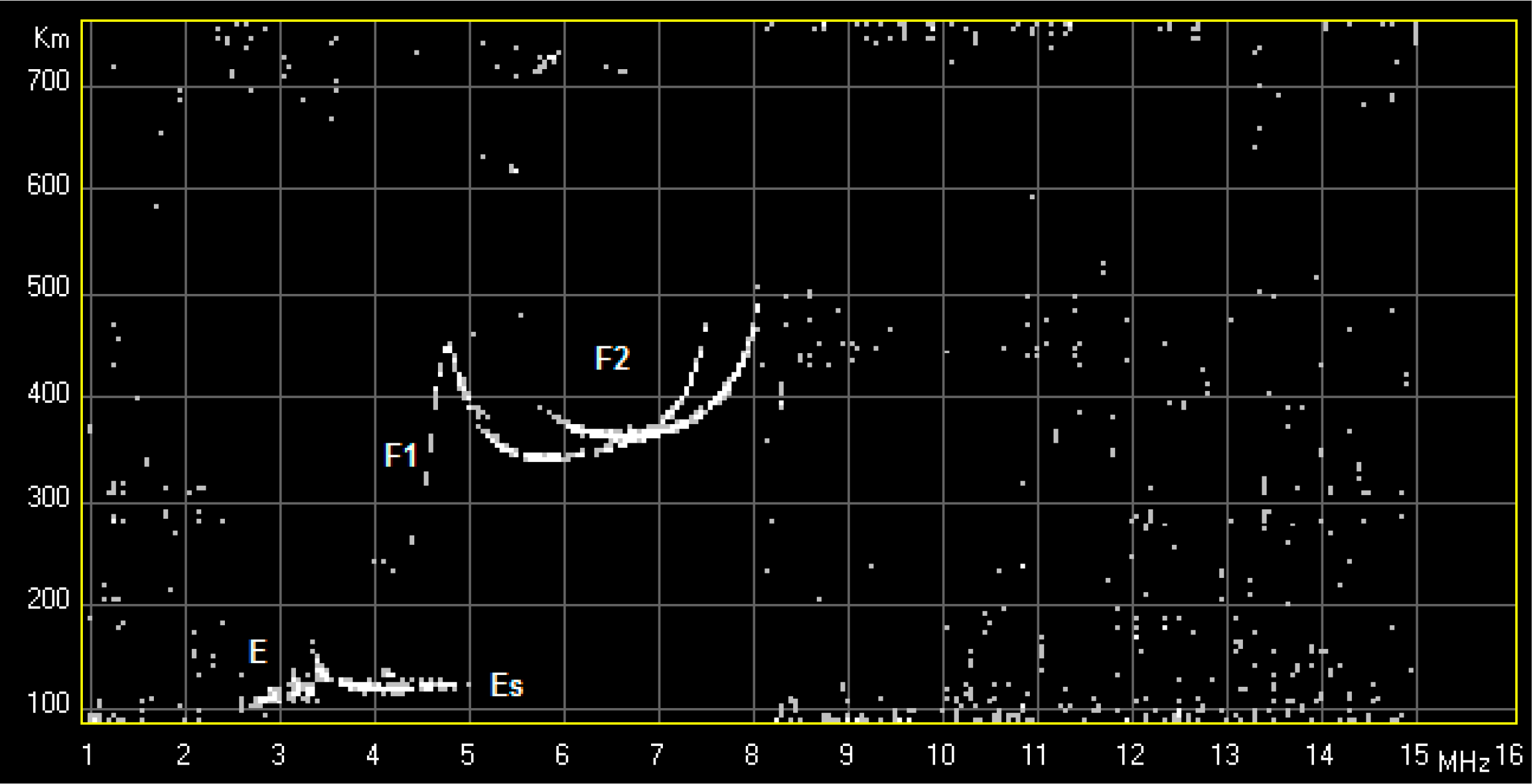
The VIS installed at the ASJI runs only when the station is attended, usually from December through early March, recording vertical incidence ionograms at 10 min sampling (see Figure 2). The ionograms are graphs representing the time-of-flight against transmitted radio frequency reflected in the ionosphere from which one extracts the ionospheric characteristics [18]. The measured characteristics are the lowest frequency observed in the ionogram (fmin), the critical frequencies of the ionospheric layers E, Es, F1 and F2 (foE, foEs, foF1 and foF2, respectively), the virtual (or group) heights of the ionospheric layers E, Es, F1 and F2 (h’E, h’Es, h’F1 and h’F2, respectively), and the maximum usable frequency for a single hop transmission at 3000 km reflected at the F2 layer (MUF(3000)F2). Note that the virtual heights (h’) give an estimation of the height at the bottom of the respective ionospheric layer and the critical frequencies (f0) are related to the maximum electron density (Nm) of the particular ionospheric layers by the following well known expression: , where density is expressed in m−3 and frequency in Hz. We refer the reader to [15] for more details.
2.3. HF Channel Parameters
Our analysis of the channel has been done both in a narrowband and wideband approach. The narrowband analysis focuses on channel availability and SNR computation. The channel availability means the probability of a link to reach a minimum SNR value and hence achieve a certain quality of service. According to [19], a minimum SNR value of 6 dB was specified to estimate the channel availability in a bandwidth of 10 Hz. As the probability of false alarm caused by noise and interferences is quite high when you measure the channel availability, several techniques to improve the reliability of the detection system have been developed [20].
The SNR is computed by comparing the received power measured during the tone intervals to the noise power measured during the idle periods.
The wideband analysis focuses in the calculation of the scattering function from the estimated channel impulse response. The composite multipath spread and Doppler spread parameters are also calculated as explained below.
Channel estimation was performed through a classical ML (maximum likelihood) based technique sending periodic Pseudo Noise (PN) waveforms with good cyclic cross-correlation characteristics. We used maximum-length shift-register sequences, or m-sequences for short [16]. Let PN[n] be the transmitted sequence of length Ne (in samples) and r[n] the received signal during the sounding interval. Then, the correlation of the received signal with a replica of the emitted sequence is carried out:
The channel matrix is calculated as:
From the scattering function the multipath power profile is calculated as:
Similarly, the Doppler power profile is obtained as:
We have also measured the absolute propagation time as a function of frequency, that is, the time it takes the wave to travel from LIV to Spain. This gives us some ideas about whether the wave has travelled along the standard path or some extraordinary paths are present. Finally, we have measured the Doppler frequency shift caused by the continuous movement of the reflective layers during the day, so we can measure the absolute speed of the layers.
3. System Description
The remote observatory in the ASJI is made of a geomagnetic and ionospheric sounding system and a transmission system that performs both the channel estimation and the transmission of data from the sounders.
3.1. Geomagnetic Recording System
Due to the wide amplitude and frequency ranges of the field sources monitored by observatories, highly sensitive and stable instruments (generally termed magnetometers) are operated in an environment free from artificial magnetic disturbance. Two sets of magnetometers are usually required: on the one hand, variometers are automatic instruments recording high-resolution, high-frequency variations of the Earth’s magnetic field; however, this feature is counter-balanced by the lack of long- or medium-term stability, e.g., against temperature or pillar movements; on the other hand, absolute instruments (whose measurements in theory do not depend on physical parameters other than the magnetic field itself) refer the recorded variations to the geographic reference frame.
Automatic recording is accomplished with diverse instrumentation based on different physical properties. The ones in use at LIV are based on fluxgates and proton precession magnetometers, whose technologies are summarized here:
- The fluxgate technology is based on the electric current induced in a coil submitted to both, the natural and a known artificial magnetic field in the presence of a magnetically susceptible core close to saturation. Three mutually orthogonal fluxgate bars can be used to refer vector variations, each determining the magnetic field projection along its axis. The fluxgate magnetometer at LIV (Figure 3) is a triaxial one; it is sampled at a rate of once per second and provides about 0.1 nT effective resolution.
- Proton precession magnetometers (PPM) are based on the intrinsic dipole magnetic moment of protons precessing around the ambient magnetic field, thus measuring the total magnitude F of the geomagnetic field with typical accuracies of 0.2 nT. When coils (usually two mutually perpendicular pairs of Helmholtz coils) are placed around them, a known current produces a known magnetic field that is superimposed to the natural one. Measurement of the resulting total field with the PPM allows determining variations of the declination and inclination angles. Two PPMs are used at LIV, which are sampled every ten seconds: one of them is a single scalar PPM to just measure F; the other is placed within two sets of Helmholtz coils, which produce a complete cycle of measurements including F, I and D every minute, constituting a variometer known as Proton Vector Magnetometer in δD/δI (or deltaD/deltaI) configuration.
Currently, there are two widely-used types of absolute instruments found in most geomagnetic observatories:
- The scalar PPM again, for measurements of the “total force”, F.
- The D/I fluxgate magnetometer, or D/I-flux. The fluxgate technology explained above is also used in this case, where the sensor is tightly coupled to the telescope of a theodolite. The angles thus measured are referred to previously determined geographic references, allowing the angles intrinsic to the magnetic field, D and I, be established. This instrument requires skilled manual operation, though some automated copies, known as AUTODIF, are already available for use [24]. Our short-term plans at LIV include deploying an automated D/I-flux, which would allow absolute measurements theoretically available during the whole year (i.e., including the unattended periods).
Data processing from both variometers and absolute instruments roughly entails (1) thorough detection of spurious records (e.g., spikes and artifacts) in the series; and (2) translation of automatically recorded vector component variations to their absolute level (see [25] and references therein).
Robust hardware has been designed to manage the acquisition of the variometers, both by the companies/institutes providing the instruments and by the technical staff at Ebre Observatory. We have almost doubled our control and logging systems to avoid data loss in case a hypothetical failure is produced during the unattended period. The control electronics is based on PIC 18F4550 and 16F877 microcontrollers managing the acquisition of our two PPM magnetometers. The first PIC is also used to control the triaxial fluxgate acquisition, with an Analog-to-Digital (A/D) converter to digitize its output. Two low-consumption (embedded) PCs are used to log the data, and a satellite transmission system is used to transfer the raw geomagnetic data to the corresponding INTERMAGNET GIN.
3.2. Ionospheric Sounding System
The ionospheric sounding system deployed at the ASJI is a VIS system, particularly the Advanced Ionospheric Sounder (AIS) developed by the Istituto Nazionale di Geofisica e Vulcanologia (INGV) of Rome, Italy. The main reasons to choose this system were the limited time of operation, low-cost and simple infrastructure and transport. The VIS might run only when the ASJI is attended, usually from December through early March, and only an inexpensive instrument was allowed for the proposal. The field available for installing research systems was very limited at that moment, being unrealistic to build an array of receiving antennas. The power supply of the ASJI was also limited, and a low consumption system was required. AIS accomplished all the above restrictions compared to other ionospheric systems available in the market. The authors of [26] provide details of the AIS sounder and [27] the signal processing techniques used. In summary, the main parts of the AIS are a frequency synthesizer, a code generator, a power amplifier and a delta type transmitting antenna into the transmission section; and a delta type receiving antenna, a radio receiver, an analog to digital converter and a digital signal processor into the receiving section. In addition, each section is controlled by a personal computer that also stores and displays data. AIS employs a 16 bit complementary phase code and exploits the advanced HF radar techniques, such as pulse compression and phase coherent integration. Figure 4 shows a detail of the transmitting and receiving antennas of the AIS deployed at the ASJI.
The AIS was upgraded during the surveys 2012–2013 and 2013–2014, with a new PC and operating system, as well as replacing the former PC ISA bus connection by an easier USB interface connection, adapting the system to current technology. Moreover, the system was upgraded with the Autoscala software [28], able to automatically estimate and scale ionospheric characteristics from ionograms and to estimate electron density profiles [29].
3.3. Transmission System
From the beginning, we discarded the use of commercial transceivers, as we wanted to analyze the channel in bandwidths greater than the 3 KHz standard bandwidth. Moreover, the system was conceived as a Software Defined Radio platform, so the carrier frequency, the bandwidth and the modulation can be changed by software.
The transmission system hardware of the channel sounder and the radio modem has been updated several times since the 2003/2004 survey. Three main Software Defined Radio (SDR) platforms have been installed in both the transmitter and the receiver. The first one, Sounding System for Antarctic Digital Communications (SANDICOM) was based on a HF radio controlled by a PC. The baseband signal was injected to the audio input of the transceiver, so the bandwidth was limited to 3 KHz and affected by the audio filter response [30].
During the 2005/2006 survey, a new software radio platform was developed using a Virtex FPGA and an external Digital Up/Down Converter responsible for mixing the RF signal to baseband, attenuating the adjacent channel interference and decimating the sampling frequency. This platform allowed us to test any bandwidth up to 15 KHz, and to cope with Signal-To-Interference Ratio (SIR) up to 80 dB [31]. However, the system had some relevant limitations. First, the maintenance was manual, which means that the daily configuration had to be changed connecting a laptop to the transmitter. The maintenance operations were done from 12:00 to 17:00 UTC, so neither sounding nor data transmissions were available during that period. As a consequence, the frequency range above 16 MHz, which propagate optimally during daytime, could not be observed. Moreover, both the GPS and the reference clock were medium quality devices, so the time and frequency accuracy was not very high. For these reasons, the absolute propagation time and the Doppler frequency shift could not be obtained.
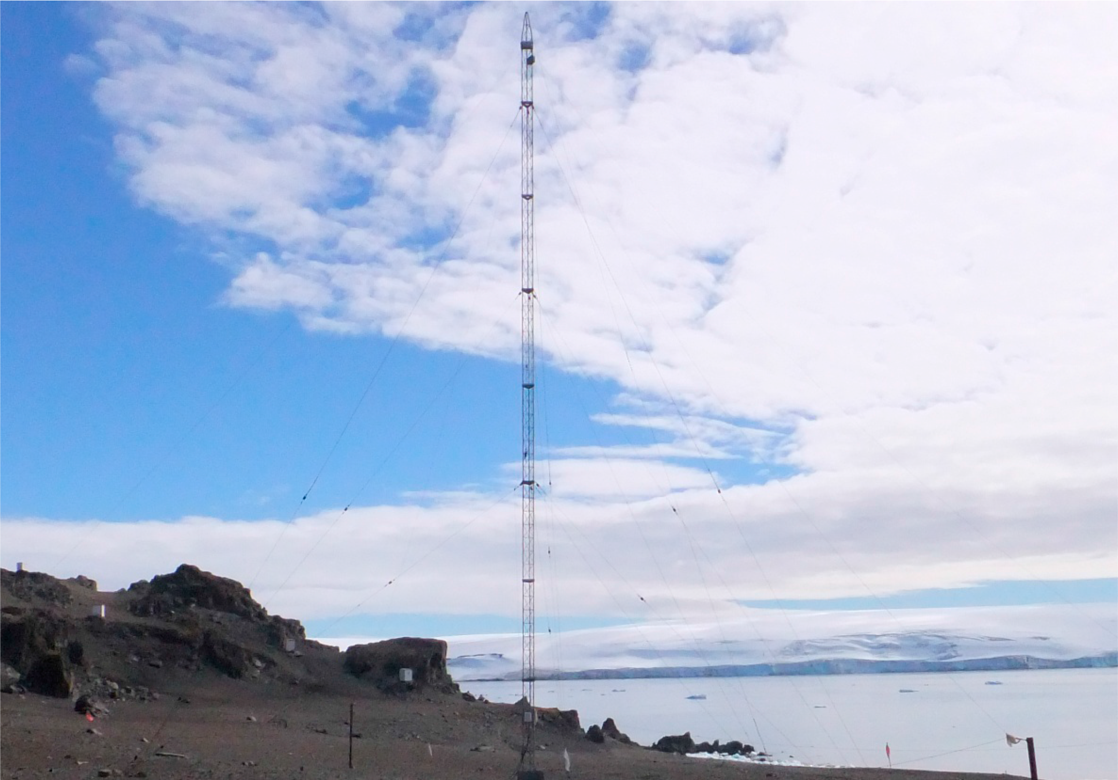
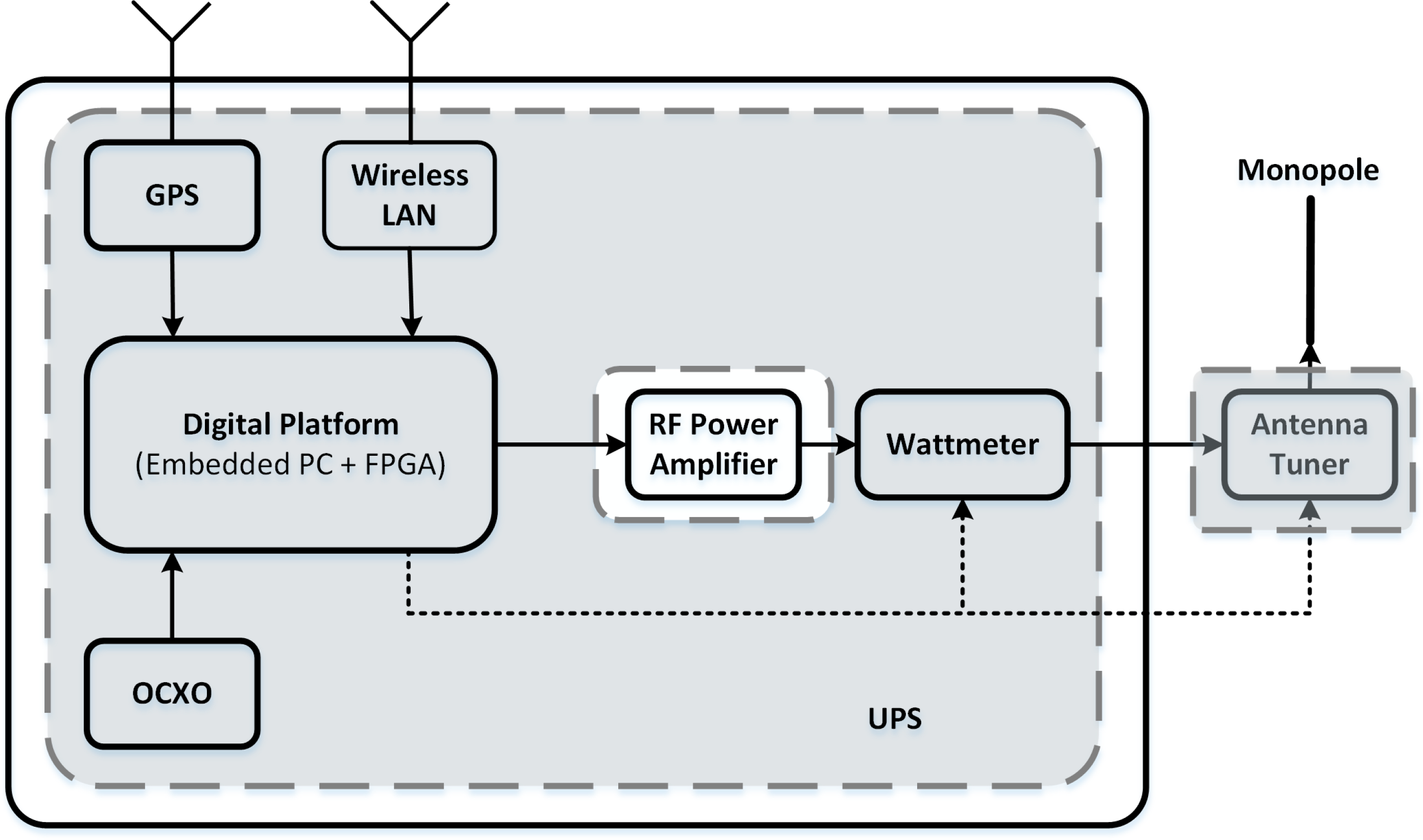
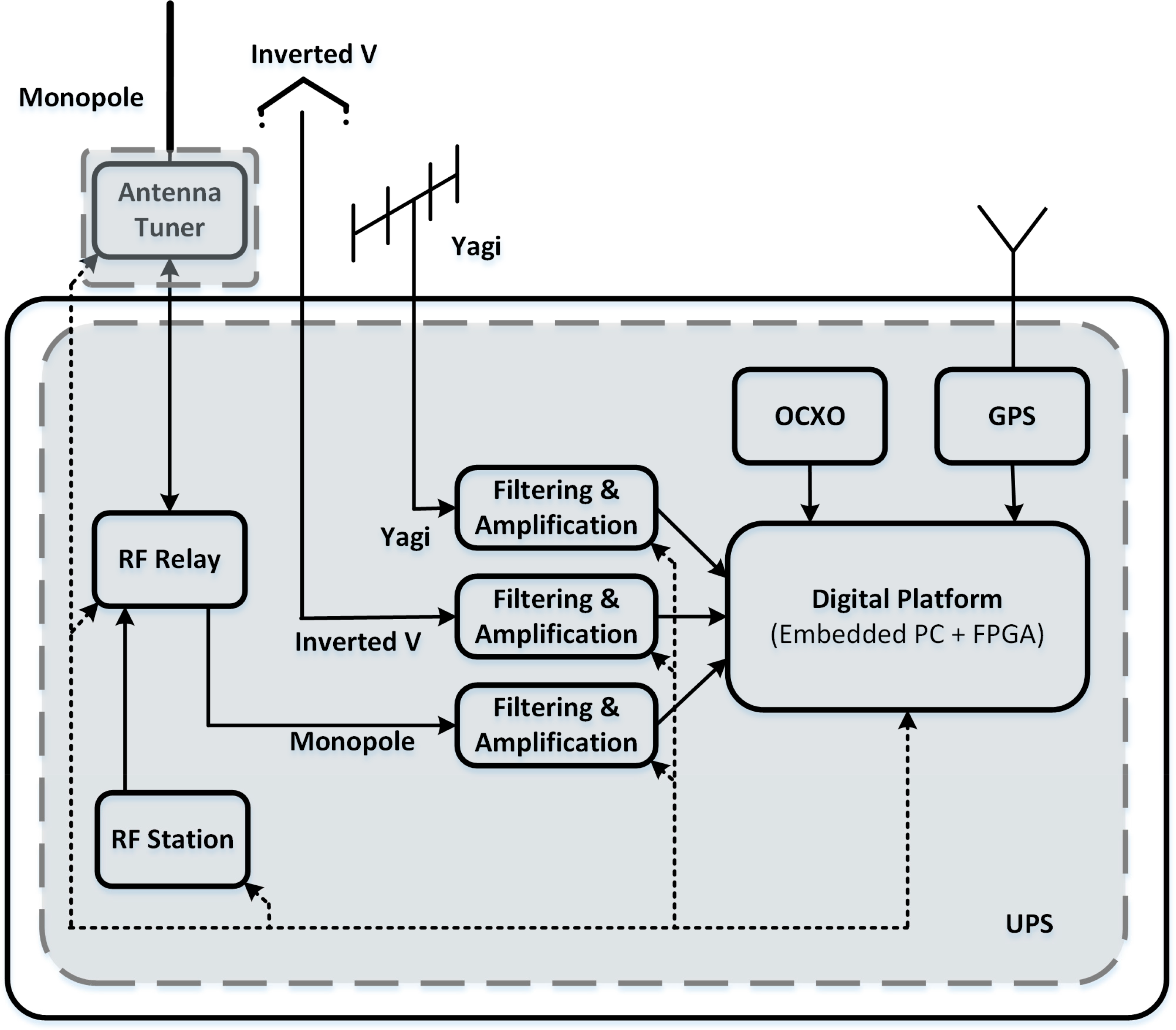
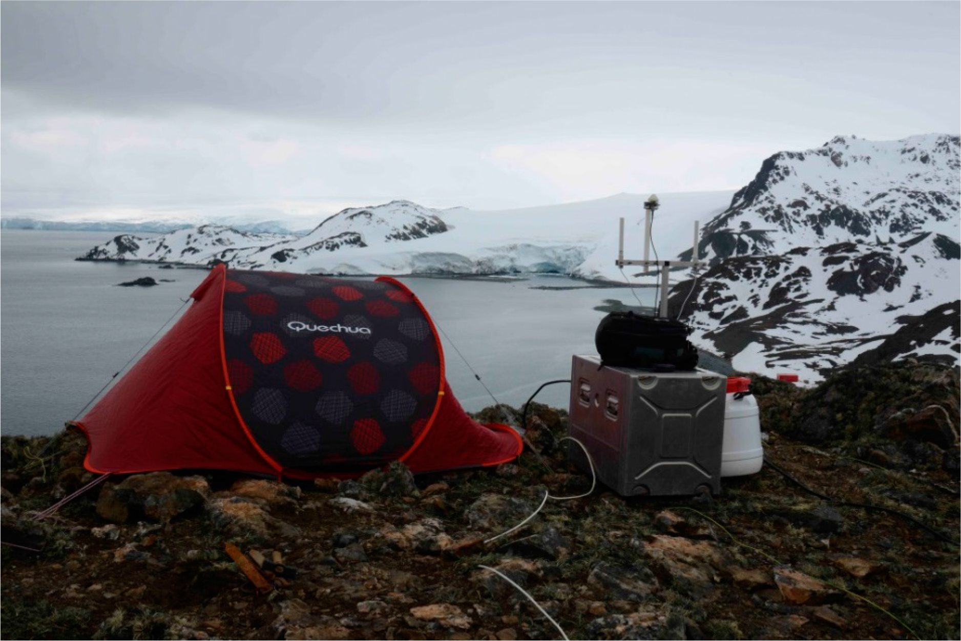
Finally, in the 2009/2010 survey, a third generation software radio platform was installed in both the ASJI and OE (see Figures 5 and 6). It is a weather resistant compact design installed near the antenna at the top of a hill close to ASJI (see Figure 7). The core of the system is a Virtex-4 XtremeDSP development platform from Xilinx with three FPGA that perform all the signal processing operations, included the up and down conversion. A new GPS unit with the Pulse per Second (PPS) signal increases the time synchronization accuracy (1 µs), making the measurement of the absolute propagation time of the wave possible. In order to improve the frequency synchronization accuracy, a 100 MHz Oven Controlled Crystal Oscillator (OCXO) was installed in both the transmitter and the receiver side. Moreover, the transmitter power amplifier can be switched off in case of severe impedance mismatch by means of a wattmeter that controls the forward and reverse transmitted power.
An embedded PC configures the transmitter and is remotely accessed by using a Wireless Local Area Network (WLAN) from the laboratory. Hence, the configuration is much faster and the system is able to work 24 h a day with an extended frequency range from 2 MHz to 30 MHz [20].
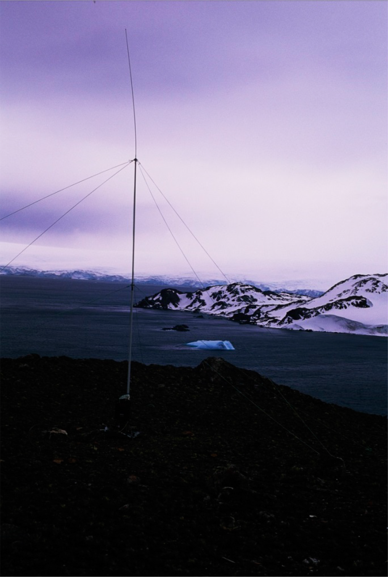
The transmitting antenna was a simple 7.5 m monopole with an antenna tuner able to operate in the whole HF band (see Figure 8). However, both the impedance matching and the radiation pattern were highly dependent on the goodness of the ground plane, thus, we installed a set of 32 radials that improved significantly the behavior in almost all the frequencies and the effective radiated power. As a result, the antenna tuner began to break more frequently, because the amount of backward power in case of mismatch and the voltage peaks were substantially higher. Then, we decided to develop a wattmeter with a directional coupler with a serial connection to the embedded PC. In case of severe mismatch (SWR > 2), the transmission was immediately aborted at that frequency and the failures were reduced considerably.
It is also worth mentioning that we had to face some electromagnetic compatibility issues. First, there were strong mutual interferences between our system and the vertical ionosonde. We had to define an accurate schedule of the tests in order to avoid simultaneous transmissions. Second, our transmitting antenna was radiating our own electronic system along the whole HF band, and both the PC and the FPGA board were halted several times. We had to shield the electronic boards carefully and place the transmitter a minimum of 40 m away from the antenna.
At the receiver side, we have also installed three synchronized software radio platforms to allow the simultaneous reception in a monopole, inverted-V and Yagi antenna. The monopole and the inverted-V are vertical and horizontal wideband antennas that allow polarization diversity tests in the whole HF band. We installed the radials for the monopole in the same way as we did in Livingston, and we mounted two lateral masts around the central mast in order to set the inverted-V as horizontal as possible. The directive radiation pattern of the Yagi antenna working around 14 MHz, reduces the amount of noise and interference coming from another directions and allows us to perform tests that need a higher SNR at the receiver.
4. Data Transmission
In this section, we describe the different tests that have been conducted to design the physical layer of the transmission system. The communication is simplex, i.e., the data from the sensor is only transmitted and no acknowledge is received, and the power transmission is kept very low for energy saving reasons. Moreover, it is not possible to install large antennas in the ASJI for environmental protection, so the final radiated power is very low. All this involves the design of an extremely robust reception system.
4.1. Tested Modulations
When transmitting data through a long-haul HF link, some important issues have to be taken into account. First of all, the best carrier frequency has to be chosen for the specific season and time of the day. Next, depending on the required bit rate, either a narrowband or wideband modulation scheme has to be designed. Our work is focused on wideband modulations specifically adapted to very low SNR scenarios. We have followed a similar evolution as the mobile communications schemes experienced from the second generation to the fourth generation systems.
The first proposal was a modified version of the classical Direct Sequence Spread Spectrum (DS-SS) scheme [16]. When using DS-SS techniques, spectrum is spread over a wider bandwidth, proportional to a pseudo noise (PN) sequence length L, being a robust modulation for rejecting high power narrowband interfering signals. The main drawback of the DS-SS proposal is the low spectral efficiency achieved when obtaining a good Bit Error Rate (BER) performance, since the bit rate available for a given bandwidth BW is about BW/L. However, there is no need for an accurate channel estimation and overhead synchronization, so it is a useful proposal for long-haul HF links. We have tested several bandwidths from 250 Hz to 20 KHz, as well as some PN sequence lengths from 31 to 127 chips [32].
After testing the basic DS-SS performance, we proposed a DS-SS signaling based physical layer able to achieve higher data rates while maintaining a good performance in low SNR communications [33]. DS-SS signaling consists on mapping m data bits into one of the M = 2m spreading codes. At the receiver, the transmitted bits are obtained by correlating the received time-frequency synchronized signal with the M spreading codes. Maximum correlation value determines the most probable transmitted spreading code, i.e., the most probable transmitted group of m bits. The implementation of M parallel correlators is feasible because of the low bandwidth of the baseband signal.
In the wireless communications world, the first spread spectrum standards have been replaced by several multicarrier standards. Orthogonal Frequency Division Multiplexing (OFDM) schemes emerged with Digital Video Broadcasting (DVB-T) and xDSL, and have been selected for the latest versions of the WiFi standards and LTE.
OFDM splits the input stream into several low bit rate subcarriers in such a way that the frequency selective channel becomes a flat channel for each subcarrier, making the equalization very simple. OFDM achieves higher throughputs in a fading channel than DS-SS [32], so it was the next proposal we tested in the Antarctic link. However, two important issues have to be carefully addressed. First, the frequency stability of the clocks in order to reduce the inter-carrier interference. Second, the non-constant envelope of the signal implies that some peaks arise above the mean value. This is the so-called Peak to Average Power Ratio (PAPR), which reduces the RF amplifier efficiency, since the mean power value of the amplifier has to be set to a lower value to avoid saturation and intermodulation products.
In order to design the OFDM physical layer, we tested the influence of several key parameters in the overall performance. Those parameters are summarized in Table 1.
Finally, we have also tested the Single Carrier modulation with Frequency Domain Equalization (SC-FDE) in order to explore the channel capacity without using spread spectrum techniques. The SC-FDE is a specific type of SC-FDMA (Single Carrier Frequency Division Multiple Access) for a single user, which is a near constant envelope version of OFDM that allows us to benefit from the maximum power of the amplifier [34].
4.2. Frame Organization
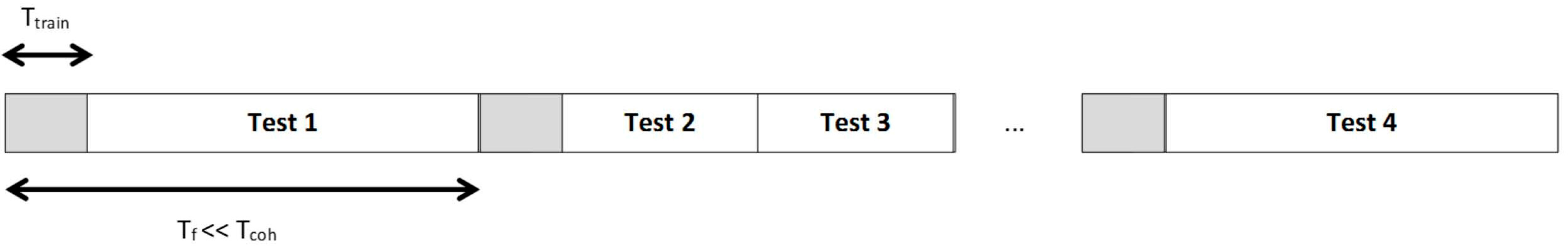
In the design of the modulations, synchronization has to be taken into account as a key process in the demodulation. The frame organization, while we perform tests to finish the design of the entire physical layer is the shown in Figure 9.
A synchronization sequence set (usually, three m sequences of length 2047 and oversampled with 10 samples per chip) is settled in the beginning of each data block [32]. The data block can contain either one test (with one bandwidth and symbol period) or several tests if these are shorter. However, the entire data block is mandatory to be shorter than a coherence time of the multipath ionospheric channel. The reason of this limitation is that with this criterion the receiver has information about the evolution of the channel performance. The bitrate depends on the modulation used, and varies from a range from 10 bps to 2 kbps. The dynamic margin of bitrates available are shown in Section 5.
5. Results
In this section, an overview of the results obtained during the last decade is presented. First, we review the historical series of both magnetic field and vertical and oblique ionospheric sounding, which cover, around, a complete solar cycle.
Next, we summarize the results of the modulation tests done both in multicarrier and spread spectrum techniques.
5.1. Historical Series
5.1.1. Magnetic Field
The 17 years of operation of the LIV geomagnetic observatory has yielded a valuable data series, with accurate datasets during the attended (summer) season, complying with all of the IAGA standards [17], and even most of the more restrictive INTERMAGNET standards [35] as far as accuracy, sampling rate, and data processing requirements are concerned. The winter seasons have been, however, more controversial. Interruptions due to power loss from the base, or incidences in the observatory hardware and software have sometimes left the station partially or totally disabled for several months in a row. However, these relatively few gaps have not avoided a characterization of the largest peak amplitudes, which reached a drop of around 1300 nT in the magnetic field strength during the main phase of a severe magnetic storm [36], or the behavior of the quiet-day variations [2]. As for the extreme expected values, unfortunately the Halloween storm (29–31 October 2003), one of the major space weather historical events, coincided with one of those unattended periods in which we lost data (in that occasion it was due to the breakage of the wind generators that, along with some solar panels, were supplying power during the winter), thus, although rare, even more extreme scenarios than the above mentioned are possible. As for the regular daily variation, the largest amplitudes occur, as expected, during the summer and the smallest in winter, with the typical patterns in each component for a station located south of the southern hemisphere current focus but still away from the auroral region. A clear dependence of the Sq amplitude on solar activity was also found.
Other results from LIV data concern instrumental aspects, which, although strictly speaking are only valid for the instruments operating at LIV, other observatories with similar equipment can benefit from. On one hand, a summarized description of the principles and operation of the δD/δI variometer was given in [37], while an assessment of their accuracy and time resolution given the assumed approximations, together with a critical examination of their potential sources of error, can be found in [38]. Further on, once the observatory instrumentation was upgraded with the addition of the triaxial fluxgate magnetometer and new sampling hardware and data logging software (as described in [36]), simultaneous data comparisons with the old δD/δI variometer helped to assess the temperature sensitivity of both [39,40]. It has been revealed that both instruments are sensitive to temperature variations, but in a dynamic way, and with a different response for each magnetic element. In general, results show a somewhat higher temperature sensitivity of the large size δD/δI coils than that of the fluxgate variometer. On the other hand, an assessment of the performance of the D/I-flux instrument in use at LIV, and an analysis of the sources of uncertainty that in general this kind of instruments present can be found in [41]. This latter article reveals that, although the D/I-flux has become the international standard to undertake absolute measurements of the angular elements in every geomagnetic observatory, its accuracy is limited by a series of effects, and a list of recommendations for the reduction of errors is given as well.
For what concerns data processing aspects, LIV data (among others) have been used in [42] to investigate the impact of fundamental minute-data loss in the computation of the observatory hourly mean values of the geomagnetic field, where limits in the number of missing data are recommended to produce representative values.
Finally, along with those mentioned in the introduction, LIV data has been used to support for several geophysical studies. In a local or regional framework, they served as a base station for the reduction of magnetic surveys [43–45], for the synthesis and updates of Antarctic reference field models [46–49], or for the characterization of the variability of the ionospheric currents responsible for the Sq variation in the South American-Antarctic Peninsula region [2]. They, of course, contributed for the generation of surely all global models produced after LIV data became available which used geomagnetic observatory data to characterize the behavior of the geomagnetic field and its secular variation (SV) at the Earth’s surface, but also for downward extrapolations to infer core flow right beneath the core mantle boundary, which are critical for understanding the dynamical processes in the Earth’s core. There could be dozens of them. Reviews of this kind of models can be found in [50] or [51]. It is worth mentioning, the model of the SV for the 1995–2000 epoch of [52], in which LIV hourly mean values are particularly used to show the procedure used to correct their selection of nighttime values for annual variations of the magnetospheric contribution. LIV data (among others) have also been used to assess the validity of an improvement made in the National Center of Atmospheric Reasearch (NCAR) Thermosphere-Ionosphere Electrodynamics General Circulation Model (TIEGCM), where satellite geomagnetic field-aligned current data were used to feed the model [53].
5.1.2. Vertical Ionospheric Sounding
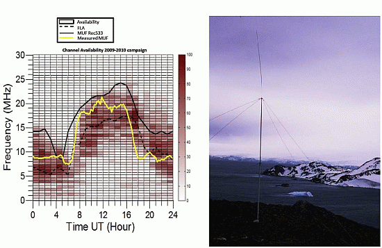
The typical pattern of the summer behavior of the ionospheric F2 characteristics and of their variability was evaluated for different Spanish Antarctic surveys, and the differences of the above patterns from survey to survey were related to the different solar activity [54]. Such a pattern at mid-high latitudes of the ASJI was also compared with the summer behavior at other mid-latitude stations and it was noticed a larger post-sunset electron density enhancement at the ASJI than that recorded in other regions. The significant decrease of the foF2 and their strong uplift of the F2 layer as observed by the significant increase in the virtual height, h’F2, for the geomagnetically disturbed period of 18 February 2005, was also investigated and explained in terms of a response of the ionosphere to the geomagnetic storms [55,56]. In addition, the data recorded with the AIS VIS, especially MUF(3000)F2, have been correlated with data extracted from the HF radio link established between the ASJI and Spain [57]. This HF radio link was used as multi-hop Oblique Ionospheric Sounder, OIS. In [57], Vilella et al. have shown that the frequencies with largest availability of the HF radio link (FLA) correlate reasonably well with the MUF(3000)F2 recorded by VIS placed at the receiver site (40.8°N, 0.5°E) (see Figure 10, left) and that frequencies of OIS delivered at the receiver being larger than the MUF(3000)F2 recorded by VIS suffer a significant drop of power. The left plot of Figure 9 also shows the maximum usable frequency obtained by the Rec 533 model (MUF Rec 533) which is defined as the highest frequency for which an ionospheric communication path is predicted on 50% of the days of the month [58]. The above studies obtained with the ionospheric sensors installed at the remote region of the ASJI for surveys July 2006 have been extended for three consecutive surveys (October 2009, November 2010, and December 2011) with different solar activity levels observing the effect of increasing the solar activity.
Other results obtained by the team show significant correlation of the MUF(3000)F2 recorded by VIS with signal to noise ratio of the HF radio link established between the ASJI and Spain (SNR) as can be shown in Figure 10, right. This fact jointly with the aforementioned results presented in [57] motivates us to future development of models for predicting the best frequencies for establishing the HF radio link between the ASJI and Spain. Moreover, we found additional correlation between observations by the OIS and by VIS at the receiving site. Thanks to the upgrade of the OIS with more accurate clocks and better GPS for synchronization, it was possible to analyze the time of flight and the Doppler shift and to notice that the Doppler shift suffered for the radio link between ASJI and Spain correlates with the vertical drift velocity of the ionospheric F region over the receiving site in Spain (see Figure 11). Altadill et al. [59] show details on the measurements of the F-region vertical drift velocity and the results of its daily pattern.
5.1.3. Oblique Ionospheric Sounding
In this section we synthesize the results for both narrowband and wideband oblique sounding. Exhaustive results can be found in [19,20]. We note that the oblique ionospheric sounding study provided results in terms of (i) availability of the channel, crucial to improve transmission; and (ii) multipath and Doppler spread, being the multipath spread a limit for symbol period and the evaluation of coherence time using the Doppler spread as a reference to build the frame data blocks.
Only the results for the best transmission hours are shown in Table 2. The analysis is based on the SNR measure, so conclusions shall be taken with caution. The best transmissions are obtained from 00 UTC to 04 UTC around 9 MHz, and at 21 UTC at higher bands, around 15 MHz. Nowadays we still use this sounding to settle the first transmission frequencies, being modified depending on their performance after each sounding campaign analysis.
5.2. Tested Modulations
We have tested several modulation techniques for low-power simplex remote sensors communications in the HF band over the last decade. The system is currently transmitting the data from the sensors of the Ebre Observatory in the ASJI, but it also could be used to transmit the data from any other remote sensor.
When designing a communication system, there is always a trade-off between robustness and bit-rate. If robustness and Bit Error Rate (BER) are main factor to be optimized, spread spectrum techniques [16] are the choice then. On the other hand, if bitrate and spectral efficiency are the key issue, then OFDM and Single Carrier [16] have to be tested.
A synthesis of the BER and bitrate results are shown, but more detailed results for the entire modulation tests can be found in the following works: (i) comparison between DS-SS and OFDM in [32] (see Table 3); (ii) comparison between DS signaling and quadriphase, in order to increase the bitrate of DS-SS without worsening the BER in [33] (see Table 4); (iii) comparison between several types of Single Carrier in [60] (see Table 5) .
In Table 3, BER results for the comparison of DS-SS and OFDM are shown. Very low bitrate was tested, because the objective of the comparison was to find a modulation (or a set of modulations) that achieved BER=0 most of the time. The system can assume higher BER using channel coding, but we intended to determine the lower limit, and then tried to increase the bitrate when this limit was reached. To validate the best modulations, we focused the BER value with a probability of 30% in the cumulative density function of the proper BER. This measure means that the 30% of the best-performed tests results obtain the noted value (see Table 3) as their worst case.
After these first tests, the modulation search was refined. Table 4 shows the results for the comparison of signaling and quasi-quadriphase, two evolution techniques based on DS-SS. Both use a family of Gold PN sequences [61] to address n data for each sent sequence, where the PN sequence is length 2n − 1. As shown in Table 4, bitrate is clearly improved by setting a symbol time that performed good results in the comparison of Table 3, and increasing the PN sequence length and reducing the number of samples per chip. Stability and robustness are the fundamental goals of these two DS-SS variations.
Finally, Table 5 shows the proof of principle of a Single Carrier proposal for the ionospheric channel. The goal of this proposal is to increase the bitrate significantly, reaching one order of magnitude higher than the shown in Table 4. Despite the bitrate improval, the BER results shown are not as good as the ones for signaling and quadriphase.
Nowadays, the research group is working in the evolution of Single Carrier and also in increasing the bandwidth of signaling and quadriphase transmissions to improve their BER and bitrate results.
6. Conclusions
In this paper, the main results of the Remote Geophysical Observatory in the Spanish Antarctic Station Juan Carlos I in Livingston Island over the last ten years have been summarized.
The Livingston Island geomagnetic observatory continuously records all components of the Earth’s magnetic field since December 1996. As a natural result of the evolving standards in geomagnetic observatory practice, the LIV geomagnetic observatory has undergone continuous upgrade during such more than 17 years of history, the most remarkable one including a three-axis fluxgate sensor enabling an accurate 1 Hz sampling rate. Data during these years have been thoroughly processed and published. Since it is deployed at a remote site, which is only manned during restricted periods of time (summer), those records are subject to uncertainties for periods with no absolute measurements, thus assumptions have been made concerning the baselines evolution during those periods. The “definitive” data of LIV have been used by our and other worldwide research teams, having significantly contributed to research work in a number of fields such as plate tectonics, global and regional main field modeling, or to understand the mechanisms of the local and regional geomagnetic field variations in general, and Sq characterization, in particular. Instrumental behavior under severe climate conditions has also been a necessary topic of research. As a consequence of the contemporaneous evolution in the observation standards, we are now facing a challenging upgrade that would consist in the setup of an automatic absolute instrument, along with specific hardware to allow an enhanced accuracy and sampling rate outcome to yield filtered 1-s data.
The ionospheric instruments installed at the ASJI (AIS) made possible ionospheric research at that subauroral remote region. The climatology and variability of the ionospheric characteristics have been studied from survey to survey. Moreover, it was possible investigating the ionospheric effects caused by space weather events at that remote region. Data recorded there served also to validate prediction models of ionospheric characteristics. Thanks also to the HF radio link established between the ASJI and Spain used as a multi-hop OIS, several correlations between observations with OIS and VIS; the latter recorded at stations located along the radio path, including VIS stations at the emitter and receiver sites. These results show that relevant information (e.g., maximum received frequency, FLA, Doppler shift) of the very long range radio links from ASJI to Spain can be estimated with an appropriate modeling using VIS data along the path, but especially at the receiving site. The results developed by the team under the framework the Antarctic Spanish projects show the potential of this infrastructure for ionospheric monitoring and research purposes at subauroral regions.
As far the vertical sounding is concerned, we have the historical series of the key parameters of the channel along more than ten years. The parameters are the delay spread and the Doppler spread and shift as a function of the frequency and the time, as well as the SNR for every frequency and the amount of interference. This database gives us a deep knowledge of the channel and is a great support to design the modulation scheme, the error correcting codes, the interleaver and the rest of parameters that define a complete physical layer.
We have also tested some types of modulations that fit well to a slow fading multipath channel. We developed some variations of the classical Direct Sequence Spread Spectrum that are highly robust in low SNR scenarios at the expense of the low bit-rate. The spread spectrum approach does not interfere with other signals in the same band, and it is a good approach for sensors with low data rate. Then, we also tested the multicarrier approach (OFDM) in order to increase the bit-rate using some parallel orthogonal subcarriers at the same time. In practice, OFDM does not ensure a greater capacity in our link, because the available transmitting power is very low and we could use a small amount of subcarriers. Moreover, the effective mean power is even lower due to the PAPR problem, and the need of a linear amplifier increases the cost of the system. Finally, we have tested the Single Carrier approach with Frequency Domain Equalization. The increase of bit-rate is highly remarkable, at the expense of a poorer BER, which can be corrected with the proper codes. Therefore, it is a good candidate for remote sensors that need a higher throughput.
Although the best modulations have been already determined, the complete definition of the physical layer, that is, the structure of the frame, the synchronization methods, the coding and interleaving schemes, have not been totally defined yet. At this moment, the hardware design is completed, but the definition of the complete physical layer for the communication of remote sensors in HF is about to be completed.
Acknowledgments
This research has been supported by the Spanish Projects CTM2010-21312-C03, CTM2009-13843-C02, CGL2006-12437-C02 and REN2003-08376-C02. In addition to the authors of this paper, the following people have been part of the research groups of these projects: Ahmed Ads, Luis Felipe Alberca, Emil Marcel Apostolov, Ricard Aquilué, Raúl Bardají, Cesidio Bianchi, Estefania Blanch, Josep Oriol Cardús, Oscar Cid, Juan José Curto, Angelo De Santis, Marc Deumal, Luis Ricardo Gaya-Piqué, Simó Graells, Ismael Gutierrez, Marcos Hervás, Miguel Ibáñez, Joan Mauricio, David Miralles, Pere Quintana, Joan Ramon Regué, Xavier Rosell, Martí Salvador, Albert Miquel Sanchez, Ernest Sanclement, José Germán Solé, Arantza Ugalde, Carles Vilella. John C. Riddick, retired from the Global Seismology and Geomagnetism Group of the British Geological Survey, deserves special mention. The installation and upgrading of the geomagnetic observatory system would have been impossible without him.
Author Contributions
Joan Lluis Pijoan has been the principal investigator during the whole project in the part of channel sounding and testing of advanced modulations. He had the idea of writing a review paper and wrote the introductory chapter and the conclusions concerning the HF transmission system. David Altadill has been the principal investigator during some periods of the project. He has conducted the ionospheric research throughout the project and wrote the parts of the paper related to VIS and its correlations with OIS. Joan Miquel Torta has been the principal investigator during some periods of the project in the part of geomagnetic and ionospheric sounding. He deployed and installed the first geomagnetic observatory system, maintained it during three of the surveys and processed its data for several years. He wrote parts of the paper concerning the geomagnetic observatory. Rosa Ma Alsina-Pagès is behind the modulation data tests and wrote the modulation comparison study in this paper. She is also leading the design of the physical layer for the transmisson system. Santiago Marsal has been in charge of the technical questions concerning the geomagnetic station for the last twelve years; in particular, he has developed software to process its data, has contributed to designing the upgrade of the observatory, has participated in eight Antarctic surveys, and has contributed in writing the geomagnetism part of the present paper. David Badia installed the transmission system in Antarctica, installed the receiver system in Spain and reviewed the paper.
Conflicts of Interest
The authors declare no conflict of interest.
References
- Maldonado, A.; Balanyá, J.C.; Barnolas, A.; Galindo-Zaldívar, J.; Hernández, J.R.; Jabaloy, A.; Livermore, R.A.; Martínez-Martínez, J.M.; Rodríguez-Fernández, J.; Sanz de Galdeano, C.; et al. Tectonics of an extinct ridge-transform intersection, Drake Passage (Antarctica). Mar. Geophys. Res 2000, 21, 43–68. [Google Scholar]
- Torta, J.M.; Marsal, S.; Curto, J.J.; Gaya-Piqué, L.R. Behaviour of the quiet day geomagnetic variation at Livingston Island and variability of the Sq focus position in the South American-Antarctic Peninsula region. Earth Planets Space 2010, 62, 297–307. [Google Scholar]
- Finlay, C.C.; Maus, S.; Beggan, C.D.; Bondar, T.N.; Chambodut, A.; Chernova, T.A.; Chulliat, A.; Golovkov, V.P.; Hamilton, B.; Hamoudi, M.; et al. (Participating members of the IAGA, WG V-MOD). International geomagnetic reference field: The eleventh generation. Geophys. J. Int 2010. [Google Scholar] [CrossRef]
- Maus, S. An ellipsoidal harmonic representation of Earth’s lithospheric magnetic field to degree and order 720. Geochem. Geophys. Geosyst 2010. [Google Scholar] [CrossRef]
- Semenov, A.; Kuvshinov, A. Global 3-D imaging of mantle electrical conductivity based on inversion of observatory C-responses-II. Data analysis and results. Geophys. J. Int 2012. [Google Scholar] [CrossRef]
- Richmond, A.D. Assimilative mapping of atmospheric electrodynamics. Adv. Space Res. 1992. [Google Scholar] [CrossRef]
- Blanch, E.; Marsal, S.; Segarra, A.; Torta, J.M.; Altadill, D.; Curto, J.J. Space weather effects on Earth’s environment associated to the 24–25 October 2011 geomagnetic storm. Space Weath 2013, 11, 153–168. [Google Scholar]
- Torta, J.M.; Serrano, L.; Regué, J.R.; Sánchez, A.M.; Roldán, E. Geomagnetically induced currents in a power grid of northeastern Spain. Space Weath 2012. [Google Scholar] [CrossRef]
- Reinisch, B.W. Ionosonde. In Upper Atmosphere; Dieminger, W., Hartmann, G.K., Leitinger, R., Eds.; Springer: Berlin, Germany, 1996; pp. 370–381. [Google Scholar]
- Reinisch, B.W.; Galkin, I.A.; Khmyrov, G.M.; Kozlov, A.V.; Bibl, K.; Lisysyan, I.A.; Cheney, G.P.; Huang, X.; Kitrosser, D.F.; Paznukhov, V.V.; et al. New Digisonde for research and monitoring applications. Radio Sci 2009. [Google Scholar] [CrossRef]
- National Oceanic and Atmospheric Administration. Available online: http://www.osd.noaa.gov/GOES/GOES-NOP_Brochure.pdf (accessed on 10 May 2014).
- NOAA’s Satellite and Information Service (NESDIS). Available online: http://www.nesdis.noaa.gov/ (accessed on 10 May 2014).
- National Oceanic and Atmospheric Administration. Available online: http://www.osd.noaa.gov/Spacecraft%20Systems/Pollar_Orbiting_Sat/NOAA_N_Prime/NOAA_NP_Booklet.pdf (accessed on 10 May 2014).
- ARGOS-Worldwide Tracking and Environmental Monitoring by Satellite. Available online: http://www.argos-system.org/ (accessed on 10 May 2014).
- Davies, K. Ionospheric Radio; Peter Peregrinus: London, UK, 1990. [Google Scholar]
- Proakis, J. Digital Communications, 4th ed; McGraw Hill: Boston, MA, USA, 2000. [Google Scholar]
- Jankowski, J.; Sucksdorff, C. IAGA Guide for Magnetic Measurements and Observatory Practice; International Association of Geomagnetism and Aeronomy: Warsaw, Poland, 1996. [Google Scholar]
- World Data Center A for Solar-Terrestrial Physics, U.R.S.I. Handbook of Ionogram Interpretation and Reduction; Report UAG-23; Piggott, W.R., Rawer, K., Eds.; National Oceanic and Atmospheric Administration (NOAA): Asheville, NC, USA, 1972.
- Vilella, C.; Miralles, D.; Pijoan, J.L. An Antarctica-to-Spain HF ionospheric radio link: Sounding results. Radio Sci 2008. [Google Scholar] [CrossRef]
- Ads, A.G.; Bergadà, P.; Vilella, C.; Regué, J.R.; Pijoan, J.L.; Bardají, R.; Mauricio, J. A comprehensive sounding of the ionospheric HF radio link from Antarctica to Spain. Radio Sci 2012. [Google Scholar] [CrossRef]
- Angling, M.J.; Davies, N.C. An assessment of a new ionospheric channel model driven by measurements of multipath and Doppler spread. Proceedings of the 1999 IEEE Colloquium on Frequency Selection and Management Techniques for HF Communications, London, UK, 29–30 March 1999.
- Warrington, E.M.; Stocker, A.J. Measurements of the Doppler and multipath spread of the HF signals received over a path oriented along the midlatitude trough. Radio Sci 2003, 38. [Google Scholar] [CrossRef]
- Nissen, C.A.; Bello, P.A. Measured channel parameters for the disturbed wide-bandwidth HF channel. Radio Sci 2003. [Google Scholar] [CrossRef]
- Rasson, J.; Gonsette, A. The Mark II Automatic DIFlux. Data Sci. J. 2011, 10, IAGA169–IAGA173. [Google Scholar]
- Marsal, S.; Torta, J.M.; Solé, J.G.; Segarra, A.; Cid, O.; Ibáñez, M.; Altadill, D. Livingston Island Geomagnetic Observations 2012 and 2012–2013 Survey. Available online: http://www.obsebre.es/images/oeb/pdfs/es/BoletinesMagnetismo/livingston_2012.pdf (accessed on 12 February 2014).
- Zuccheretti, E.; Bianchi, C.; Sciacca, U.; Tutone, G.; Arokiasamy, J. The new AIS-INGV digital ionosonde. Ann. Geophys 2003, 46, 647–659. [Google Scholar]
- Bianchi, C.; Sciacca, U.; Zirizzotti, A.; Zuccheretti, E.; Baskaradas, J.A. Signal processing techniques for phase-coded HF-VHF radars. Ann. Geophys 2003, 46, 697–705. [Google Scholar]
- Pezzopane, M.; Scotto, C. The INGV software for the automatic scaling of foF 2 and MUF (3000)F 2 from ionograms: A performance comparison with ARTIST 4.01 from Rome data. J. Atmos. Sol.-Terr. Phys. 2005, 67, 1063–1073. [Google Scholar]
- Scotto, C. Electron density profile calculation technique for Autoscala ionogram analysis. Adv. Space Res 2009. [Google Scholar] [CrossRef]
- Vilella, C.; Miralles, D.; Socoró, J.C.; Pijoan, J.L.; Aquilué, R. A new sounding system for HF digital communications from Antarctica. Proceedings of the International Symposium on Antennas and Propagation, Seoul, South Korea, 3–5 August 2005; pp. 419–422.
- Vilella, C.; Bergadà, P.; Deumal, M.; Pijoan, J.L.; Aquilué, R. Transceiver architecture and Digital Down Converter design for long distance, low power HF ionospheric links. Proceedings of the Ionospheric Radio Systems and Techniques, London, UK, 18–21 July 2006; pp. 95–99.
- Bergadà, P.; Alsina-Pagès, R.M.; Pijoan, J.L.; Salvador, M.; Regué, J.R.; Badia, D.; Graells, S. Digital transmission techniques for a long haul HF link: DS-SS vs. OFDM. Radio Sci 2014. [Google Scholar] [CrossRef]
- Alsina-Pagès, R.M.; Salvador, M.; Hervás, M.; Bergadà, P.; Pijoan, J.L.; Badia, D. Spread spectrum high performance techniques for a long haul HF link. IET Commun 2014. submitted. [Google Scholar]
- Myung, H.G.; Goodman, D.J. Single carrier FDMA. In A New Air Interface for Long Term Evolution; John Wiley & Sons: New York, NY, USA, 2008; pp. 37–59. [Google Scholar]
- INTERMAGNET Technical Reference Manual, Version 4.6, Available online: http://www.intermagnet.org/publications/intermag_4-6.pdf (accessed on 12 February 2014).
- Torta, J.M.; Marsal, S.; Riddick, J.C.; Vilella, C.; Altadill, D.; Blanch, E.; Cid, O.; Curto, J.J.; de Santis, A.; Gaya-Piqué, L.R.; et al. An example of operation for a partly manned Antarctic geomagnetic observatory and the development of a radio link for data transmission. Ann. Geophys 2009, 52, 45–56. [Google Scholar]
- Torta, J.M.; Gaya-Piqué, L.R.; Riddick, J.C.; Turbitt, C.W. A Partly manned geomagnetic observatory in Antarctica provides a reliable data set. Contrib. Geophys. Geodesy Geophys. Inst. Slov. Acad. Sci 2001, 31, 225–230. [Google Scholar]
- Marsal, S.; Torta, J.M.; Riddick, J.C. An assessment of the BGS δDδI vector magnetometer. Publs. Inst. Geophys. Pol. Acad. Sci 2007, 99, 158–165. [Google Scholar]
- Marsal, S.; Curto, J.J.; Riddick, J.C.; Torta, J.M.; Cid, O.; Ibañez, M. Livingston Island observatory upgrade: First results. Proceedings of the XIIIth IAGA Workshop on Geomagnetic Observatory Instruments, Data Acquisition, and Processing, Boulder and Golden, CO, USA, 9–18 June 2008.
- Marsal, S.; Torta, J.M.; Curto, J.J. Temperature sensitivity of variometers: Lessons learnt from Livingston Island geomagnetic observatory. Proceedings of the XVth IAGA Workshop on Geomagnetic Observatory, Instruments, Data Acquisition and Processing, Cádiz, Spain, 4–14 June 2012.
- Marsal, S.; Torta, J.M. An evaluation of the uncertainty associated with the measurement of the geomagnetic field with a D/I fluxgate theodolite. Measur. Sci. Technol 2007, 18. [Google Scholar] [CrossRef]
- Marsal, S.; Curto, J.J. A new approach to the hourly mean computation problem when dealing with missing data. Earth Planets Space 2009, 61, 945–956. [Google Scholar]
- Livermore, R.A.; Balanyá, J.C; Maldonado, A.; Martínez-Martínez, J.M.; Rodríguez-Fernández, J.; Sanz de Galdeano, C.; Galindo-Zaldívar, J.; Jabaloy, A.; Barnolas, A.; Somoza, L.; et al. Autopsy on a dead spreading center: The Phoenix Ridge, Drake Passage, Antarctica. Geology 2000, 28, 607–610. [Google Scholar]
- Catalán, M.; Agudo, L.M.; Muñoz, A. Geomagnetic secular variation of Bransfield Strait (Western Antarctica) from analysis of marine crossover data. Geophys. J. Int 2006, 165, 73–86. [Google Scholar]
- Catalán, M.; Galindo-Zaldivar, J.; Martín Davila, J.; Martos, Y.M.; Maldonado, A.; Gambôa, L.; Schreider, A.A. Initial stages of oceanic spreading in the Bransfield Rift from magnetic and gravity data analysis. Tectonophysics 2013, 585, 102–112. [Google Scholar]
- Torta, J.M.; De Santis, A.; Chiappini, M.; von Frese, R.R.B. A model of the secular change of the geomagnetic field for Antarctica. Tectonophysics 2002, 347, 179–187. [Google Scholar]
- De Santis, A.; Torta, J.M.; Gaya-Piqué, L.R. The first Antarctic geomagnetic Reference Model (ARM). Geophys. Res. Lett 2002, 29. [Google Scholar] [CrossRef]
- Gaya-Piqué, L.R.; Ravat, D.; de Santis, A.; Torta, J.M. New model alternatives for improving the representation of the core magnetic field of Antarctica. Antarct. Sci 2006, 18, 101–109. [Google Scholar]
- Tozzi, R.; De Santis, A.; Gaya-Piqué, L.R. Antarctic geomagnetic reference model updated to 2010 and provisionally to 2012. Tectonophysics 2013, 585, 13–25. [Google Scholar]
- Hulot, G.; Sabaka, T.J.; Olsen, N. The present field. In Treatise on Geophysics, Geomagnetism; Kono, M., Ed.; Elsevier: Amsterdam, The Netherlands, 2007; Volume 5, pp. 33–75. [Google Scholar]
- Lesur, V.; Olsen, N.; Thomson, A. Geomagnetic core field models in the satellite era. In Geomagnetic Observations and Models, IAGA Special Sopron Book Series; Mandea, M., Korte, M., Eds.; Springer-Verlag: Heidelberg, Germany, 2011; pp. 277–294. [Google Scholar]
- Cain, J.C.; Mozzoni, D.T.; Ferguson, B.B.; Ajayi, O. Geomagnetic secular variation 1995–2000. J. Geophys. Res 2003. [Google Scholar] [CrossRef]
- Marsal, S.; Richmond, A.D.; Maute, A.; Anderson, B.J. Forcing the TIEGCM model with Birkeland currents from the Active Magnetosphere and Planetary Electrodynamics Response Experiment. J. Geophys. Res 2012. [Google Scholar] [CrossRef]
- Bergadà, P.; Deumal, M.; Vilella, C.; Regué, J.R.; Altadill, D.; Marsal, S. Remote sensing and skywave digital communication from Antarctica. Sensors 2009. [Google Scholar] [CrossRef]
- Prölss, G.W. On explaining the local time variation of ionospheric storm effects. Ann. Geophys 1993, 11, 1–9. [Google Scholar]
- Fuller-Rowell, T.J.; Codrescu, M.V.; Moffet, R.J.; Quegan, S. Response of the thermosphere and ionoshere to geomagnetic storms. J. Geophys. Res 1994, 99, 3093–3914. [Google Scholar]
- Vilella, C.; Miralles, D.; Altadill, D.; Acosta, F.; Solé, J.G; Torta, J.M.; Pijoan, J.L. Vertical and oblique ionospheric soundings over a very long multihop HF radio link from polar to midlatitudes: Results and relationships. Radio Sci 2009. [Google Scholar] [CrossRef]
- ITU Radiocommunication Sector. Method for the Prediction of the Performance of HF Circuits. Available online: https://www.itu.int/rec/R-REC-P.533/en (accessed on 13th January 2014).
- Altadill, D.; Arrazola, D.; Blanch, E. F-region vertical drift measurements at Ebro, Spain. Adv. Space Res 2007. doi: 101016/j.asr.2006.11.023. [Google Scholar]
- Hervas, M.; Pijoan, J.L.; Alsina-Pagès, R.M.; Salvador, M.; Badia, D. Single carrier frequency domain equalization proposal for very long haul HF radio links. Electron. Lett 2014. in press. [Google Scholar]
- Gold, R. Maximal recursive sequences with 3-valued recursive cross-correlation functions. IEEE Trans. Inf. Theory 1968, 14, 154–156. [Google Scholar]


| Increasing the | Pros | Cons |
|---|---|---|
| # of subcarriers | Increase throughput | Decreases the SNR per subcarrier |
| Symbol time | Closer subcarriers (more subcarriers and simpler equalization) | Approaching the coherence time of the channel |
| Back Off | Better linearity of the amplifier | Decreases the mean power value |
| Guard interval | Stronger inter symbol interference (ISI) rejection | Reduces spectral efficiency |
| Hour | P(SNR > −6 dB), % | Frequency | τeff | νeff |
|---|---|---|---|---|
| 20 | 18 | 15 | 0.9 | 0.7 |
| 21 | 43 | 15 | 0.7 | 0.9 |
| 22 | 43 | 15 | 0.8 | 1.25 |
| 23 | 38 | 9 | 2.1 | 1.2 |
| 00 | 54 | 9 | 2.1 | 1.5 |
| 01 | 63 | 9 | 2 | 1.25 |
| 02 | 50 | 9 | 2 | 1.25 |
| 03 | 55 | 9 | 1.6 | 1.2 |
| 04 | 42 | 9 | 1.6 | 1.2 |
| 05 | 20 | 9 | 1 | 0.8 |
| 06 | 16 | 8 | 1 | 1 |
| 07 | 18 | 13 | 0.8 | 0.95 |
| 08 | 36 | 15 | 0.6 | 0.8 |
| 09 | 14 | 15 | 1.5 | 0.7 |
| 10 | 10 | 16 | - | - |
| Modulation | Symbol Characteristics | BW (Hz) | Symbol Time (ms) | BER (p = 30%) | Bitrate (bps) |
|---|---|---|---|---|---|
| DS-SS | 31 chips | 500 | 62 | 0 | 16.3 |
| DS-SS | 31 chips | 250 | 124 | 0 | 8.06 |
| DS-SS | 63 chips | 1000 | 63 | 0.04 | 15.87 |
| DS-SS | 63 chips | 500 | 126 | 0 | 7.94 |
| OFDM | 50x8 BPSK | 160 | 53 | 0.11 | 125 |
| OFDM | 70x16 BPSK | 228 | 73 | 0.15 | 91 |
| OFDM | 90x32 BPSK | 355 | 93 | 0.21 | 71 |
| Modulation | PN Sequence Length | BW (Hz) | Symbol Time (ms) | BER (5%) | Bitrate (bps) |
|---|---|---|---|---|---|
| S | 2047 | 16.6 k | 123 | 0.73 | 89 |
| S | 1023 | 8.3 k | 123 | 0.66 | 81 |
| S | 511 | 4 k | 127 | 0.64 | 73 |
| 2047 | 16.6 k | 123 | 0.56 | 162.8 | |
| S | 255 | 2 k | 127 | 0.53 | 65 |
| 511 | 4 k | 127 | 0.49 | 125.2 | |
| 1023 | 8.3 k | 123 | 0.47 | 146.6 |
| Modulation | BW (Hz) | Bit Time (ms) | BER (5%) | Bitrate (bps) |
|---|---|---|---|---|
| SC-FDE | 400 | 10 | 0.79 | 307.7 |
| SC-FDE | 400 | 30 | 0.63 | 363.6 |
| SC-FDE | 400 | 50 | 0.63 | 377.4 |
| SC-FDE | 400 | 70 | 0.64 | 383.6 |
| SC-FDE | 800 | 10 | 0.52 | 615.4 |
| SC-FDE | 1250 | 10 | 0.44 | 961.5 |
© 2014 by the authors; licensee MDPI, Basel, Switzerland This article is an open access article distributed under the terms and conditions of the Creative Commons Attribution license (http://creativecommons.org/licenses/by/3.0/).
Share and Cite
Pijoan, J.L.; Altadill, D.; Torta, J.M.; Alsina-Pagès, R.M.; Marsal, S.; Badia, D. Remote Geophysical Observatory in Antarctica with HF Data Transmission: A Review. Remote Sens. 2014, 6, 7233-7259. https://doi.org/10.3390/rs6087233
Pijoan JL, Altadill D, Torta JM, Alsina-Pagès RM, Marsal S, Badia D. Remote Geophysical Observatory in Antarctica with HF Data Transmission: A Review. Remote Sensing. 2014; 6(8):7233-7259. https://doi.org/10.3390/rs6087233
Chicago/Turabian StylePijoan, Joan Lluis, David Altadill, Joan Miquel Torta, Rosa Ma Alsina-Pagès, Santiago Marsal, and David Badia. 2014. "Remote Geophysical Observatory in Antarctica with HF Data Transmission: A Review" Remote Sensing 6, no. 8: 7233-7259. https://doi.org/10.3390/rs6087233