Application of the Regional Water Mass Variations from GRACE Satellite Gravimetry to Large-Scale Water Management in Africa

Abstract
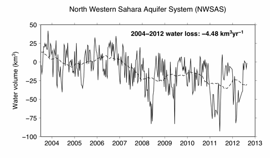
: Time series of regional 2° × 2° Gravity Recovery and Climate Experiment (GRACE) solutions of surface water mass change have been computed over Africa from 2003 to 2012 with a 10-day resolution by using a new regional approach. These regional maps are used to describe and quantify water mass change. The contribution of African hydrology to actual sea level rise is negative and small in magnitude (i.e., −0.1 mm/y of equivalent sea level (ESL)) mainly explained by the water retained in the Zambezi River basin. Analysis of the regional water mass maps is used to distinguish different zones of important water mass variations, with the exception of the dominant seasonal cycle of the African monsoon in the Sahel and Central Africa. The analysis of the regional solutions reveals the accumulation in the Okavango swamp and South Niger. It confirms the continuous depletion of water in the North Sahara aquifer at the rate of −2.3 km3/y, with a decrease in early 2008. Synergistic use of altimetry-based lake water volume with total water storage (TWS) from GRACE permits a continuous monitoring of sub-surface water storage for large lake drainage areas. These different applications demonstrate the potential of the GRACE mission for the management of water resources at the regional scale.
1. Introduction
Satellite gravimetry remains the only technique that provides information on the total water storage change at continental scales and gives access to groundwater variations when a priori information on surface and sub-surface reservoirs is available [1–3]. Data of the Gravity Recovery and Climate Experiment (GRACE) mission were widely used to estimate changes in land water storage and fluxes over Africa at basin to regional scales. By using the first two years (April 2002 to May 2003) of GRACE data, the study of [4] show that seasonal total water storage (TWS) variations vary between ±50 mm of TWS in the Congo and Niger basins. Time series of GRACE data allow us to estimate inter-annual variations and trends in TWS, as well as the contributions of TWS to sea level change for the largest drainage basins and lakes of Africa [5–12]. They were also used for comparisons, validation and calibration of hydrological model outputs at the basin scale and over large bio-climatic regions, such as the Sahel or West Africa [13–16]. Combined with external datasets in situ, GRACE data offer the unique opportunity to estimate groundwater storage variations for lake drainage areas [17,18] and large river basins [19] or at a regional scale [20], river discharges [21], evapotranspiration at the basin scale [22–24] and the water budget [25]. They were also used to determine the specific yield [26,27] and loading effects in the Sahel [28].
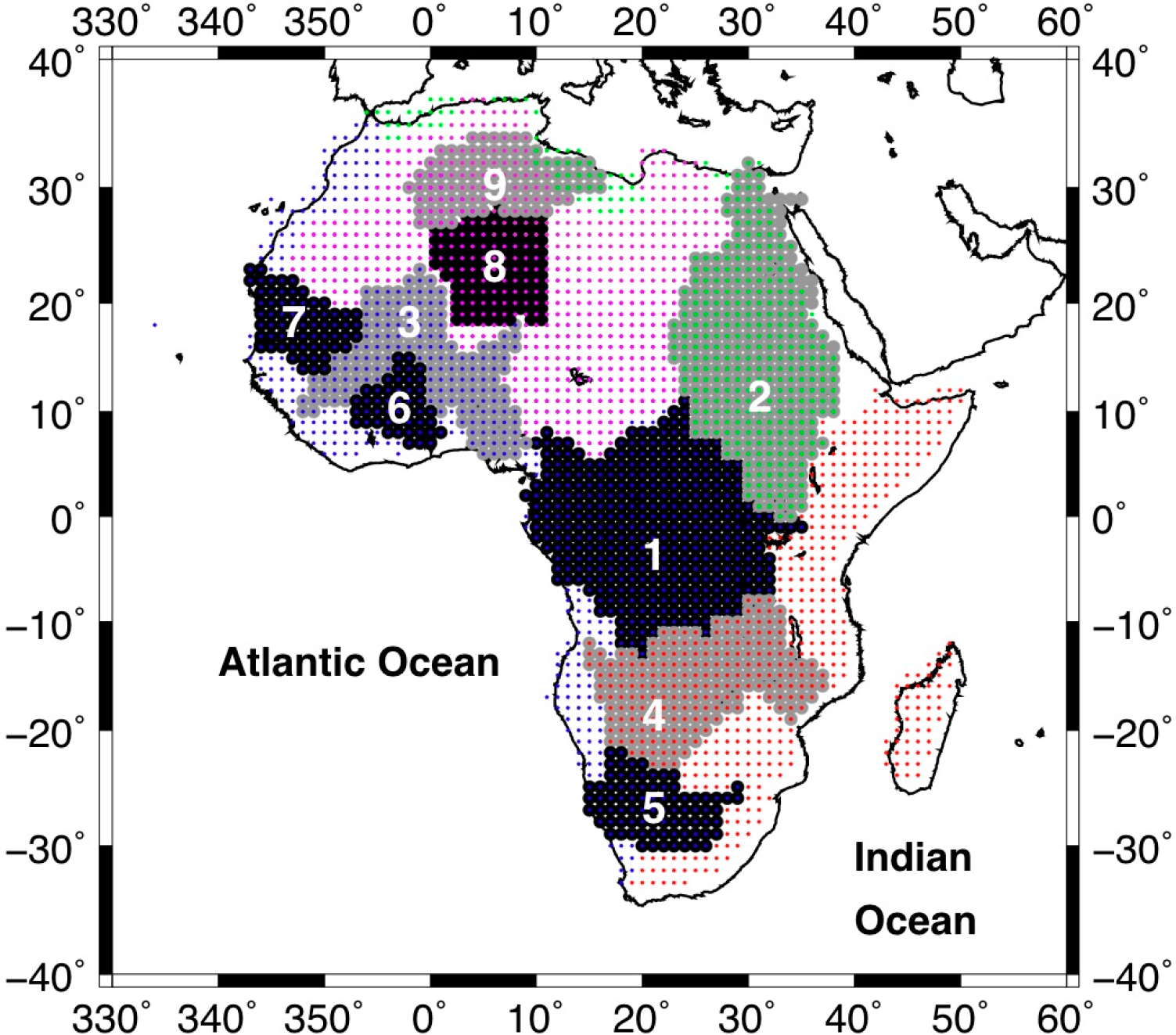
In the following section, the principle of classical satellite gravimetry and the particularities of the regional method for recovering water mass variations from GRACE satellite data are presented. Time series of 10-day 2° by 2° maps of water mass variations over Africa (30°W–60°E; 40°S–40°N) are computed from accurate K-band range rate (KBRR) residuals along daily GRACE orbits for the whole period of GRACE (2003–2012). Then, global solutions used for comparing our regional solutions computed over Africa are listed. The spatial averages of our African solutions over hydrological units (see the drainage basins and desert aquifer area in Figure 1) versus time are computed to establish water mass balances, and, thus, sea level contributions, for the recent period covered by the GRACE mission. For isolating the African regions that produce the largest contributions to the sea level mass balance (and the ones in water deficit), the first space and time modes of the variability of GRACE data are extracted using a principal component analysis (PCA). Then, the PCA modes are compared to pure seasonal, semi-seasonal and multi-year linear trend variations (e.g., African monsoon), so that multi-year water mass gains (or losses) can be located in Africa and quantified. Finally, combining water volumes derived from regional TWS solutions and radar altimetry measurements of the level of the lakes enables us to estimate the soil and groundwater variations over the East African Great Lakes.
2. Recovery of Surface Water Mass Changes by Space Gravimetry
Since its launch in 2002, the Gravity Recovery and Climate Experiment (GRACE) space mission has measured, for the first time, changes of total water storage (TWS), including surface water, soil, moisture and groundwater, with unprecedented centimeter accuracy in terms of geoid height. GRACE data have already demonstrated a strong potential for estimating hydrological system information, such as river discharges [29], evapotranspiration rate [22,30], groundwater variations [31–33] and the detection of extreme climate events, such as floods and droughts [34–40]. Several analysis centers, such as the Center for Space Research, University of Texas (CSR) in Austin (TX), the Jet Propulsion Laboratory (JPL) in Pasadena (CA), the GeoForschungsZentrum (GFZ) in Potsdam (Germany) and the Groupe de Recherche en Géodésie Spatiale (GRGS) in Toulouse (France), use Level 1-B GRACE observations to produce lists of monthly and 10-day global Stokes coefficients (i.e., spherical harmonics of the geopotential) up to harmonic degree 60 for CSR Release 5, 80 for GRGS RL03 and 90 for JPL and GFZ RL05; in other words, at the maximum surface resolution of 250–300 km. During the estimation process of the dimensionless Stokes coefficients from orbit data, the static gravity field and its time variations (i.e., atmospheric and ocean mass changes, including the effects of the periodic tides) are removed through a priori models describing these known gravitational accelerations. Therefore, the residuals correspond to the unmodeled contributions of mass to the observed gravity field and, mainly, the continental hydrology component.
Unfortunately, the correction models remain imperfect due to their lack of completeness in the description of water mass movements by omission and/or the lack of resolution, which represent important sources of error in the recovery of continental hydrology variations. As GRACE-based residual Stokes coefficients are averages over constant time intervals of 10 days or a month, errors in the correction models with periods from hours to days contaminate these GRACE solutions by aliasing and, thus, degrade their accuracy [41]. These effects of signal distortion deteriorate the quality of true water mass signals into other time frequencies and make these signals indistinguishable by sampling.
In the case of the GRACE orbit, hydrology-related signals are measured mainly along satellite tracks in the nearly latitudinal direction, but they are projected onto global spherical harmonics (SH) functions, which ensure the best spatial frequency representation. Because of this polar plane geometry of the GRACE orbit, this particular distribution of measurements creates north-south “stripes” in the 10-day and monthly GRACE solutions. Moreover, the determination of the SH coefficients leads to underdetermined systems of normal equations to be solved by creating correlations between SH coefficients of high degrees (i.e., >10–15) [42] and amplification of this orbit error and data noise [43].
Another problem while using SH is the “leakage” of energetic signals propagating over the entire sphere, as these global undulations come to pollute the water mass estimated in the region of interest. This is particularly the case of small regions that are not fully represented by the degree 60 truncated SH spectra of the GRACE solution (i.e., error by omission). Besides, different low-pass filtering techniques have been proposed, but they can partly cancel some of these effects [42,44,45]. The simplest way to increase the signal-to-noise ratio in estimation remains to average the signals over large surfaces of more than one million square kilometers, such as tropical drainage basins, to cancel the effects of the short wavelength SH undulations.
An alternative approach for estimating surface water mass densities in a region from GRACE data has been recently proposed by [46,47]. This new strategy is based on the optimal localization in space, instead of the best localization in spatial frequency, and leads theoretically to better spatial localization and resolution [48]. The authors of [47] have shown that this regional method offers a reduction of both north-south striping due to the distribution of GRACE satellite tracks and the temporal aliasing of correction models over South America [36] and Australia [49]. According to these two latter studies, regional maps present more realistic spatial and temporal patterns than the global solutions when compared to independent datasets of rainfall. The main modes of variability in South America coincide with the geographical limits of known hydrological units, such as individual groundwater layers [36]. In the present article, 10-day regional solutions over Africa are analyzed and compared to other datasets.
3. Methodology of the Regional Approach
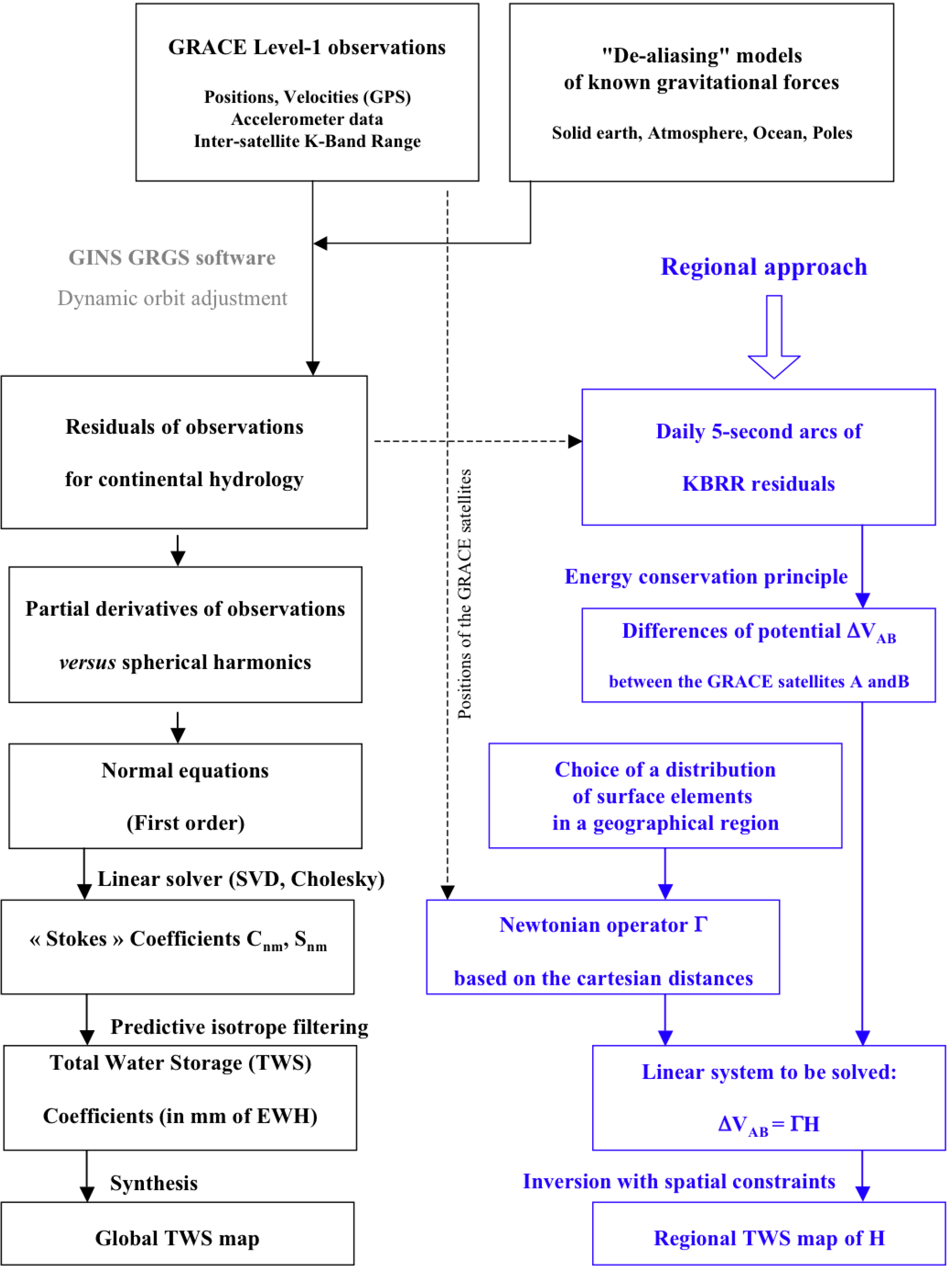
The two main steps of this regional method are: (1) using the principle of mechanical energy conservation to deduce the variations of difference potential anomalies (DPA) between the twin GRACE satellites, representing mainly the continental hydrology contribution, from the accurate along-track KBRR measurements; and (2) adjusting the equivalent water heights (EWH) of a network of juxtaposed 2° by 2° surface tiles by the linear inversion of the DPA passing over the considered region every 10 days [46,47]. This regional approach differs from the NASA “mascons” [50–52] as, instead of classical band-limited SH, the regional method imposes the geometry and the best spatial localization of surface hydrology structures by construction.
In the first step, KBRR observations are reduced by removing the contributions of known gravitational accelerations related to large-scale mass variations (i.e., atmosphere and ocean mass variations, polar movements, solid and oceanic tides, as well as the static gravity field of the Earth that represents 99% of the observed signals). This operation is made by iterative least squares adjustment of daily dynamical orbits using the Géodésie par Intégrations Numériques Simultanées (GINS) software [53,54]. Thanks to the measurements of on-board GRACE accelerometers, the effects of non-conservative forces are also removed from the KBRR observations in the orbit adjustment. KBRR residuals represent the cumulated contributions of unmodeled phenomena and, mainly, water storage change over continents. These residuals are related to the different accelerations of the two GRACE vehicles resulting from the gravity signals of continental hydrology, and they are easily converted into variations of kinetic energy differences. According to the principle of energy conservation, these kinetic energy difference variations directly correspond to potential energy differences, or in other words, DPA. To reduce unrealistic orbit errors at fractions of the satellite revolution periods and, thus, to avoid numerical instabilities in the following linear inversion, DPA arcs passing over Africa are linearly de-trended. It locally absorbs orbit error and keeps a subset of DPA short and medium wavelengths that are less than the latitudinal dimension of the considered region. The missing long-wavelength information of water mass change is from the first degrees of the GRGS solutions, and these large undulations are added to the DPA-derived regional solutions to complete the water mass signals after the inversion of residual DPA [36,47,49].
In the second step of the method, the Newtonian matrix A is defined from the positions of the two GRACE satellites and of the surface tiles, in a geocentric reference frame, according to Newton’s first law of attraction. This matrix relates each unknown EWH to the DPA observations inside the region during 10 successive days. As gravimetry inversion does not usually provide a unique solution, regularization strategies should be applied to find numerically-stable solutions, either based on the truncation of singular values [46] or by introducing an averaging radius [47].
This latter type of regularization consists of adding a spatial constraint matrix block C to the Newtonian matrix A. The coefficients of this extra matrix C are obtained by imposing each equivalent water height to be a linear combination of its neighbors weighted by the inverse of their angular distances and inside a maximum geographical radius r. In the case of spatial “averaging”, the coefficients for a given radius r should equal 1/P, as P is the number of surface tiles located at a distance lesser than r, and 0 elsewhere. Introduction of these linear constraints enables the ill-conditioned matrix A to be inverted. A good compromise for keeping enough hydrological details with no smoothing and limiting the increase of numerical noise was earlier found by considering a radius of r = 600 km over continental areas [47]. A simplified flowchart summarizing the estimation process of regional solutions is presented in the following Figure 2.
4. Datasets Used in This Study
4.1. 10-Day Regional GRACE Solutions for Africa
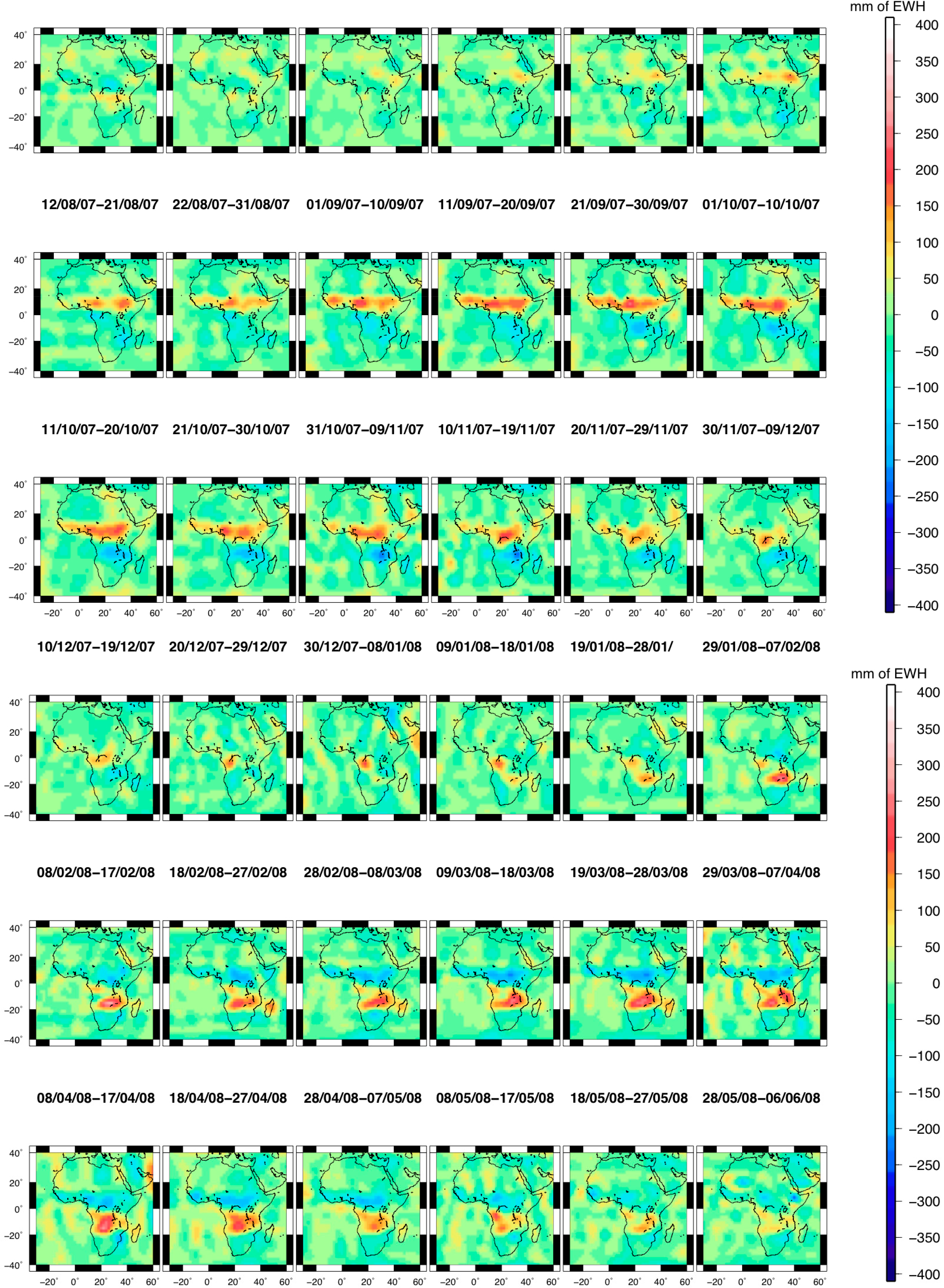
Daily arcs of five-second sampled K-band range (KBR) measurements of the inter-satellite velocity have been used in the GINS software [53,54] to adjust dynamical reference orbits. GRACE data are corrected from the known gravitational accelerations related to atmosphere and ocean mass redistributions, including tides and polar movements, using a priori global models. KBR rate residuals that represent mainly the continental hydrology have been converted into residual differences of potential (RDP), according to the conservation of the mechanical energy of the two GRACE vehicles versus time. Satellite tracks flying over Africa are selected, and each one is corrected from a least squares-adjusted linear trend. Following the two-step regional method explained in the previous section, time series of successive 10-day and 2° by 2° solutions of water mass change have been inverted over the whole African continent (30°W–60°E; 40°S–40°N) from RDP and, then, completed with the long wavelengths (>6700 km) of the GRGS GRACE solutions, or equivalently, the SH of degrees less than six, for the period 2003–2012. One complete year of regional solutions is displayed in Figure 3.
4.2. Global GRACE Solutions from Official Centers CSR, GFZ and JPL
Three processing centers, including the Center for Space Research (CSR), Austin, TX, USA, the GeoForschungsZentrum (GFZ), Potsdam, Germany, the Jet Propulsion Laboratory (JPL), Pasadena, CA, USA, and the Science Data Center (SDC) are in charge of the processing of the GRACE data and the production of Level-1 and Level-2 products. These products are distributed by the GFZ’s Integrated System Data Center (ISDC) [55] and the JPL’s Physical Oceanography Distributive Active Data Center (PODAAC) [56]. Preprocessing of Level-1 GRACE data (i.e., positions and velocities measured by GPS, accelerometer data and KBR inter-satellite measurements) is routinely made by the SDC, as well as monthly global GRACE gravity solutions (Level 2). These latter solutions consist of time series of monthly averages of Stokes coefficients (i.e., dimensionless spherical harmonics coefficients of geopotential) developed up to a degree between 50 and 120 that are adjusted from along-track GRACE measurements. A dynamical approach, based on the Newtonian formulation of the satellite’s equation of motion in an inertial reference frame, centered at the Earth’s center, combined with dedicated modeling of the gravitational and non-conservative forces acting on the spacecraft, is used to compute the monthly GRACE solutions [57]. During the estimation process, atmospheric and ocean barometric redistribution of mass variations are removed from the GRACE coefficients using European Centre for Medium-range Weather Forecasts (ECMWF) and National Centers for Environmental Prediction (NCEP) reanalysis for atmospheric mass variations and ocean tides, as well as global ocean circulation models. The GRACE coefficients are hence residuals that should represent mainly continental water storage, but also errors from the correction models and noise. The monthly GRACE solutions differ from one official provider from another due to the differences in the data processing, the choice of the correction models and the data selection for computing the monthly averages.
4.3. Global GRACE Solutions Provided by GRGS
These Level-2 European Improved Gravity model of Earth by New techniques solely from GRACE Satellite data (EIGEN) Release 04 10-day gravity models are derived from Level-1 GRACE measurements, including KBRR, from LAser GEOdynamics Satellites (LAGEOS) 1 and 2 Satellite Laser Ranging (SLR) data for the enhancement of lower harmonic degrees [47] and using an empirical stabilization approach without any post-processing smoothing or filtering. The 10-day Stokes coefficients are converted into terms of water mass coefficients from degree 2 up to degree 50–60 (i.e., spatial resolution of 400 km), expressed in EWH. Regular one-degree 10-day maps of surface water mass for the period 2002–2012 are derived from these latter SH water mass coefficients and made available for the last release (RL03) [58].
4.4. Independent Component Analysis of CSR, JPL and GFZ GRACE Solutions
Since the global GRACE solutions are unfortunately dominated by striping, our idea is to combine monthly solutions from different centers of analysis to extract the continental hydrology component from noisy sources by redundancy. A post-processing method based on independent component analysis (ICA) was applied to the Level-2 GRACE solutions from official providers (i.e., University of Texas–Center for Space Research (UTCSR), JPL and GFZ). Pre-filtered with 400-km radius Gaussian filters before applying an ICA, the Level-2 GRACE solutions need to be somehow low-passed filtered to not have a Gaussian distribution. When they are not filtered enough, they are still dominated by striping, and their distribution keeps being Gaussian. If they are too low-pass filtered, they correspond to the long wavelengths of the continental hydrology, and they also exhibit Gaussian properties. A compromise of ∼400 km to ensure no Gaussianity, and, thus, an efficient separation, has been proposed by [59] after several tests to extract most of the parts of the continental hydrology. Time series of ICA-based global maps of continental water mass changes computed over the period of March 2003–December 2010, are used for the comparison in this study [45]. For a given month, the ICA 400-km filtered solutions only differ by a scaling factor, so that only the GFZ-derived ICA 400-km filtered ones are presented.
4.5. Time Series of Altimetry-Derived Water Level of Lakes in East Africa
Satellite altimetry was originally designed to provide accurate measurements of the dynamic topography of the ocean [60]. Radar altimeters demonstrated strong capabilities to accurately estimate water levels over land and are now used for systematic monitoring of lakes [61,62], large rivers [63,64], wetlands and floodplains [65].
In this study, we used the time series of water levels derived from satellite altimetry measurements made available by the Hydroweb database at Laboratoire d’Etudes en Géophysique et Océanographie Spatiales (LEGOS)–Observatoire Midi-Pyrénées (OMP) [66] for four large lakes of East Africa (i.e., lakes Turkana, Victoria, Tanganyika and Malawi). All details about the processing of altimetry data and the computation of time series of water levels can be found in [61]. As these lakes do not have significant changes in area, the time series of water levels were simply converted into time series of water volumes using the mean surface of the lakes, as in [18]. The mean surfaces of the lakes are 8860, 68,800, 32,600 and 22,490 km2 for Turkana, Victoria, Tanganyika and Malawi lakes, respectively [67].
4.6. TRMM 3B43 Monthly Rainfall
In this study, we used the Tropical Rainfall Measuring Mission (TRMM) 3B43 product which is a combination of monthly rainfall at a spatial resolution of 0.25° from January 1998 to December 2012, and other data sources. This dataset is obtained by combining satellite information from the passive microwave imager (TMI) and precipitation radar (PR) onboard the Tropical Rainfall Measuring Mission (TRMM), a Japan-U.S. satellite launched in November 1997, the Visible and Infrared Scanner (VIRS) onboard the Special Sensor Microwave Imager (SSM/I) and rain gauge observations. The dataset results from the merging of the TRMM 3B42-adjusted merged infrared precipitation with the monthly accumulated Climate Assessment Monitoring System or Global Precipitation Climatology Center Rain Gauge analyses [68,69].
5. Results and Discussion
5.1. Residual Errors Estimated in the Arid Sahara Region
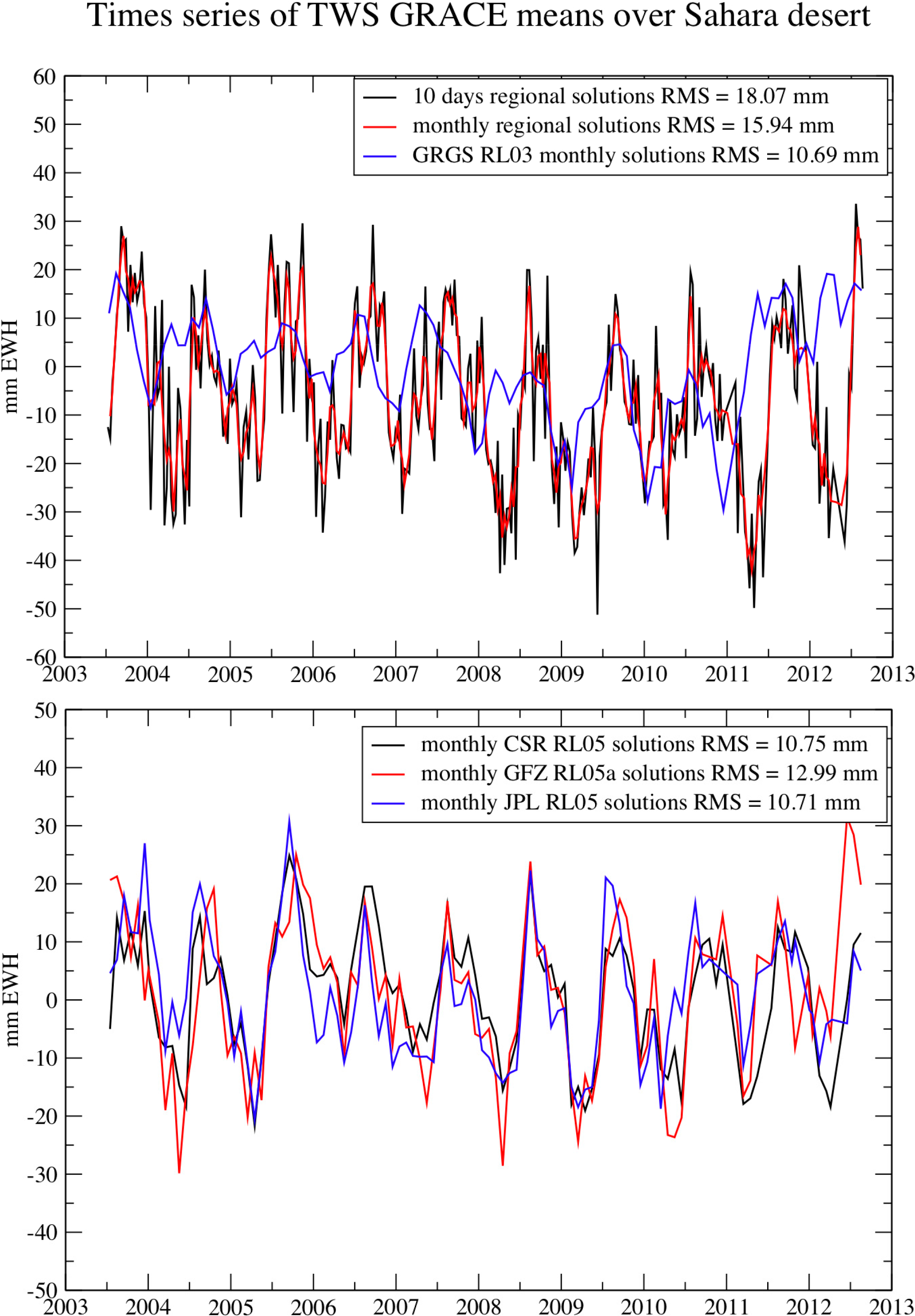
Figure 4 presents a time series of TWS in a desert area in the south of Algeria. As no hydrological variations are expected in such a very dry region, the residual water mass signals can be interpreted as a good indicator of the error in estimating water mass variations from GRACE orbit data. These recovery errors do not exceed 15–19 mm EWH RMS when GRACE solutions are averaged over a surface of ∼1 million square kilometers, consistently found by [70] from one year of global solutions. They also exhibit a seasonal cycle, in particular for the global and regional solutions (see Figure 4), which may result from leakage effects from surrounding areas polluting stronger water mass signals from the neighboring drainage basins, as well as errors from the a priori models used for correcting GRACE data and isolating the continental hydrology variations. For the global solutions, this latter effect is due to the spectral SH truncation of the global solutions at degree n = 60–90 (and of the underlying correcting models developed in SH for our regional solutions); in other words, the lack of spatial resolution to describe small objects, which creates unrealistic undulations propagating over the entire terrestrial sphere (i.e., leakage), as explained in Section 2.
5.2. Pre-Analysis of the 10-Day Maps of Water Mass over Africa
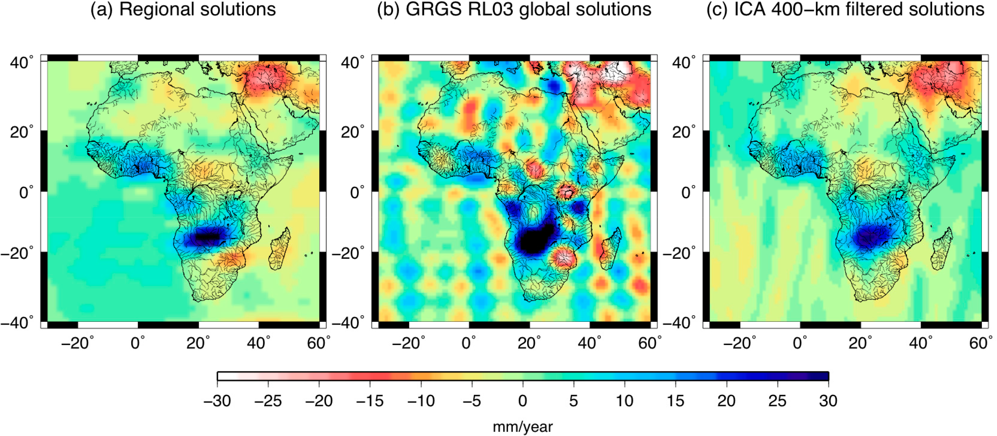
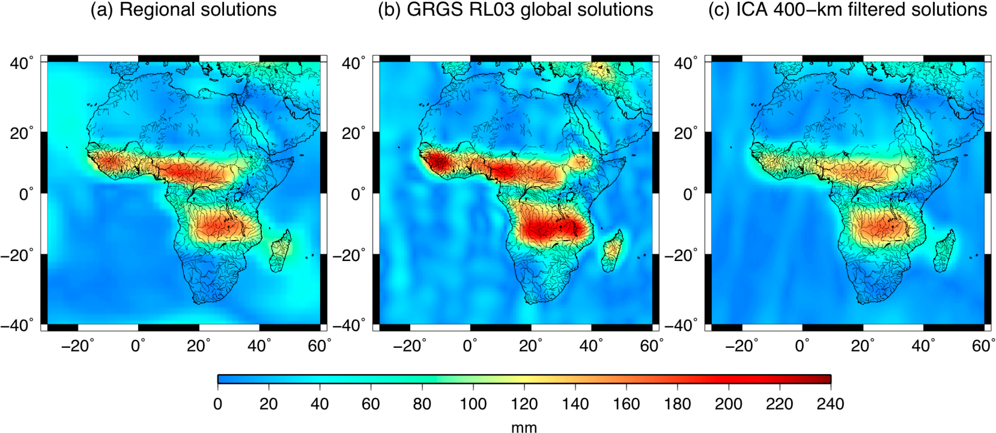
Annual, semi-annual amplitudes and linear trends for each surface element have been least squares adjusted from the complete series of 10-day regional solutions over the period 2003–2012. Dominant seasonal amplitudes of ±200 mm EWH are well located in the Sahel latitudinal band (i.e., 5°N–15°N), as expected, and in the Congo Basin (Figure 5).
The seasonal signature of the West African monsoon can also be seen [14]. It is slightly greater for the global GRGS and 400-km ICA solutions. Besides, negative linear trends are found in the Tigris-Euphrates region of −25 mm EWH per year, consistent with the recent depletion of water mass shown by previous studies [71]; there are important gains of water mass over the Okavango swamps, reaching more than +30 mm EWH per year (Figure 6). In the Niger basin, the gain remains close to +15 mm EWH per year. There are also slight depletions in the south of Lake Chad and in the south of Mozambique. Unrealistic north-south striping in the trend estimates is more important for the global GRGS solutions than for 400-km ICA solutions, as the combination of different global solutions by ICA reinforces the hydrological signals versus the noise. Striping does not appear in the linear trend map related to the regional solutions at all (e.g., see the residuals over the oceans).
5.3. Principal Component Analysis of the GRACE Datasets
Principal component analysis (PCA), or discrete Karhunen–Loève transform, consists of decomposing the time series of water mass maps (i.e., maps of regional water mass over Africa) into main space and time “modes” that are projections onto orthogonal directions (or the principal axis) of variability [72] (e.g., see [73] for the computational aspects). Before PCA decomposition, the time series of the regional solutions has been corrected from the dominant seasonal oscillation related to each surface element (see Figure 5) using 13-month window averaging.
5.3.1. First Mode of Variability: The Long-Term Behavior
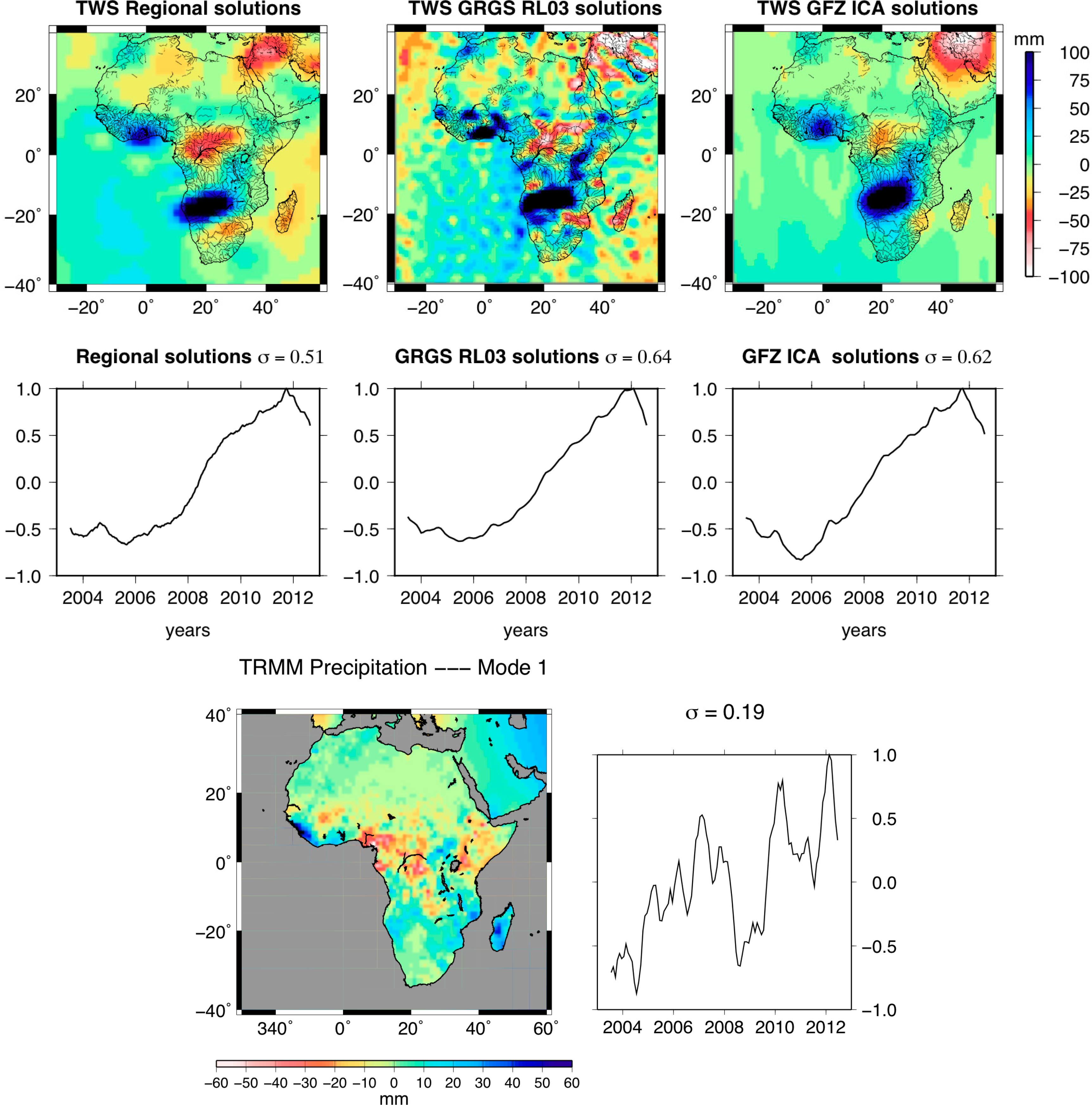
This mode corresponds to multi-year variations of water mass, since its temporal mode is characterized by a regular increase from 2006 to 2010 (Figure 7). All of the spatial modes range in ±100 mm EWH. This represents 50%–70% of the explained variance of the regional and smooth ICA solutions and 71% of the GRGS solutions.
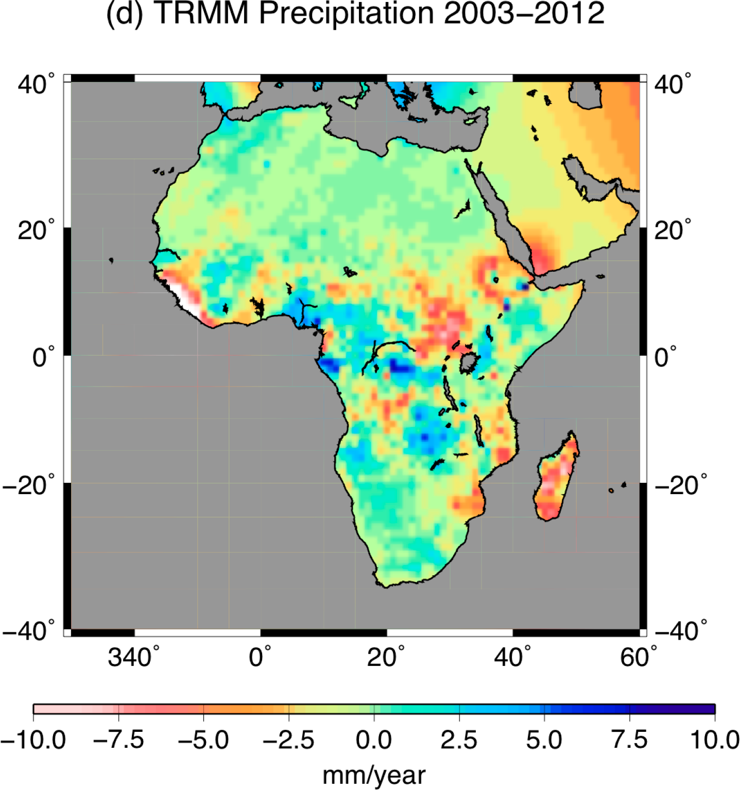
Thus, the corresponding spatial modes and the linear trend map presented in Figure 6 show similar patterns. The spatial mode associated with the monthly GRGS solutions contains unrealistic, short-scale undulations on the oceanic areas, as they are now derived from an empirical singular value decomposition (SVD) process of stabilization, and not a low-pass filtering, as for the GFZ, CSR and JPL solutions, which eliminates short wavelength more efficiently. The spatial components of the global solutions are affected by striping, especially the GRGS solutions, whereas no striping is visible in the regional water mass maps. There has been a dominant increase of mass in the Okavango swamp in the Zambezi River basin since 2006. The Okavango water system is an endorheic basin with no outlet to the sea, and it empties into the Kalahari Desert (∼18,000 square kilometers), known as the Okavango Delta. Water storage also increases regularly over Volta Lake in Ghana, which is the largest artificial lake in the world. An important mass loss is observed in the Congo basin, centered on the extensive floodplains known as the “Cuvette Centrale” (see [74] for their spatial extent), especially in the regional solutions. The signature of water mass depletion in the NWSAS region is also clearly visible in this first PCA mode associated with the regional solutions. The temporal component of the first mode of the TRMM rainfall also exhibits multi-annual variations (Figure 7). The corresponding spatial mode of the precipitation shows patterns that coincide with the modes of the PCA of regional/global GRACE solutions, in particular the long-term deficit of water for the Niger Delta and further over the land of Cameroon, as well as the increase along the coast of Guinea, Sierra Leone, Liberia, Ivory Coast and Ghana.
5.3.2. Second and Third Modes of Variability
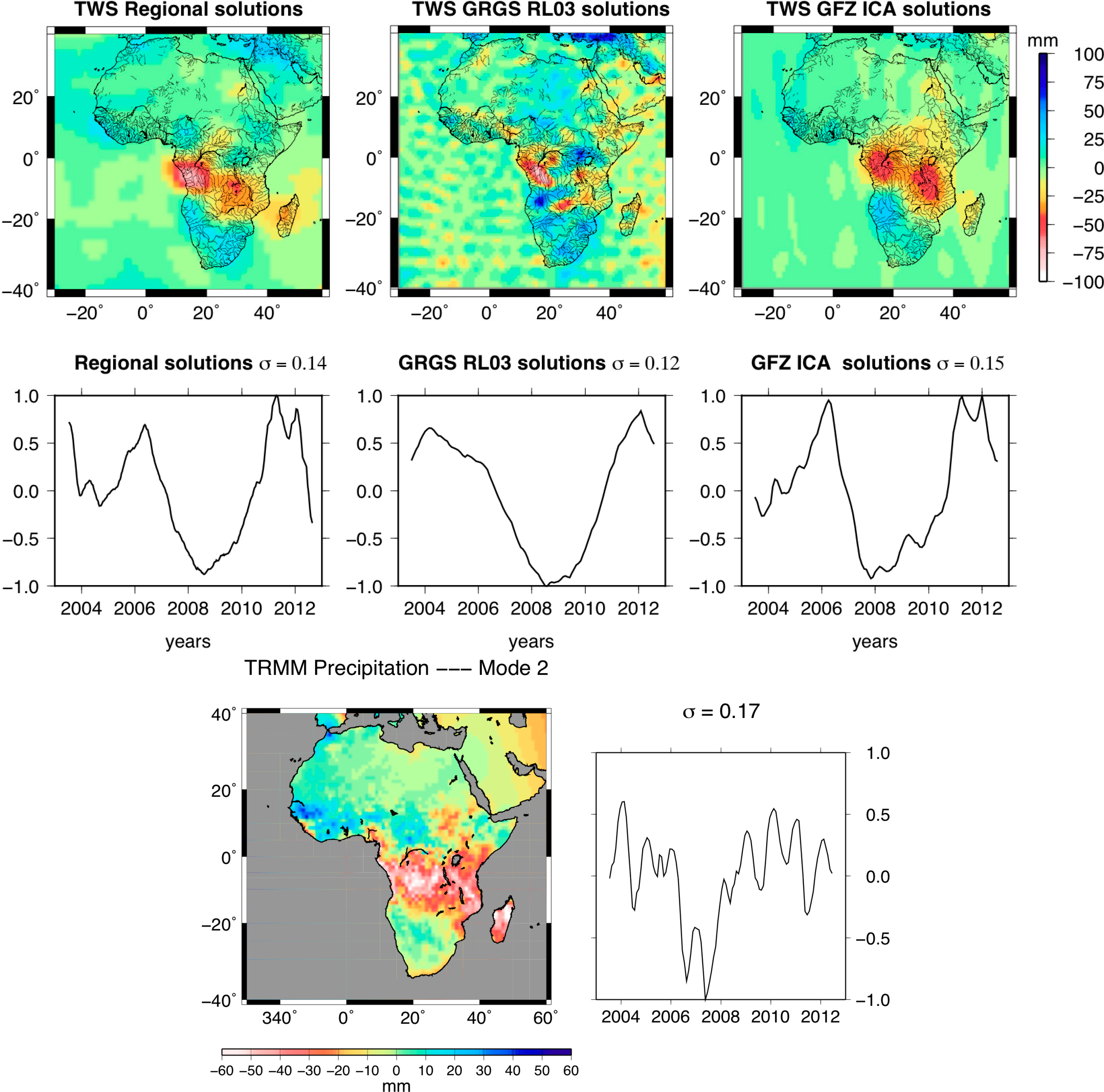
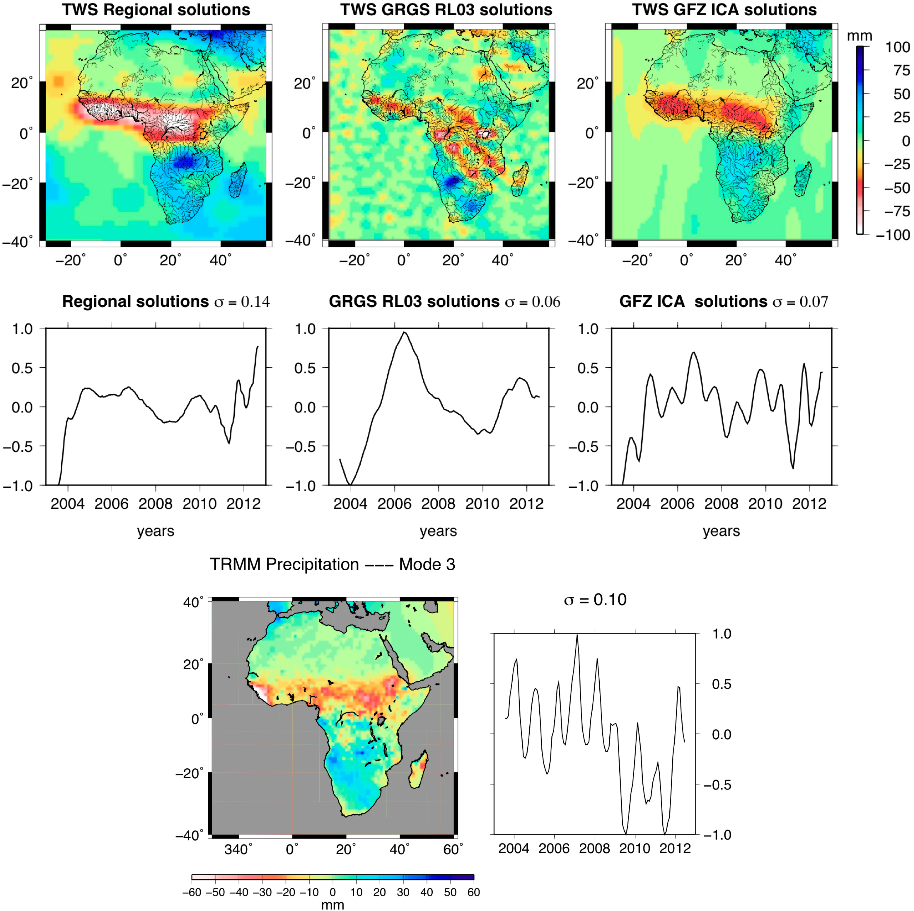
Second and third modes represent only 10%–15% and 6%–10% of the explained variances of the water mass signals, respectively (Figures 8 and 9). As the amplitudes of the third modes are smaller, it is more complicated to interpret its spatial and temporal patterns. The modes of global solutions still suffer from unrealistic striping that is visible over oceanic areas. In particular, the modes related to the GRGS solutions are affected by short wavelength noise. Except the JPL solutions, the temporal characteristics of the second PCA modes are two-year oscillations, as well as the maximum amplitudes of the spatial patterns on Central and Western Africa (i.e., northern part of the Congo River basin), including the Sahel, and along the Ivory Coast. As seasonal and semi-annual components have been removed before applying PCA, these patterns correspond to the bi-annual or quadrennial water mass variations related to the West African monsoon. Residual six-month and even multi-year oscillations appear for temporal modes of JPL.
As for the first mode of variability, similarities between PCA modes of GRACE and TRMM rainfall exist. The second PCA mode of the TRMM data is characterized by important amplitudes of precipitation in the southern tropics, in particular over the Congo Basin. This strong signal also appears in the second modes of GRACE datasets, but it is less visible in the case of GRGS solutions. The temporal mode of the rainfall data is shifted; it occurs ∼6 months sooner than the GRACE solutions (Figure 8). The third mode of rainfall is related to the African monsoon, as its main signature is located in the Sub-Saharan band, as for the spatial PCA modes of GRACE solutions (Figure 9).
5.4. Time Series of TWS Averaged over African River Drainage Basins
The masks used in this study come from the five-minute, 1/2° and 1° datasets of the continental watersheds and river networks for use in regional and global hydrologic and climate system modeling studies [75]. The 1° dataset is used for the drainage regions and the river watersheds, while the 0.5° dataset is used to define the drainage regions around the lakes. The coordinates of the drainage basin limits for each lake are obtained using the lake boundaries and the drainage network at 1/2°.
Time series of water mass for the main drainage basins of Africa over 2004–2012 (see Figure 1) have been computed as masked averages versus time and then converted into mm of equivalent sea level (ESL) profiles. In this latter operation, the water volume variations (i.e., equivalent water heights times the basin surface) are divided by the surface of the oceans (∼360 million square kilometers) and multiplied by −1. The per-basin time series of ESL are presented in Figure 10. Positive multi-year contributions to the sea level concern the Congo, Nile and Orange river basins, and they represent +0.044 mm/y in total, whereas the total negative contribution from the other basins is more important in magnitude (i.e., −0.123 mm/y), where the multi-year sea level contribution of the Zambezi Basin is the largest in magnitude (i.e., −0.1 mm/y). This region centered on the Okavango swamps and floodplains has been storing more and more water during the last decade.
As displayed in Figure 11, the sea level contributions averaged over large drainage areas to the Atlantic and Indian oceans and the Mediterranean Sea exhibit clear seasonal oscillations of amplitudes ±2, ±1 and ±0.5 mm of ESL, respectively. The seasonal contribution of land waters to the Indian Ocean (i.e., runoff along the southeastern coast of Africa) is in opposite phase with the two others. The sum of the contribution of these three large areas is negative (i.e., −0.088 mm per year); thus, the water mass balance of Africa for the period 2004–2012 indicates a gain of mass on the continent. In particular, the strongest multi-year trend magnitude is the one related to the Indian Ocean (i.e., −0.094 mm/y), as it shows a clear acceleration of the gain of water mass on land during recent years, passing from −0.034 mm/y before 2008 to −0.123 mm/y after 2008. A comparison with Figure 5 indicates that the latter contribution is driven by the long-term variations of the hydrology in the Zambezi River Basin. For the Atlantic and Mediterranean contributions, the positive ESL trends have been decreasing since 2008 from +0.138 mm/y and +0.030 mm/y down to +0.071 mm/y and +0.027 mm/y, respectively. Once the global isostatic adjustment (GIA) of the solid Earth from mainly post-glacial rebound and representing −0.3 mm/y is corrected [76,77], the net contribution of African rivers to sea level for 2004–2012 remains small, since it represents only ∼3% of the global increase of the sea level of 3.3 ± 0.4 mm/y measured by altimetry. This latter comparison suggests that the multi-year contribution of Africa hydrology remains in the total sea level error bar.
5.5. Detection of Recent Groundwater Withdraw of NWSAS Aquifer
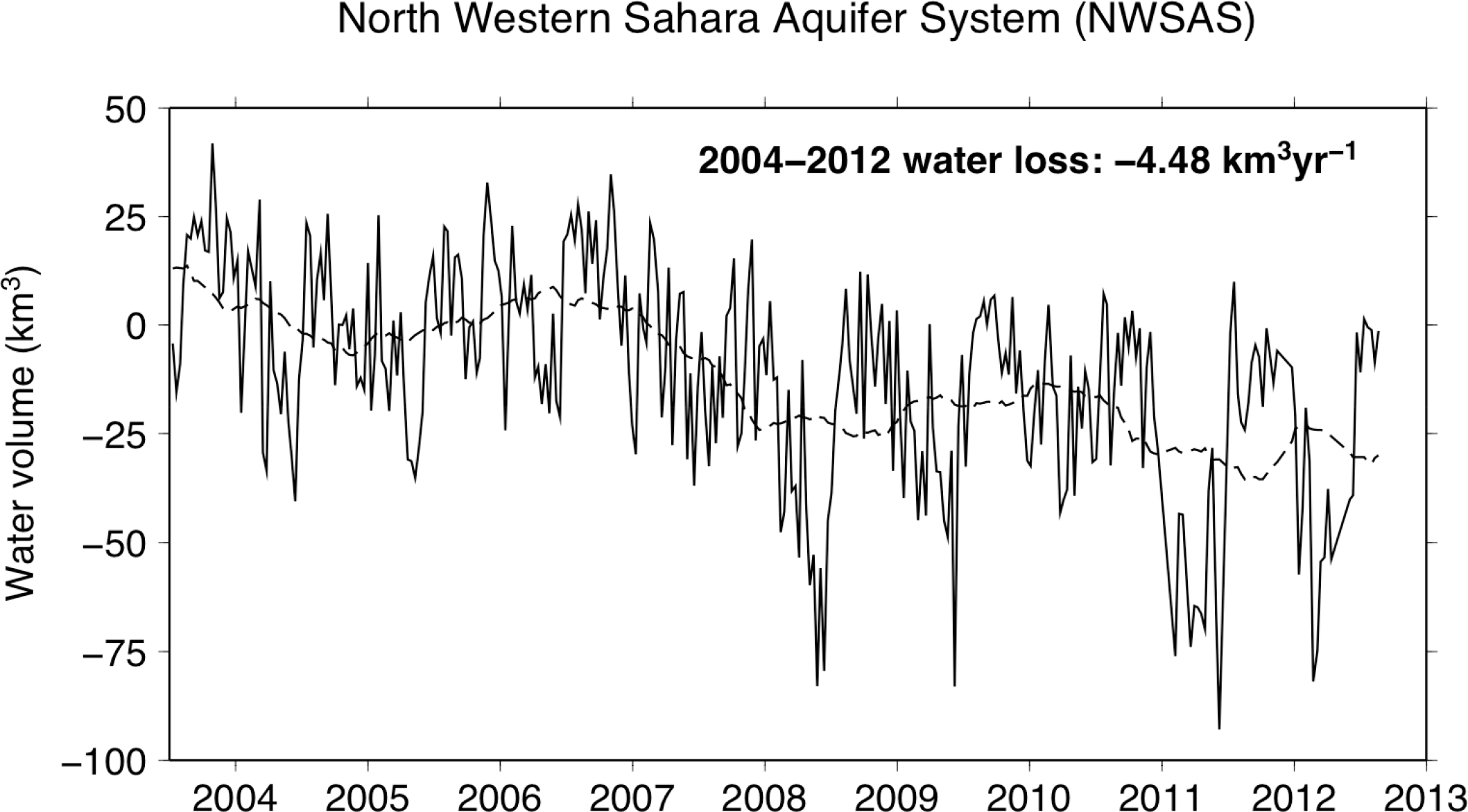
The NWSAS presented in Figure 1 (Area 9) is characterized by a transboundary “fossil” aquifer (i.e., with no meteoric water recharge) shared by three countries (i.e., 60% Algerian, 30% Libyan and 10% Tunisian surfaces) and in a critical situation of depletion by intense water pumping. While the groundwater imbalance is −2.2 km3 per year as estimated from historical records of piezometry before the year 2000 (see the report of [78]), our regional GRACE solutions averaged over the NWSAS indicate that the depletion of groundwater for the most recent decade is twice that, suggesting a worrying acceleration of the withdrawing of drinking water (Figure 12). In particular, a sudden loss of −25 km3 lasting a few months appears in the year 2007 between the periods January 2004–December 2007, and January 2008–January 2012. A comparison with the latter trends estimated considering the total GRACE period suggests that the rapid drop of groundwater in 2007–2008 remains exceptional (according to the dashed line). These are consistent with the recent estimates of groundwater loss from −2.2 km3/y in 2000 [78] to −2.75 km3/y in 2010 [79]. Time variations of TWS from GRACE appear reliable to directly and efficiently estimate the region-wide groundwater changes in a large aquifer system in arid areas and to provide useful information on groundwater recharge.
5.6. Subsurface Water Storage Changes by Combining Regional Solutions and Radar Altimeter Data
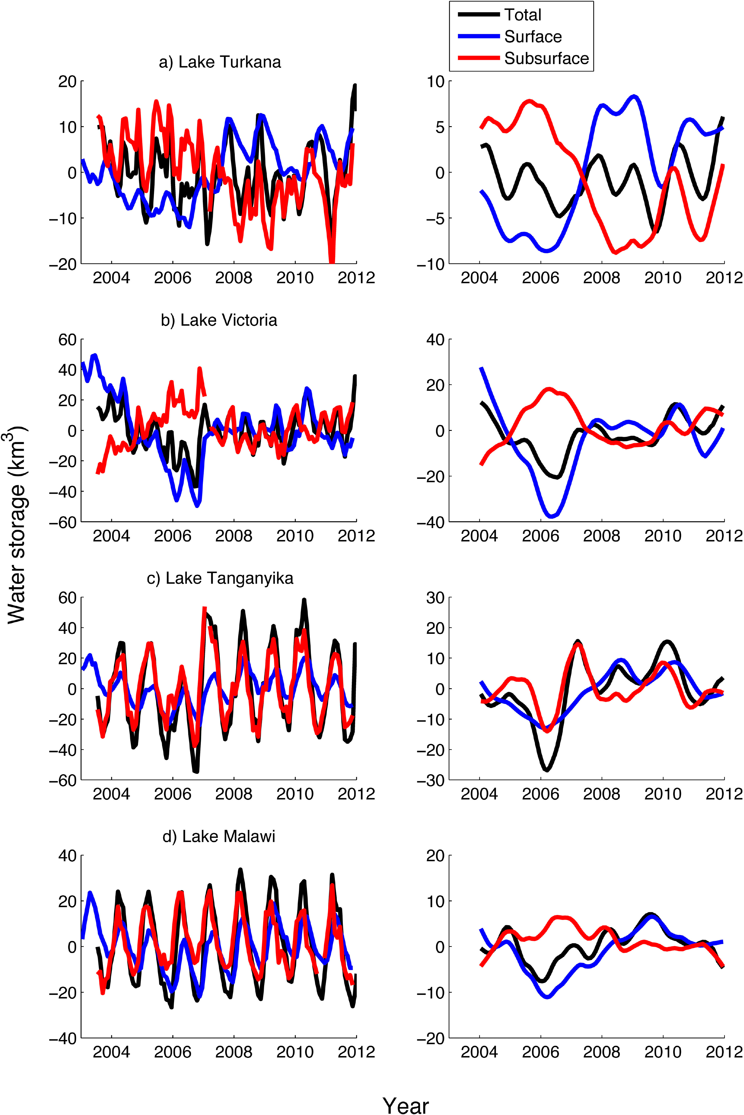
Time series of the subsurface waters (i.e., soil plus ground waters) were estimated by removing altimetry-based water levels of the main African lake, or reservoir waters, from the TWS measured by GRACE. As altimetry-based water levels from [78] have a temporal resolution of one month, the ten-day regional solutions were consequently averaged on monthly time periods before computing the mere difference. Anomalies of these residual subsurface waters, including groundwater, were estimated at a monthly time-scale as the difference between TWS and surface storage over the common period of availability of two datasets (i.e., mid-2003–2012). These anomalies are presented in Figure 13 for the largest East African lakes: Turkana, Victoria, Tanganyika and Malawi. They temporally and/or spatially extend the previous studies from [17,18,80], but using regional solutions instead of classical global ones.
Time variations of TWS and subsurface waters are well correlated for the three largest lakes, as the correlation coefficient R equals 0.75, 0.76 and 0.76 for Lake Victoria, Lake Tanganyika and Lake Malawi, but not for the smaller Lake Turkana, with R equal to 0.28. If the surface water storage represents only a small part of TWS variations, as for Lake Turkana over 2003–2013, its inter-annual variations are larger than the inter-annual TWS signals, similarly to what was found by [18]. The inter-annual signals of subsurface water presents three successive phases: from mid-2005 to mid-2008: they decreased at an average rate of −4 km3/y from mid-2008 to mid-2009 and remained stable; and since then, they present a bi-annual cycle of ±5 km3 of amplitude (Figure 13a). For Lake Victoria, the variations of the anomaly of water storage are greater for the surface reservoir than for the TWS. A larger decrease is observed for the anomaly of surface storage (−60 km3/y from 2004 to the beginning of 2006) than for TWS (−70 km3/y from 2004 to mid-2006) and the opposite up to the end of 2007, with increases of 40 and 20 km3/y for the surface water storage and TWS, respectively. Consequently, subsurface water is varying as the difference over the same time periods (Figure 13b). The results obtained with the regional solutions are very similar to those obtained by [18,81]. Nevertheless, [18] found larger variations of TWS than these from surface water, most likely because these authors included in the drainage areas of Lake Victoria the Kivu, Edouard, Albert and Kyoga lakes and their drainage areas, without adding their volume variations to the surface storage.
The TWS variations are dominated by the subsurface water component for Lake Tanganyika. A large variation of TWS, strongly impacting the subsurface water reservoir, is observed from 2005 to 2008, with a minimum reaching −40 km3 in the beginning of 2006 and a maximum of 30 km3 in the beginning of 2007. Smoother variations are present in the surface reservoir (Figure 13c).
As for Lake Victoria, TWS variations of Lake Malawi are dominated by the surface component, but the amplitudes of the surface reservoir are slightly greater than these from TWS at an inter-annual time scale. The time variations of the surface reservoir exhibit a steep decrease from 2004 to the beginning of 2006, followed by a significant increase up to mid-2009, whereas they are lower for TWS (Figure 13d).
These results demonstrate the strong capacities of multi-satellite observations to monitor quantitatively the changes in the storage of the surface and sub-surface reservoirs associated with climate variability and human activities at a regional scale. These remotely-sensed datasets are likely to have huge importance in regions where in situ data are sparse, while they have huge importance in terms of water supply for dense human populations. In the case of Lake Victoria, it directly supports 30 million people in terms of a freshwater supply [8] and indirectly another 340 million people along the Nile Basin [82], being the source of the White Nile.
6. Conclusions
In this paper, we present 10-day regional solutions of water mass change over Africa for the period 2003–2012, revealing the dominant seasonal and African monsoon signals (±250 mm EWH). Principal component analysis (PCA) of the GRACE datasets provided the main modes of variability of the surface water mass. Temporal and spatial patterns are consistent for the regional and global solutions. However, the regional solutions offer a better geographical localization of hydrological structures, while global solutions remain affected by aliasing errors (i.e., north-south striping). This is probably due to the benefit of details brought by GRACE short tracks into the regional solution, instead of considering band-limited spherical harmonics defined on the entire Earth.
Monitoring water supply by using these regional solutions enables us to confirm the long-term drought of the NWSAS aquifer and even to reveal the sudden water loss occurring in early 2008. In terms of large-scale mass balance, the small contribution of the African hydrology changes to global sea level rise for the period 2004–2012 remains negative, especially due to the gain of water mass in the swamp regions of the Zambezi River basin that represents −0.123 mm/y of ESL as a continuous deficit of the level for the Indian Ocean. Principal component analysis of the complete time series of regional GRACE solutions has been made to identify the separate contributions of the different African regions. In particular, the first mode of PCA, representing 50%–70% of the explained variance, reveals the long-term drought in East Africa and in the region of Lake Chad and, alternatively, the increase of water mass in the Okavango and Niger regions. The second PCA mode of 10% corresponds to an oscillation of two years over the Sahel and the central African regions. This latter mode is clearly related to the residuals of the dominant African monsoon. GRACE-derived TWS variations demonstrated strong capabilities for land water management in terms of monitoring the sub-surface changes alone over arid and semi-arid areas, such the NWAS basins, or in combination with altimetry-based water levels for lake drainage areas.
Acknowledgments
This work was supported by the CNES TOSCA grant “Surcharges et Propagation”. The authors would like to thank four anonymous reviewers for helping us in improving the quality of our manuscript.
Author Contributions
All three authors of the present work contributed to the writing of the manuscript, as well as the discussion of the results. The methodology for deriving regional solutions from accurate GRACE measurements had been previously developed by Guillaume Ramillien. Lucia Seoane computed the 10-day two-degree regional maps from daily GRACE orbits for the multi-year period, 2003–2012. Along-track residuals of gravity potential differences for continental hydrology were obtained using the GINS software developed by the GRGS group in Toulouse. In particular, Frédéric Frappart made the combination of the regional GRACE solutions with altimetry to derive the measured gravity contribution of sub-surface waters and to analyze their dynamics.
Conflicts of Interest
The authors declare no conflict of interest.
References
- Famiglietti, J.S.; Lo, M.; Ho, S.L.; Bethune, J.; Anderson, K.J.; Syed, T.H.; Swenson, S.C.; de Linage, C.R.; Rodell, M. Satellites measure recent rates of groundwater depletion in California’s Central Valley. Geophys. Res. Lett 2011. [Google Scholar] [CrossRef]
- Scanlon, B.R.; Faunt, C.C.; Longuevergne, L.; Reedy, R.C.; Alley, W.M.; McGuire, V.L.; MacMahon, P.B. Groundwater depletion and sustainability of irrigation in the US High Plains and Central Valley. Proc. Natl. Acad. Sci. USA 2012, 109, 9320–9325. [Google Scholar]
- Scanlon, B.R.; Longuevergne, L.; Long, D. Ground referencing GRACE satellite estimates of groundwater storage changes in the California Central Valley, USA. Water Resour. Res 2012. [Google Scholar] [CrossRef]
- Ramillien, G.; Frappart, F.; Cazenave, A.; Güntner, A. Time variations of land water storage from inversion of 2-years of GRACE geoids. Earth Planet. Sci. Lett 2005, 235, 283–301. [Google Scholar]
- Crowley, J.W.; Mitrovica, J.X.; Bailey, R.C.; Tamisiea, M.E.; Davis, J.L. Land water storage within the Congo basin inferred from GRACE satellite gravity data. Geophys. Res. Lett 2006. [Google Scholar] [CrossRef]
- Papa, F.; Güntner, A.; Frappart, F.; Prigent, C.; Rossow, W.B. Variations of surface water extent and water storage in large river basins: A comparison of different global data sources. Geophys. Res. Lett 2008. [Google Scholar] [CrossRef]
- Ramillien, G.; Bouhours, S.; Lombard, A.; Cazenave, A.; Flechtner, F.; Schmidt, R. Land water storage contribution to sea levelfrom GRACE geoid data over 2003–2006. Glob. Planet. Chang 2008, 60, 381–392. [Google Scholar]
- Lee, H.; Beighley, R.E.; Alsdorf, D.; Jung, H.; Shum, C.; Duan, J.; Guo, J.; Yamazaki, D.; Andreadis, K. Characterization of terrestrial water dynamics in the Congo Basin using GRACE and satellite radar altimetry. Remote Sens. Environ 2011, 115, 3530–3538. [Google Scholar]
- Awange, J.L.; Sharifi, M.A.; Ogonda, G.; Wickert, J.; Grafarend, E.W.; Omulo, M.A. The falling Lake Victoria water level: GRACE, TRIMM and CHAMP satellite analysis of the lake basin. Water Resour. Manag 2008, 22, 775–796. [Google Scholar]
- Awange, J.L.; Ong’ang’a, O. Lake Victoria: Ecology Resource and Environment; Springer: Berlin, Germany, 2006; p. 354. [Google Scholar]
- Deus, D.; Gloaguen, R.; Krause, P. Water balance modeling in a semi-arid environment with limited in situ data using remote sensing in Lake Manyara, East African Rift, Tanzania. Remote Sens 2013, 5, 1651–1680. [Google Scholar]
- Jensen, L.; Rietbrock, R.; Kusche, J. Land water contribution to sea level from GRACE and Jason-1 measurements. J. Geophys. Res.: Oceans 2013, 118, 212–226. [Google Scholar]
- Klees, R.E.; Zapreeva, A.; Winsemius, H.C.; Savenije, H.H.C. The bias in GRACE estimates of continental water storage variations. Hydrol. Earth Syst. Sci 2007, 11, 1227–1241. [Google Scholar]
- Grippa, M.; Kergoat, L.; Frappart, F.; Araud, Q.; Boone, A.; de Rosnay, P.; Lemoine, J.-M.; Gascoin, S.; Balsamo, G.; Ottlé, C.; et al. Land water storage over West Africa estimated by GRACE and land surface model. Water Resour. Res 2011. [Google Scholar] [CrossRef]
- Milzow, C.; Krogh, P.E.; Bauer-Gottwein, P. Combining satellite radar altimetry, SAR surface soil moisture and GRACE total storage changes for hydrological calibration in a large poorly gauged catchment. Hydrol. Earth Syst. Sci 2011, 15, 1729–1743. [Google Scholar]
- Xie, H.; Longuevergne, L.; Ringler, C.; Scanlon, B.R. Calibration and evaluation of a semi-distributed watershed model of a sub-saharan Africa using GRACE data. Hydrol. Earth Syst. Sci 2012, 16, 3083–3099. [Google Scholar]
- Swenson, S.; Wahr, J. Monitoring the water balance of Lake Victoria, East Africa, from space. J. Hydrol 2009. [Google Scholar] [CrossRef]
- Becker, M.; Llovel, W.; Cazenave, A.; Güntner, A.; Crétaux, J.-F. Recent hydrological behaviour of the East African Great Lakes region inferred from GRACE, satellite altimetry and rainfall observations. Comptes Rendus Géosci 2010. [Google Scholar] [CrossRef]
- Bonsor, H.C.; Mansour, M.M.; MacDonald, A.M.; Hughes, A.G.; Hipkin, R.G.; Bedada, T. Interpretation of GRACE data of the Nile Basin using a groundwater recharge model. Hydrol. Earth Syst. Sci 2010, 7, 4501–4533. [Google Scholar]
- Henry, C.M.; Allen, D.M.; Huang, J. Groundwater storage variability and annual recharge using well-hydrograph and GRACE satellite data. Hydrogeol. J. 2011, 19, 741–755. [Google Scholar]
- Syed, T.H.; Famiglietti, J.S.; Chambers, D.P. GRACE-based estimates of terrestrial freshwater discharge from basin to continental scales. Hydrogeol. J. 2009, 10, 22–40. [Google Scholar]
- Ramillien, G.; Frappart, F.; Güntner, A.; Ngo-Duc, T.; Cazenave, A.; Laval, K. Time variations of regional evapotranspiration rate from Gravity Recovery and Climate Experiment (GRACE) satellite gravimetry. Water Resour. Res 2006. [Google Scholar] [CrossRef]
- Rodell, M.; McWilliams, E.B.; Famiglietti, J.S.; Beaudoing, H.K.; Nigro, J. Estimating evapotranspiration using an observation based terrestrial water budget. Hydrol. Process 2011, 25, 4083–4092. [Google Scholar]
- Long, D.; Longuevergne, L; Scanlon, B.R. Uncertainty in evapotranspiration from land surface modeling, remote sensing, and GRACE satellites. Water Resour. Res 2014, 50, 1131–1151. [Google Scholar]
- Trenberth, K.E.; Fasullo, J.T. Regional energy and water cycles: Transports from ocean to land. J. Clim 2013, 26, 7837–7851. [Google Scholar]
- Pfeffer, J.; Boucher, M.; Hinderer, J.; Favreau, G.; Boy, J.-P.; de Linage, C.; Cappelaere, B.; Luck, B.; Oi, M.; le Moigne, M. Local and global hydrological contribution to time variable gravity in southwest Niger. Geophys. J. Int 2011, 184, 661–672. [Google Scholar]
- Hector, B.; Seguis, L.; Hinderer, J.; Descloitres, M.; Vouillamoz, J.-M.; Wubda, M.; Boy, J.-P.; Luck, B.; le Moigne, N. Gravity effect of water storage changes in a weathered hard-rock aquifer in West Africa: Results from joint absolute gravity, hydrological monitoring and geophysical prospection. Geophys. J. Int 2013, 194, 737–750. [Google Scholar]
- Nahmani, S.; Bock, O.; Bouin, M.-N.; Santamaría-Gómez, A.; Boy, J.-P.; Collilieux, X.; Métivier, L.; Panet, I.; Genthon, G.; de Linage, C.; et al. Hydrological deformation induced by the West African Monsoon: Comparison of GPS, GRACE and loading models. J. Geophys. Res.: Solid Earth 2012. [Google Scholar] [CrossRef]
- Syed, T.H.; Famiglietti, J.S.; Rodell, M.; Chen, J.; Wilson, C.R. Analysis of terrestrial water storage changes from GRACE and GLDAS. Water Resour. Res 2008. [Google Scholar] [CrossRef]
- Rodell, M.; Famiglietti, J.S.; Chen, J.; Seneviratne, S.I.; Viterbo, P.; Holl, S.; Wilson, C.R. Basin sacle estimate of evapotranspiration using GRACE and other observations. Geophys. Res. Lett 2004. [Google Scholar] [CrossRef]
- Rodell, M.; Chen, J.; Kato, H.; Famiglietti, J.S.; Nigro, J.; Wilson, C.R. Estimating grounwater storage changes in the Mississippi River basin (USA) using GRACE. Hydrogeol. J. 2007, 15, 159–166. [Google Scholar]
- Leblanc, M.; Tregoning, P.; Ramillien, G.; Tweed, S.; Fakes, A. Basin scale, integrated observations of the early 21st century multi-year drought in Southeast Australia. Water Resour. Res 2009. [Google Scholar] [CrossRef]
- Taylor, R.G.; Scanlon, B.R.; Döll, P.; Rodell, M.; van Beek, R.; Wada, Y.; Longuevergne, L.; Leblanc, M.; Famiglietti, J.S.; Edmunds, M.; et al. Ground water and climate change. Nat. Clim. Chang 2013. doi: 10/1038/nclimate1744. [Google Scholar]
- Andersen, O.B.; Seneviratne, S.I.; Hinderer, J.; Viterbo, P. GRACE-derived terrestrial water storage depletion associated with the 2003 European heat wave. Geophys. Res. Lett 2005. [Google Scholar] [CrossRef]
- Frappart, F.; Papa, F.; Santos da Silva, J.; Ramillien, G.; Prigent, C.; Seyler, F.; Calmant, S. Surface freshwater storage and dynamics in the Amazon basin during the 2005 exceptional drought. Environ. Res. Lett 2012. [Google Scholar] [CrossRef]
- Frappart, F.; Seoane, L.; Ramillien, G. Validation of GRACE-derived water mass storage using a regional approach over South America. Remote Sens. Environ 2013, 137, 69–83. [Google Scholar]
- Houborg, R.; Rodell, M.; Li, B.; Reichle, R.; Zaitchik, B.F. Drought indicators based on model-assimilated Gravity Recovery and Climate Experiment (GRACE) terrestrial water storage observations. Water Resour. Res 2012. [Google Scholar] [CrossRef]
- Chen, J.L.; Wilson, C.R.; Tapley, B.D. The 2009 exceptional Amazon flood and interannual terrestrial water storage change observed by GRACE. Water Resour. Res 2010. [Google Scholar] [CrossRef]
- Chen, J.L.; Wilson, C.R.; Tapley, B.D.; Longuevergne, L.; Yang, Z.L.; Scanlon, B.R. Recent La Plata basin drought conditions observed by satellite gravimetry. J. Geophys. Res.: Atmos 2010. [Google Scholar] [CrossRef]
- Long, D.; Scanlon, B.R.; Longuevergne, L; Sun, A.; Fernando, N.; Save, H. GRACE satellite monitoring of large depletion in water storage in response to the 2011 drought in Texas. Geophys. Res. Lett 2013, 40, 3395–3401. [Google Scholar]
- Duan, J.; Shum, C.K.; Guo, J.; Huang, Z. Uncovered spurious jumps in the GRACE atmospheric de-aliasing data: Potential contamination of GRACE observed mass change. Geophys. J. Int 2012, 191, 83–87. [Google Scholar]
- Swenson, S.C.; Wahr, J. Post-processing removal of correlated errors in GRACE data. Geophys. J. Int 2006. [Google Scholar] [CrossRef]
- Himanshu, S.; Bettadpur, S.; Tapley, B.D. Reducing errors in the GRACE gravity solutions using regularization. J. Geodesy 2012, 86, 695–711. [Google Scholar]
- Klees, R.; Revtova, E.A.; Gunter, B.C.; Ditmar, P.; Oudman, E.; Winsemius, H.C.; Savenije, H.H.G. The design of an optimal filter for monthly GRACE gravity models. Geophys. J. Int 2008, 175, 417–432. [Google Scholar]
- Frappart, F.; Ramillien, G.; Leblanc, M.; Tweed, S.O.; Bonnet, M.-P.; Maisongrande, P. An independent component analysis approach for filtering continental hydrology in the GRACE gravity data. Remote Sens. Environ 2011, 115, 187–204. [Google Scholar]
- Ramillien, G.; Biancale, R.; Gratton, S.; Vasseur, X.; Bourgogne, S. GRACE-derived surface mass anomalies by energy integral approach. Application to continental hydrology. J. Geodesy 2011, 85, 313–328. [Google Scholar]
- Ramillien, G.; Seoane, L.; Frappart, F.; Biancale, R.; Gratton, S.; Vasseur, X.; Bourgogne, S. Constrained regional recovery of continental water mass time-variations from GRACE based geopotential anomalies over South America. Surv. Geophys 2012, 33, 887–905. [Google Scholar]
- Freeden, W.; Schreiner, M. Spherical Functions of Mathematical Geosciences: A Scalar, Vectorial and Tensorial Setup; Springer: Berlin, Germany, 2008. [Google Scholar]
- Seoane, L.; Ramillien, G.; Frappart, F.; Leblanc, M. Regional GRACE-based estimates of water mass variations over Australia: Validation and interpretation. Hydrol. Earth Syst. Sci 2013, 17, 4925–4939. [Google Scholar]
- Rowlands, D.D.; Ray, R.D.; Chinn, D.S.; Lemoine, F.G. Short-arc analysis of intersatellite tracking data in a gravity mapping mission. J. Geodesy 2002. [Google Scholar] [CrossRef]
- Rowlands, D.D.; Luthcke, S.B.; Klosko, S.M.; Lemoine, F.G.; Chinn, D.S.; McCarthy, J.J.; Cox, C.M.; Anderson, O.B. Resolving mass flux at high spatial and temporal resolution using GRACE intersatellite measurements. Geophys. Res. Lett 2005. [Google Scholar] [CrossRef]
- Lemoine, F.G.; Luthcke, S.B.; Rowlands, D.D.; Chinn, D.S.; Klosko, S.M.; Cox, C.M. The use of mascons to resolve time-variable gravity from GRACE. In Dynamic Planet; Springer: Berlin, Germany, 2007; pp. 231–236. [Google Scholar]
- Lemoine, J.-M.; Bruinsma, S.; Loyer, S.; Biancale, R.; Marty, J.-C.; Pérosanz, F.; Balmino, G. Temporal gravity field models inferred from GRACE data. Adv. Space Res 2007, 39, 1620–1629. [Google Scholar]
- Bruinsma, S.; Lemoine, J.-M.; Biancale, R.; Valès, N. CNES/GRGS 10-day gravity models (release 2) and their evaluation. Adv. Space Res 2010, 45, 587–601. [Google Scholar]
- GFZ Potsdam Information Systems & Data Center. Available online: http://isdc.gfz-potsdam.de (accessed on 22 July 2014).
- Physical Oceanography Distributed Active Archive Data. Available online: http://podaac-www.jpl.nasa.gov (accessed on 31 July 2014).
- Schmidt, R.; Flechtner, F.; Meyer, U.; Neumayer, K.-H.; Dahle, Ch.; Koenig, R.; Kusche, J. Hydrological signals observed by GRACE satellites. Surv. Geophys 2008, 29, 319–334. [Google Scholar]
- Groupe de Recherche en Géodésie Spatiale. Available online: http://grgs.obs-mip.fr (accessed on 22 July 2014).
- Frappart, F.; Ramillien, G.; Maisongrande, P.; Bonnet, M.-P. Denoising satellite gravity signals by independent component analysis. IEEE Geosci. Remote Sens. Lett 2010, 7, 421–425. [Google Scholar]
- Fu, L.L.; Cazenave, A. Satellite Altimetry and Earth Sciences, A Handbook of Techniques and Applications, International Geophysics Series; Academic Press: San Diego, FL, USA, 2001; Volume 69. [Google Scholar]
- Crétaux, J.-F.; Jelinski, W.; Calmant, S.; Kouraev, A.; Vuglinski, V.; Bergé-Nguyen, M.; Gennero, M.-C.; Niño, F.; Abarca del Rio, R.; Cazenave, A.; et al. SOLS: A lake database to monitor in near real time water level and storage variations from remote sensing data. J. Adv. Space Res 2011. [Google Scholar] [CrossRef]
- Ričko, M.; Birkett, C.M.; Carton, J.A.; Crétaux, J.-F. Intercomparison and validation of continental water level products derived from satellite radar altimetry. J. Appl. Remote Sens 2012. [Google Scholar] [CrossRef]
- Frappart, F.; Calmant, S.; Cauhopé, M.; Seyler, F.; Cazenave, A. Preliminary results of ENVISAT RA-2 derived water levels validation over the Amazon basin. Remote Sens. Environ 2006, 100, 252–264. [Google Scholar]
- Santos da Silva, J.; Calmant, S.; Seyler, F.; Rottuno Filho, O.C.; Cochonneau, G.; Mansur, W.J. Water levels in the Amazon basin derived from the ERS-2 and ENVISAT radar altimetry missions. Remote Sens. Environ 2010, 114, 2160–2181. [Google Scholar]
- Frappart, F.; Seyler, F.; Martinez, J.-M.; Leon, J.G.; Cazenave, A. Floodplain water storage in the Negro River basin estimated from microwave remote sensing of inundation area and water levels. Remote Sens. Environ 2005, 99, 387–399. [Google Scholar]
- Hydrology from Space. Lakes, Rivers and Wetlands Water Levels from Satellite Altimetry. Available online: http://www.legos.obs-mip.fr/soa/hydrologie/hydroweb/ (accessed on 22 July 2014).
- Spigel, R.H.; Coulter, G.W. Comparison of hydrology and physical limnology of the East African Great lakes: Tanganyika, Malawi, Victoria, Kivu and Turkana (with references to some North American Great lakes). In The Limnology, Climatology and Paleoclimatology of the East African Lakes; Johnson, T.C., Odada, E.O., Eds.; Gordon & Breach Publishers: Amsterdam, The Netherlands, 1996; pp. 103–135. [Google Scholar]
- Huffmann, G.J.; Adler, R.F.; Rudolf, B.; Schneider, U; Keehn, P.R. Global precipitation estimates based on a technique for combining satellite-based estimates, rain gauge analysis, and NWP model precipitation information. J. Clim 1995, 8, 1284–1295. [Google Scholar]
- Huffmann, G.J.; Adler, R.F.; Bolvin, D.T.; Gu, G.; Nelkin, E.J.; Bowman, K.P.; Hong, Y.; Stocker, E.F.; Wolf, D.B. The TRMM Multi-satellite Precipitation Analysis (TMPA): Quasi-global, multi-year, combined-sensor precipitation estimates at fine scale. J. Hydrometeorol 2007, 8, 38–55. [Google Scholar]
- Seo, K.-W.; Wilson, C.R.; Famiglietti, J.S.; Chen, J.L.; Rodell, M. Terrestrial water mass load changes from Gravity Recovery and Climate Experiment (GRACE). Water Resour. Res 2006. [Google Scholar] [CrossRef]
- Voss, K.A.; Famiglietti, J.S.; Lo, M.; de Linage, C.; Rodell, M.; Swenson, S.C. Groundwater depletion in the Middle East from GRACE with implications for transboundary water management in the Tigris-Euphrates-Western Iran region. Water Resour. Res 2013, 49, 904–914. [Google Scholar]
- Preisendorfer, R. Principal Component Analysis in Meteorology and Oceanography; Elsevier: Amsterdam, The Netherlands, 1988. [Google Scholar]
- Toumazou, V.; Crétaux, J.F. Using a Lanczos eigensolver in the computation of empirical orthogonal functions. Mon. Month Rev 2001, 129, 1243–1250. [Google Scholar]
- Betbeder, J.; Gond, V.; Frappart, F.; Baghdadi, N.; Briant, G.; Bartholomé, E. Mapping of Central Africa forested wetlands using remote sensing. IEEE J. Sel. Top. Earth Observ. Remote Sens 2014, 7, 531–542. [Google Scholar]
- Graham, S.T.; Famiglietti, J.S.; Maidment, D.R. 5-minute, 1/2° and 1° data sets of continental watersheds and river networks for use in regional and global hydrologic and climate system modeling studies. Water Resour. Res 1999, 35, 583–587. [Google Scholar]
- Cazenave, A.; Dominh, K.; Guinehut, S.; Berthier, E.; Llovel, W.; Ramillien, G.; Ablain, M; Larnicol, G. Sea level budget over 2003–2008: A reevaluation from GRACE space gravimetry, satellite altimetry and Argo. Glob. Planet. Chang 2009, 65, 83–88. [Google Scholar]
- Cazenave, A.; Llovel, W. Contemporary sea level rise. Annu. Rev. Mar. Sci 2010, 2, 145–173. [Google Scholar]
- Sappa, G.; Rossi, M. The North West Sahara Aquifer System: The complex management of a strategic transboundary resource. Proceedings of the International Conferences “Transboundary Aquifers: Challenges and New Directions”, Paris, France, 6–8 December 2010.
- Gonçalvès, J.; Petersen, J.; Deschamps, P.; Hamelin, B.; Baba-Sy, O. Quantifying the modern recharge of the “fossil” Sahara aquifers. Geophys. Res. Lett 2013, 40, 2673–2678. [Google Scholar]
- Awange, J.L.; Anyah, R.; Agola, N.; Forootan, E.; Omondi, P. Potential impacts of climate and environmental change on the stored water of Lake Victoria Basin and economic implications. Water Resour. Res 2013, 49, 8160–8173. [Google Scholar]
- Awange, J.L.; Forootan, E.; Kusche, J.; Kiema, J.B.K.; Omondi, P.; Heck, B.; Fleming, K.; Ohanya, S.O.; Gonçalves, R.M. Understanding the decline of water storage across the Ramser-Lake Naivasha using satellite-based methods. Adv. Water Resourc 2013, 60, 7–23. [Google Scholar]
- Sutcliffe, J.V.; Parks, Y.P. The Hydrology of the Nile; IAHS Special Publication Number 5; IAHS Press: Oxfordshire, UK, 1999; p. 180. [Google Scholar]


© 2014 by the authors; licensee MDPI, Basel, Switzerland This article is an open access article distributed under the terms and conditions of the Creative Commons Attribution license (http://creativecommons.org/licenses/by/3.0/).
Share and Cite
Ramillien, G.; Frappart, F.; Seoane, L. Application of the Regional Water Mass Variations from GRACE Satellite Gravimetry to Large-Scale Water Management in Africa. Remote Sens. 2014, 6, 7379-7405. https://doi.org/10.3390/rs6087379
Ramillien G, Frappart F, Seoane L. Application of the Regional Water Mass Variations from GRACE Satellite Gravimetry to Large-Scale Water Management in Africa. Remote Sensing. 2014; 6(8):7379-7405. https://doi.org/10.3390/rs6087379
Chicago/Turabian StyleRamillien, Guillaume, Frédéric Frappart, and Lucia Seoane. 2014. "Application of the Regional Water Mass Variations from GRACE Satellite Gravimetry to Large-Scale Water Management in Africa" Remote Sensing 6, no. 8: 7379-7405. https://doi.org/10.3390/rs6087379