Blind Restoration of Remote Sensing Images by a Combination of Automatic Knife-Edge Detection and Alternating Minimization

Abstract

In this paper, a blind restoration method is presented to remove the blur in remote sensing images. An alternating minimization (AM) framework is employed to simultaneously recover the image and the point spread function (PSF), and an adaptive-norm prior is used to apply different constraints to smooth regions and edges. Moreover, with the use of the knife-edge features in remote sensing images, an automatic knife-edge detection method is used to obtain a good initial PSF for the AM framework. In addition, a no-reference (NR) sharpness index is used to stop the iterations of the AM framework automatically at the best visual quality. Results in both simulated and real data experiments indicate that the proposed AM-KEdge method, which combines the automatic knife-edge detection and the AM framework, is robust, converges quickly, and can stop automatically to obtain satisfactory results.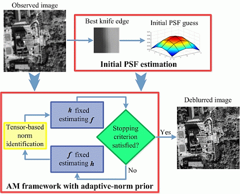

1. Introduction

Remote sensing images are often degraded in the acquisition process and are usually corrupted by blur. The blurring effect in remote sensing images is generally modeled by the total modulation transfer function (MTF), and it is caused by the cumulative effects of the optic instruments, the movement of the satellite during imaging, the environmental changes in outer space, and the scatter from particles in the atmosphere [1,2]. Instead of the MTF, the blur can also be modeled by the point spread function (PSF). The Fourier transform of the PSF is the total optical transfer function (OTF), and the MTF is the normalized magnitude of the OTF. The degradation process using the PSF is described as:

$$g=h*f+n$$

(1)

where * denotes the convolution operation. f and g represent the unknown sharp image and the observed image, which are the raw data without pre-focusing. h is the total shift-invariant atmospheric PSF of the remote sensing images, and is usually approximated by a Gaussian function [3–5]. n is the acquisition noise. According to whether h is available or not, the restoration methods can be classified into two types: (1) non-blind restoration when h is known; and (2) blind restoration when neither f nor h is completely given. In this paper, we focus on blind restoration to remove the blurring effect in remote sensing images, without measuring the MTF.

For a high-resolution on-orbit sensor, the blur can be derived from the degraded image or the scene itself by measuring man-made targets or typical features [6]. A great deal of effort has been made to improve the MTF measurement methods, which include the knife-edge method [7], the trap-based target method [7], and the pulse method [8]. Once the MTF is obtained, the remote sensing images can be restored by applying an MTF compensation (MTFC) technique [2,9] or other non-blind restoration methods [5,10–12]. Because knife edges can usually be found in remote sensing images near features like bridges, glaciers, buildings, and even shadows, the knife-edge method can be used for many remote sensing applications. However, a major concern of the knife-edge method is that the ground target sometimes needs to be slanted [13] and should have high fidelity to effectively represent the edge spread function (ESF) or the line spread function (LSF). Therefore, knife edges usually need to be manually selected and may not be ideal, or, in some cases, they may not exist. Previous studies have mainly focused on the extraction procedure of the MTF (or PSF), but the estimated MTF (or PSF) is often not very precise, and does not result in satisfactory results in the restoration procedure [5,7].

In the image processing field, blind restoration methods have been extensively explored, and detailed introductions to the existing blind restoration methods can be found in [14,15]. According to the blur identification stages, the blind restoration methods can be classified into two categories: (1) methods that estimate the PSF before the image is identified, as separate procedures [5,16–18]; and (2) methods that estimate the PSF and the image simultaneously in a joint procedure [19–33]. In our work, we mainly focus on the second type of method. Among this type of method, a strategy named alternating minimization (AM) has drawn considerable attention in recent years. AM was first proposed by You et al. [22], and the cost function can be expressed as:

$$C\left(f,h\right)={\Vert g-h*f\Vert }_2^2+\lambda R(f)+\gamma R(h)$$

(2)

where the first item ensures the fidelity between the observed image and the unknown sharp image. The last two items are the prior terms, which model the prior distributions of the unknown sharp image and the PSF, respectively. λ and γ are the corresponding regularization parameters which balance the tradeoff between the data fidelity term and the prior terms. After the prior types for the last two items are decided, iterative optimization procedures are employed to minimize Equation (2) with respect to f and h alternately to gradually achieve the global convergence.

Similar models have since been developed by the use of a total variation (TV) prior [23–25,31], a Huber-Markov random field (HMRF) prior [28], or a sparse prior [30,32]. The optimization methods have also developed from the steepest descent method, conjugate gradient (CG) [22,24,28,29], and Bregman iteration [25] to split Bregman [31] or augmented Lagrangian methods [32]. The straightforward AM framework has been proven to be competitive when compared to much more complicated methods [32,34], and is a good strategy to remove the blurring effect in images. However, whether with constraints on the PSF or not, Equation (2) is usually non-convex. Therefore, the AM framework needs a good initial PSF to promote the global convergence and a good criterion to stop the iteration in time [35]. To get a good initialization, shock filters [26] and edge detectors[30] have been used to enforce edges in images. In addition, several whiteness measures based on the residual image were designed in [35] to jointly estimate the parameter and stop the iteration of the AM framework.

As noted before, the implementation of the AM framework greatly depends on a good initial PSF, as well as a reasonable stopping criterion, and the performance of the knife-edge method is inevitably limited by the accuracy of the estimated MTF (or PSF). Therefore, in our work, an automatic blind restoration method is designed to quickly remove the blur in remote sensing images. The contributions of this work can be summarized as follows:

(1)

The AM framework is set up first to make the restoration process blind, and an automatic knife-edge detection method [5] is then used to extract the best knife edge. We then prove that the PSF estimated from the knife edges, although not very precise, is actually good enough to initialize the AM framework. Therefore, by combining the AM framework with the knife-edge method, the problems of the initial PSF in the AM framework and the unsatisfactory performance of the knife-edge method can both be solved.

(2)

To deal with the stopping problem of the AM framework, the feasibility of applying image quality indexes is discussed. Furthermore, an image sharpness index, which needs no reference, correlates well with the image quality, and shows little fluctuation, is proven to be a good stopping criterion for the AM framework.

(3)

An adaptive-norm prior based on the structure tensor is utilized in the AM framework, and it guarantees the global performance of the restoration. Preconditioned conjugate gradient (PCG) optimization is also implemented to ensure rapid iteration of the algorithm. In addition, we also investigate schemes to implement the proposed method with real data of a large size.

The rest of this paper is organized as follows. Details of the AM framework implementation and the optimization solution are presented in Section 2. Section 3 describes the initial PSF estimation procedure. Section 4 describes the automatic stopping criterion for the AM framework. Section 5 gives the computational cost analysis of the proposed method. Section 6 describes the experimental studies for verifying the proposed AM-KEdge method in both simulated and real data situations. Finally, a summary of our work is provided in Section 7.

2. AM Framework Modeling and Optimization

2.1. Adaptive-Norm Prior for the AM Framework

An important concern is the selection of the image and PSF constraints in Equation (2). The classical TV prior [23–26,31,36] can preserve the edges well, but aberrations occur when recovering smooth regions or weak edges; therefore, selective methods have been explored in recent years to obtain a solution to this shortcoming [37–40]. “Selective” means using different norms q (1 ≤ q ≤ 2) for different pixels. The key idea of the selective methods is to adapt different values of q at different points or regions, according to their spatial or textural characteristics. In light of the selective method in [38], we have developed a similar adaptive strategy, which is also pixel-wise.

The structure tensor based spatial property analysis used in [41] is first conducted to identify the spatial property of the blocks around each pixel. The structure tensor matrix is defined as:

$$S_{i,j}=\left({\nabla }_{i,j}f\right){\left({\nabla }_{i,j}f\right)}^T$$

(3)

where S_i,j is the structure tensor matrix in pixel (i,j). ${\nabla }_{i,j}f={\left[{\nabla }_{i,j}^{h}f,{\nabla }_{i,j}^{v}f\right]}^T$, with ${\nabla }_{i,j}^h$ and ${\nabla }_{i,j}^v$ representing linear operators of the first-order differences in the horizontal and vertical directions of pixel (i,j): ${\nabla }_{i,j}^{h}f=f\left(i,j+1\right)-f\left(i,j\right)$ and ${\nabla }_{i,j}^{v}f=f\left(i+1,j\right)-f\left(i,j\right)$. The noise in degraded images is also sensitive to the structure tensor, and the spatial structure information can be contaminated. Therefore, to represent the spatial property of each pixel accurately, the structure tensor is averaged to suppress the noise:

$${\overline{S}}_{i,j}=\frac{1}{9}\sum _{m=i-1}^{i+1}\sum _{n=j-1}^{j+1}{S}_{m,n}$$

(4)

where S̄_i,j is the average structure tensor, which is determined as the average of each pixel and its eight connected pixels. The spatial variance can be represented by the two eigenvalues of S̄_i,j, and the spatial property parameter δ_i,j at pixel (i,j) is further defined as:

$${\delta }_{i,j}=\left|e_{i,j}^1\right|+\left|e_{i,j}^2\right|$$

(5)

where $e_{i,j}^1$ and $e_{i,j}^2$ are two eigenvalues of S̄_i,j. A threshold value T is decided in advance, and all the pixels in an image can be classified into pixels from homogeneous regions (δ_i,j < T) or pixels from edges (δ_i,j ≥ T). The spatial property parameter δ_m,n in Equation (5) for all the pixels was normalized first, and then a fixed threshold T = 0.5 was used. After that, an adaptive-norm prior is used:

$$R(f)=\sum _{i,j}{\Vert \sqrt{{({\nabla }_{i,j}^{h}f)}^2+{({\nabla }_{i,j}^{v}f)}^2}\Vert }_{q_{i,j}}^{q_{i,j}}$$

(6)

In Equation (7)q_i,j is the norm used at pixel (i,j). For pixels from homogeneous regions (δ_i,j < T), we constrain them with an l₂ norm (q_i,j = 2). In contrast, for pixels from edges (δ_i,j ≥ T), an l₁ norm (q_i,j = 1) is used to preserve the edge information. The preceding expression is not differentiable when ${({\nabla }_{i,j}^{h}f)}^2+{({\nabla }_{i,j}^{v}f)}^2=0$. A more general smooth approximation is therefore used:

$$R(f)=\sum _{i,j}{\Vert \sqrt{{({\nabla }_{i,j}^{h}f)}^2+{({\nabla }_{i,j}^{v}f)}^2+\epsilon }\Vert }_{q_{i,j}}^{q_{i,j}}$$

(7)

where ɛ is a small positive parameter which ensures the differentiability.

The practical atmospheric PSF in remote sensing images is assumed to be a Gaussian-like shape, so the l₂ norm is more suitable for the PSF:

$$R(h)={\Vert Q*h\Vert }_2^2$$

(8)

where Q is a 2D Laplacian filter which penalizes the PSFs that are not smooth:

$$\left(\begin{array}{ccc}\hfill 0\hfill & \hfill -1\hfill & \hfill 0\hfill \\ \hfill -1\hfill & \hfill 4\hfill & \hfill -1\hfill \\ \hfill 0\hfill & \hfill -1\hfill & \hfill 0\hfill \end{array}\right)$$

(9)

Finally, we incorporate Equations (7) and (8) into Equation (2), and the final minimization cost function becomes:

$$C\left(f,h\right)={\Vert g-h*f\Vert }_2^2+\lambda \sum _{i,j}{\Vert \sqrt{{({\nabla }_{i,j}^{h}f)}^2+{({\nabla }_{i,j}^{v}f)}^2+\epsilon }\Vert }_{q_{i,j}}^{q_{i,j}}+\gamma {\Vert Q*h\Vert }_2^2 \hspace{1em}$$

(10)

2.2. Preconditioned Conjugate Gradient Optimization

To optimize Equation (10), the AM framework cycles between the step minimizing f while fixing h, and the step minimizing h while fixing f. For the f (or h) step, the PSF (or the image) is fixed as the output in the last h (or f) procedure. Therefore, by the use of a matrix-vector representation, the Euler-Lagrange equation of the energy function in Equation (10) can be expressed using the following system [42]:

$${\nabla }_{\mathbf{\text{f}}}C(\mathbf{\text{f}},\mathbf{\text{h}})={\mathbf{\text{H}}}^T(\mathbf{\text{Hf}}-\mathbf{\text{g}})+\lambda {\mathbf{\text{L}}}_{\mathbf{\text{f}}}\mathbf{\text{f}}$$

(11)

or

$${\nabla }_{\mathbf{\text{h}}}C(\mathbf{\text{f}},\mathbf{\text{h}})={\mathbf{\text{F}}}^T(\mathbf{\text{Fh}}-\mathbf{\text{g}})+\gamma {\mathbf{\text{Q}}}^T\mathbf{\text{Qh}}$$

(12)

Here, g, f, and h are the vector form of g, f, and h in lexicographical order. H, F, and Q are the matrix representation of h, f, and Q. H^T, F^T, and Q^T are the transposes of H, F, and Q. L_f is the matrix representation of the central difference of the following differential operator:

$$-q_{i,j}\nabla \cdot \left(\frac{\nabla }{{\left(\sqrt{{\left({\nabla }_{i,j}^{h}f\right)}^2+{\left({\nabla }_{i,j}^{v}f\right)}^2+\epsilon }\right)}^{2-q_{i,j}}}\right)$$

(13)

Because the operator L_f is highly nonlinear when q_i,j = 1, lagged diffusivity fixed-point iteration is used. This linearizes the term by lagging the diffusion coefficient one iteration behind:

$$1/\sqrt{{\left({\nabla }_{i,j}^{h}f\right)}^2+{\left({\nabla }_{i,j}^{v}f\right)}^2+\epsilon }$$

(14)

This strategy has been proven to converge globally and quickly, and readers are directed to [42] for more details. In the k th iteration, f^k (or h^k) can be calculated by solving the following linear system:

$$\left({\mathbf{\text{H}}}^T\mathbf{\text{H}}+\lambda {\mathbf{\text{L}}}_{\mathbf{\text{f}}}\right){\mathbf{\text{f}}}^k={\mathbf{\text{H}}}^T\mathbf{\text{g}}$$

(15)

or

$$\left({\mathbf{\text{F}}}^T\mathbf{\text{F}}+\gamma {\mathbf{\text{Q}}}^T\mathbf{\text{Q}}\right){\mathbf{\text{h}}}^k={\mathbf{\text{F}}}^T\mathbf{\text{g}}$$

(16)

To obtain a desirable H^TH + λL_f (or F^TF + γQ^TQ), a PCG method with a factorized banded inverse preconditioner (FBIP) [43] is used. The FBIP is a special case of the factorized sparse inverse preconditioner (FSIP) [44] and is employed to approximate H^TH + λL_f (or F^TF + γQ^TQ) so that Equation (15) (or (16)) can be quickly solved.

3. Initial PSF Estimation by the Use of Automatic Knife-Edge Detection

The AM framework needs a good initial PSF to guarantee global convergence and a relatively fast convergence speed. Thanks to the knife-edge method, a good initial PSF can be estimated for remote sensing images from the knife-edge features. Knife edges stimulate the imaging system at all spatial frequencies and are utilized to evaluate the spatial response [8]. The knife-edge detection method in [5] is used here to extract the best knife edges by detecting long, high-contrast straight edges that are homogenous on both sides. A PSF identification procedure is then carried out.

3.1. Extraction of the Best Knife Edge

Ideal knife edges rapidly transfer from one gray level to the opposite, so they are often found around edges. The edge detection method proposed in [5] is used to extract the best knife edges from remote sensing images. This method first employs the Canny edge detection algorithm [45] to extract the edge features, and the selection of the knife edges is then limited to only edges. The results of the Canny edge detector may be contaminated by neighborhood noise. Therefore, a two-stage framework is conducted to evaluate the straightness of the edges at both small and large scales. At the end of the large-scale evaluation, the kurtosis [46,47] of the pixels in the edges is calculated. The kurtosis can characterize the bi-modal property of knife edges because ideal knife edges often have high contrast and homogeneous textures on both sides. Therefore, the edge with the lowest kurtosis is identified as the center of the best knife edge. Finally, after a resampling process, the edge is rotated and the best knife-edge block can be obtained. An example of the best knife-edge detection process is shown in Figure 1.

3.2. PSF Identification

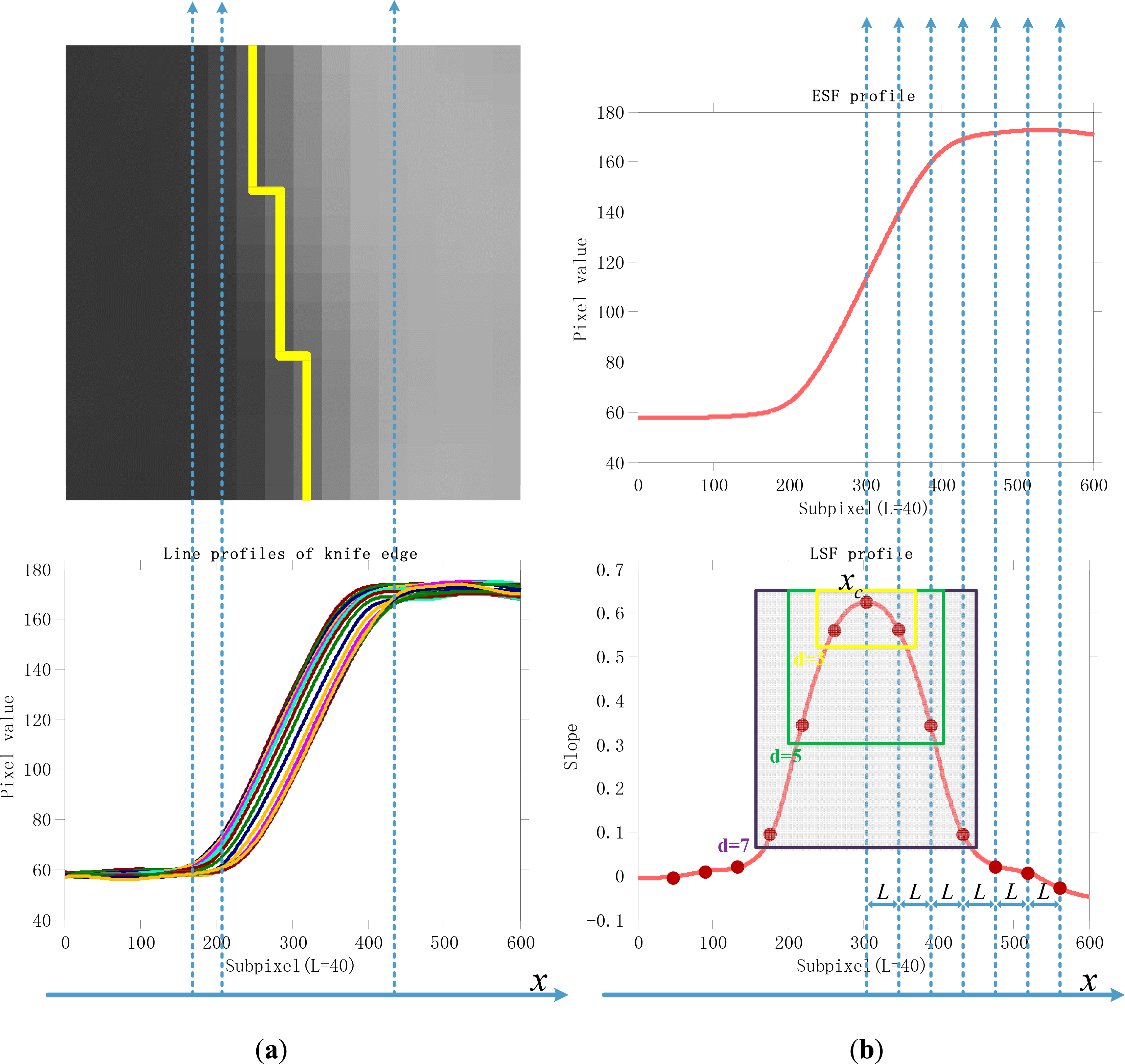
In our work, the practical PSF is approximated with a rectangular support region [28]. Given knife edges, the ESF and the LSF are estimated to calculate the PSF instead of the MTF. The lines of the knife-edge blocks are first averaged to get the ESF. The ideal edge is assumed to be a straight and vertical line. However, as the example in Figure 2a shows, the knife edge from an automatic procedure will be neither straight nor vertical at the pixel level, so the location of the edge should be further adjusted. Because the location of the edge is characterized by the maximum slope in a continuous line [8], all the lines are interpolated to build pseudo-continuous lines: L values between each data pair using a three-order spline interpolation. The subpixel locations of the maximum slope are found line by line and are fitted to be straight by least-squares fitting [8]. All the lines are then overlapped according to these locations and averaged, so an ESF at the subpixel level is obtained. The LSF is further calculated from the ESF by the use of a differentiation operation:

$$\mathit{LSF}(x)=\mathit{ESF}(x)-\mathit{ESF}(x-1)$$

(17)

The next stage is to estimate the PSF from the LSF. An example of the ESF and the corresponding LSF profile is presented in Figure 2b. The LSF at the subpixel level cannot be directly used to obtain the PSF and needs to be sampled at the pixel level. First, the center of the LSF must be identified. In the LSF profiles, the center should be near to the maximum value, and the profiles on the two sides should be the most symmetrical. For position x near the maximum, the subpixel LSF values are sampled every L points left and right, respectively. The differences between the two sides are then calculated:

$$\mathit{diff}\left(x\right)=\sum _{i=1}^2{\left(\mathit{LSF}\left(x+L\cdot i\right)-\mathit{LSF}\left(x-L\cdot i\right)\right)}^2$$

(18)

The position x_c with the minimum diff (x) is then selected as the center of the LSF. Secondly, the LSF size d and the values should be estimated. The average percentage of the two LSF boundary sample values with respect to the sum of the LSF values is calculated as:

$$\mathit{per}\left(d\right)=\frac{\frac{1}{2}\left(\mathit{LSF}\left(x_c-L\frac{d-1}{2}\right)+\mathit{LSF}\left(x_c+L\frac{d-1}{2}\right)\right)}{\sum _{x=0}^{d-1}\mathit{LSF}\left(x_c+L\left(x-\frac{d-1}{2}\right)\right)}$$

(19)

where $\mathit{LSF}\left(x_c-L\frac{d-1}{2}\right)$ and $\mathit{LSF}\left(x_c+L\frac{d-1}{2}\right)$ are the two boundary samples. Equation (19) is initialized with the minimum candidate d = 3 and increases by two each time, as shown in Figure 2b. When per(d) is lower than a threshold α, the candidate size d is believed to include the whole LSF. The LSF is then the sample points within d in order and normalized. Lastly, the PSF is estimated from the LSF. The isotropic blurring statistics of the remote sensing images through the atmosphere are assumed as in [5], thus, the LSF is an approximation of the PSF in any direction. A rectangular approximation of the PSF is calculated by expanding the normalized LSF to two dimensions. Further on in the AM process, we relieve the isotropic assumption to allow the PSF to be anisotropic. This is more practical in real situations, and a more accurate PSF can be refined.

4. Automatic Stopping Criterion for the AM Framework

The AM framework is performed by minimizing the f step and the h step separately and alternatively. Unfortunately, the AM framework can be inefficient, even with a good initial PSF from the best knife edge. As the AM moves on, an image with the best quality will appear [33], but if the optimization procedure is not stopped in time, the quality of the results will start to fall. However, when applying AM to real remote sensing images, it is difficult to identify when the image has the best quality because the convergence speed can be influenced by the strength of the regularization parameters. The AM framework also becomes more unstable when both the image and the PSF prior terms have parameters (λ and γ in Equation (10)) to be determined. In fact, the visual performance is mainly determined by the parameter of the image term λ, because it controls the tradeoff between the fidelity term and the image prior term. It is also in the f step that we restore the images to clearer ones. When λ is decided, the parameter of the PSF term γ should also be carefully selected. Too small a value will make the convergence speed slow, while too large a value cannot refine a more precise PSF, and the final restored results will be influenced.

To solve the stopping problem, in our work, we refer to an NR image quality assessment (IQA) index to serve as an automatic stopping criterion. NR IQA indexes aim to predict the human evaluation of image quality, without any access to a reference image. During the past decade, lots of NR IQA algorithms [48–52] have been proposed to evaluate the sharpness/blurring of images. Some of the indexes have been proven to be effective in capturing the blurring effect on the perceived sharpness, and can even achieve comparative results to some full-reference (FR) IQA indexes, which are usually more accurate. In [52], a novel NR image sharpness assessment method called the local phase coherence-based sharpness index (LPC-SI) was proposed. The LPC-SI considers the sharpness as strong local phase coherence (LPC) [53] near distinctive image features evaluated in the complex wavelet transform domain, and calculates the LPC at arbitrary fractional scales [52].

Given an image f, it is first passed through a series of N-scale M-orientation log-Gabor filters without any subsequent downsampling process. The LPC strength at the j th orientation and the k th spatial location is then calculated as $S_{\mathit{LPC}}^{\left\{j,k\right\}}$. The LPC strength is further combined at each spatial location by a weighted average across all the orientations by:

$$S_{\mathit{LPC}}^{\left\{k\right\}}=\frac{{\sum }_{j=1}^M\left|c_{1jk}\right|S_{\mathit{LPC}}^{\{j,k\}}}{{\sum }_{j=1}^M\left|c_{1jk}\right|+C}$$

(20)

where M is the number of orientations, c_1jk is the first (finest) scale coefficient at the j th orientation and the k th spatial location, and C is a constant to avoid instability. The overall LPC-SI is calculated using a weighted averaging method based on the ranked LPC values as:

$$S_{\mathit{LPC}}=\frac{{\sum }_{k=1}^K-\left(\frac{k-1}{K-1}\right)S_{\mathit{LPC}}^{\left\{\left(k\right)\right\}}/{\beta }_k}{{\sum }_{k=1}^K\text{exp}\left(-\left(\frac{k-1}{K-1}\right)/{\beta }_k\right)}$$

(21)

where K is the number of spatial locations, and $S_{\mathit{LPC}}^{\left\{\left(k\right)\right\}}$ stands for the sorted LPC strength values which satisfy $S_{\mathit{LPC}}^{\left\{\left(1\right)\right\}}\ge S_{\mathit{LPC}}^{\left\{\left(2\right)\right\}}\ge \cdots \ge S_{\mathit{LPC}}^{\left\{\left(K\right)\right\}}$. The parameter β_k controls the decay speed of the weights.

Compared with other NR IQA algorithms [48–51], LPC-SI correlates better with image sharpness and shows less fluctuation with the iterations. Its computational load is also acceptable. Therefore, the LPC-SI is used as the stopping criterion in our work. In our later experiments, we show that the LPC-SI has a similar performance to the FR peak signal-to-noise ratio (PSNR) and the structural similarity (SSIM) indexes [54] and it is stable enough to form an automatic criterion to stop the iteration of the AM framework. In our experiments, λ was first determined manually, and a moderate γ was further decided according to λ. The AM procedure starts by fixing λ and γ. The LPC-SI of f at the end of each iteration is calculated using Equation (21), and the AM is stopped automatically as soon as the LPC-SI starts to fall.

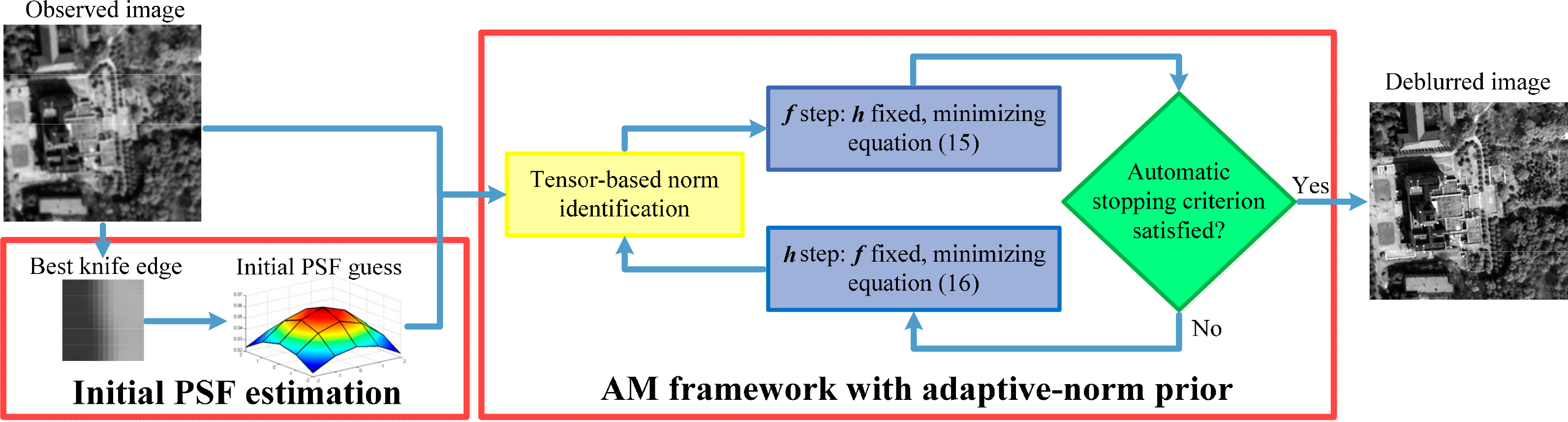
Finally, the whole proposed AM-KEdge method, combining the automatic knife-edge detection technique and the AM framework, is illustrated in Figure 3.

5. Computational Cost Analysis

To determine the cost of the proposed AM-KEdge method, we implemented the algorithm in MATLAB with C/MEX functions and tested it on a laptop with an Intel Core i7-3517U processor. For images of 300 × 300, the initial PSF estimation process took 10 s on average. In the AM stage, one f step took about 7 s (400 iterations in each loop) and one h step about 0.5 s (800 iterations in each loop). The time taken to calculate LPC-SI one time was 1 s. The number of iterations in the main loop averaged about 10 times. Therefore, the total restoration time for images of 300 × 300 was about 95 s.

Another issue is that real remote sensing images are of a large size (for example 5200 × 5200), and an iterative method would have a high computational burden. This problem can be tackled using the following two schemes:

(1)

Two-stage scheme: In our work, the blur is assumed to be shift-invariant. Therefore, the PSF in all the parts of the image are the same. When the size of images is very large, we can select a small patch (for example 300×300) with edge features. In the first stage, the parameters λ and γ in Equation (10), together with the best iteration number n, can both be identified on the small patch. At the second stage, we start the iterations using parameters from the first stage. In the first n−1 iterations, the AM is processed only on the small patch. The whole image is only processed in the last (nth) iteration using the estimated PSF from the (n−1)th iteration on the small patch. The reason why this scheme can be implemented is that the usable outputs of the first stage are the PSFs and not the restored small patches. This scheme was proven to be successful with the AM framework in [55].

(2)

Pyramid scheme: This scheme can be useful when the data size is not very large or the PSF size is relatively large. The images and the PSF are both scaled down until the PSF size is 3 × 3 pixels. The AM is started at the lowest scale, and the results are then upsampled for the next scale. When the scale is upsampled to the original size, we start to calculate the LPC-SI, and the iteration stops as soon as the LPC-SI falls. This scheme was proven to significantly speed up the AM framework in [34].

6. Experimental Results

The restoration performance of the proposed AM-KEdge method was verified in both simulated and real data experiments. Three blind restoration methods were compared: the marginal likelihood optimization (MLO) method [56] and two AM methods (AM with a sparse prior (AM-Sparse) [30] and AM with a HMRF prior (AM-HMRF) [28]). For the five MLO methods in [56], a sparse mixture of a Gaussian (MOG) prior in the filter domain was used to yield the best results. For the AM-Sparse method, the cyclic boundary conditions were used, and the unknown boundary was not considered in the experiments.

The initial PSFs for MLO and AM-HMRF were manually set the same as the degraded image, for fairness. AM-Sparse assumes a limited size of the PSF and only needs to initialize the PSF size. It can also be initialized by gradually decreasing the sparsity parameter in the iterations in the first few steps. AM-KEdge can be initialized automatically by the use of the best knife edge and does not need to be manually set. For the automatic knife-edge detection method in [5], the size of the Gaussian filter at a large scale was set as 16 × 16, and the window size to calculate the kurtosis was 7 × 7 in all the experiments. In the PSF identification stage, the interpolation number L between each pixel pair was fixed at 40, and the threshold α to decide the PSF size in Equation (19) was fixed at 0.1.

In the AM stage of AM-KEdge, the number of iterations in one f step and h step were 400 and 800, respectively. λ and γ in Equation (10) were set manually and then fixed, with the values in the region of 10⁻²–10⁻¹ and 10⁶–10⁷. The final results of the AM framework can be different according to the various stopping criterions. For AM-Sparse, it was stopped automatically by the use of the whiteness measure $M_R^l$ in [35], as the authors did in the released code [30]. AM-HMRF was stopped when the relative variation of the image was less than a predetermined threshold [28]. AM-KEdge was stopped automatically by the proposed automatic stopping criterion by the use of the LPC-SI.

To evaluate the quality of the restored images, two FR and two NR indexes were employed in the simulated and real data experiments, respectively. The peak signal-to-noise ratio (PSNR) and structural similarity (SSIM) [54] can be calculated when a reference image is given, so they were used in the simulated experiments. The metric Q [49] and LPC-SI can reflect the sharpness of images without the use of a reference image, so they were used in the real data experiments, to give the quantitative results. With a maximum value of 255 in all our experiments, the metrics are defined as:

$$\mathit{PSNR}=10{\text{log}}_{10}\left(\frac{{255}^2}{{\Vert \widehat{f}-f\Vert }^2}\right)$$

(22)

$$\mathit{SSIM}=\frac{\left(2{\mu }_f{\mu }_{\widehat{f}}+C_1\right)\left(2{\delta }_{\widehat{f}f}+C_2\right)}{\left({\mu }_f^2+{\mu }_{\widehat{f}}^2+C_1\right)\left({\delta }_f^2+{\delta }_{\widehat{f}}^2+C_2\right)}$$

(23)

$$Q=s_1\frac{s_1-s_2}{s_1+s_2}$$

(24)

where f̂ and f are the restored image and the high-quality reference image, and their mean intensities are given by μ_f̂ and μ_f. δ_f̂, δ_f, and δ_f̂f represent the standard deviation of the restored image, the high-quality reference image, and their covariance, respectively. C₁ and C₂ are both constants. s₁ and s₂ model two singular values of each 8 × 8 block in the gradient matrix of the restored image, and the final metric Q can be calculated as the average of all the anisotropic patches.

In addition, the normalized mean square error (NMSE) between the true and restored PSF was also calculated to evaluate the quality of the PSF in the simulated experiments:

$$\mathit{NMSE}=\frac{{\Vert \widehat{h}-h\Vert }^2}{{\Vert h\Vert }^2}$$

(25)

where ĥ and h are the restored PSF and the true PSF.

6.1. Simulated Restoration Experiments

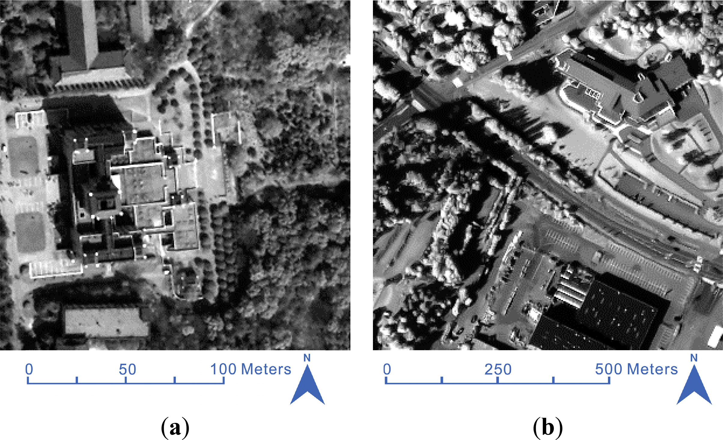
Figure 4 presents the two preprocessed 300 × 300 remote sensing images used in the simulated experiments. The images were cropped from high-quality QuickBird and SPOT products, respectively. We tested all the methods in both noise-free and noisy cases. The atmospheric PSF of remote sensing images is usually approximated by a Gaussian function [3–5], thus, we simulated the blurring effect by the use of a truncated Gaussian PSF approximated with a rectangular support region in the simulated experiments. We also made the assumption that the noise in remote sensing images is usually not serious, and, therefore, a moderate level of noise was added in the simulated experiments. In the noise-free case, the blurred images were generated by convoluting the test images and a 5 × 5 truncated Gaussian PSF with a standard deviation of 2, as shown in Figures 5a and 6a. Figures 7a and 8a illustrate the blurred and noisy images in the noisy case, by further adding white Gaussian noise (WGN) with a variance of 3 to the blurred images in Figures 5a and 6a. MLO and AM-HMRF were initialized by the use of a 5 × 5 truncated Gaussian PSF with a standard deviation of 1.5 in the simulated experiments. In addition, for all the methods, the parameters were manually adjusted to yield the best PSNR and SSIM values and superior visual results.

Table 1. Peak signal-to-noise ratio (PSNR), structural similarity (SSIM), and normalized mean square error (NMSE) results, and the computation times in the simulated experiments.

Images	Indexes	Degraded	MLO	AM-Sparse	AM-HMRF	AM-KEdge
Noise-free QuickBird	PSNR	22.8044	30.4897	31.2361	31.8142	32.8507
	SSIM	0.7328	0.9405	0.9545	0.9567	0.9651
	NMSE		0.0587	0.0326	0.0305	0.0286
	Time (s)		45.24	342.64	563.01	107.40
Noise-free SPOT	PSNR	20.3221	25.1873	28.8229	26.2813	29.2588
	SSIM	0.6873	0.8675	0.9548	0.8797	0.9516
	NMSE		0.0574	0.0299	0.0523	0.0238
	Time (s)		40.75	368.50	244.27	76.68
Noisy QuickBird	PSNR	22.6879	25.5439	24.0974	25.4393	26.3797
	SSIM	0.7164	0.8477	0.7874	0.8259	0.8629
	NMSE		0.1276	0.1597	0.1180	0.0689
	Time (s)		43.16	118.23	181.87	90.98
Noisy SPOT	PSNR	20.2569	22.4907	21.4175	22.8578	23.5138
	SSIM	0.6727	0.7985	0.7669	0.7855	0.8345
	NMSE		0.1749	0.2071	0.0906	0.0589
	Time (s)		41.11	142.00	175.25	95.05

shows the PSNR, SSIM, and NMSE values, and the computation times obtained in both the noise-free and noisy cases. For the restored images, in the noise-free case, the PSNR and SSIM results of all the methods are improved significantly with the QuickBird images. When applying these methods to the noise-free SPOT images, the results of MLO and AM-HMRF are limited, while AM-Sparse and AM-KEdge can still achieve PSNR and SSIM improvements. In the noisy case, the performance of all the methods is limited to a certain extent. Compared to the noiseless case, the performance of AM-Sparse is particularly influenced by noise in both the QuickBird and SPOT images. However, AM-KEdge can still achieve PSNR and SSIM improvements that surpass all the other methods. For the PSF, AM-KEdge can achieve the lowest NMSE values in all cases, which means that the final restored PSF of AM-KEdge is closest to the true one. In addition, with regard to the computation times, MLO has the least time cost among all the methods. For the AM-type methods, AM-KEdge is the fastest method, but is still double the time of MLO. However, by the use of a good initial PSF estimation and PCG optimization, the computation time of AM-KEdge is much faster than AM-Sparse and AM-HMRF. In the overall assessment in Table 1, the AM-KEdge method has an acceptable computational cost and achieves the highest PSNR and SSIM values and the lowest NMSE values in both the noise-free and noisy cases.

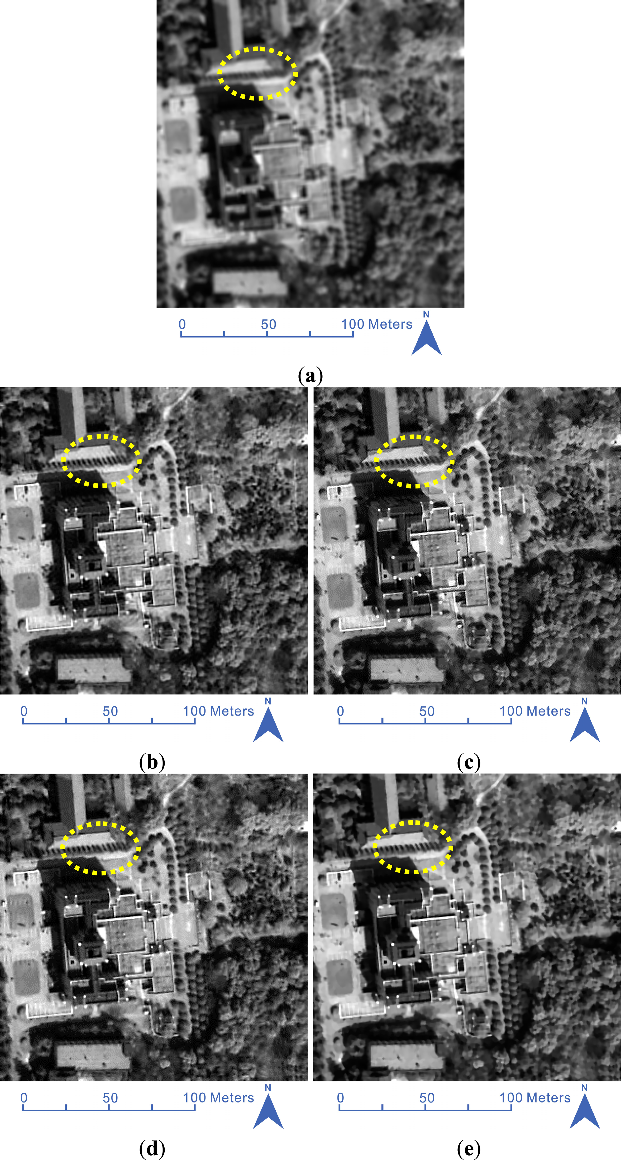
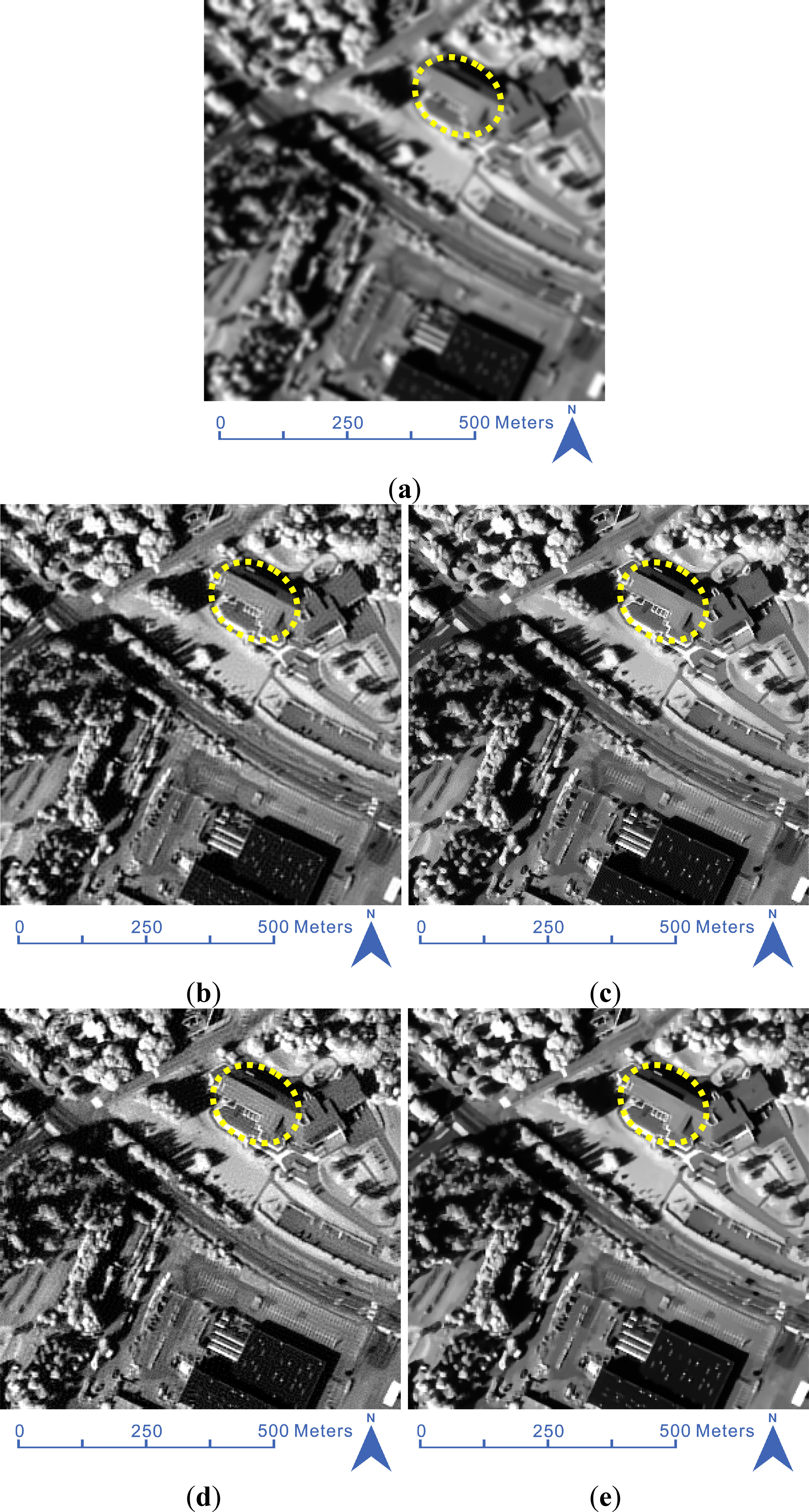
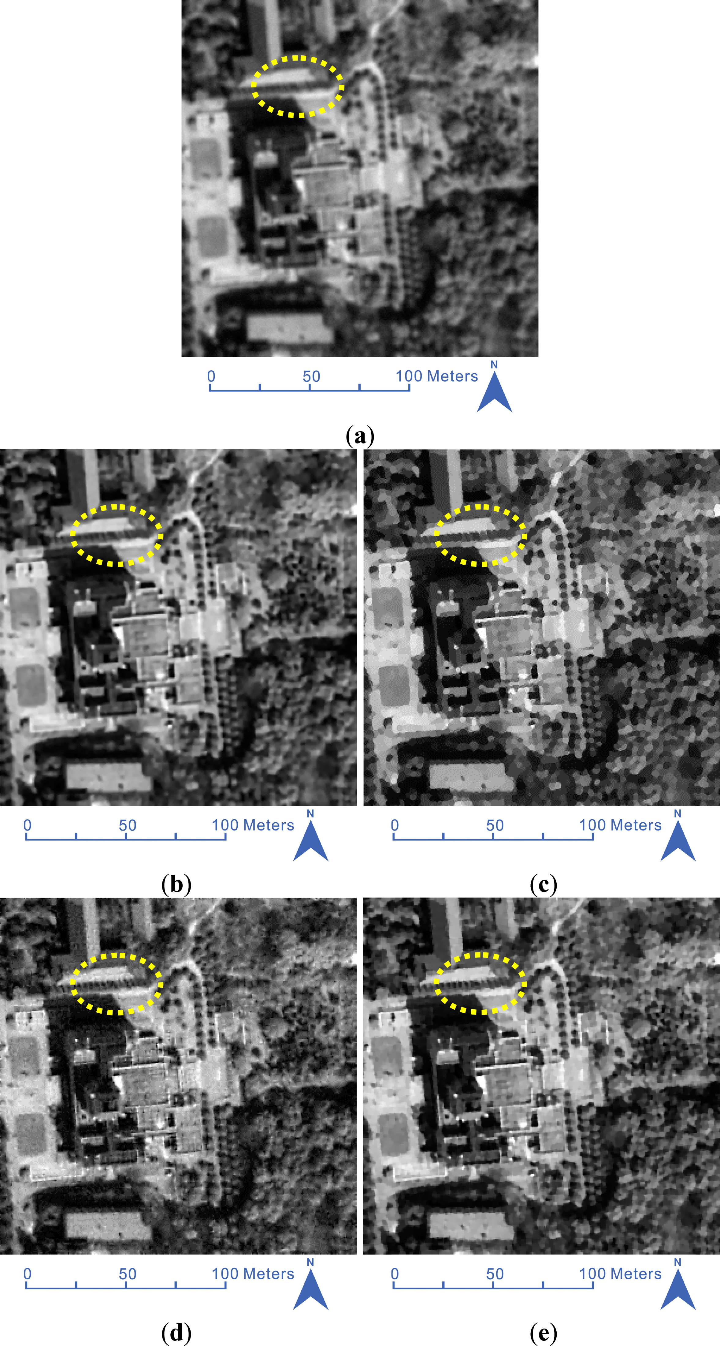
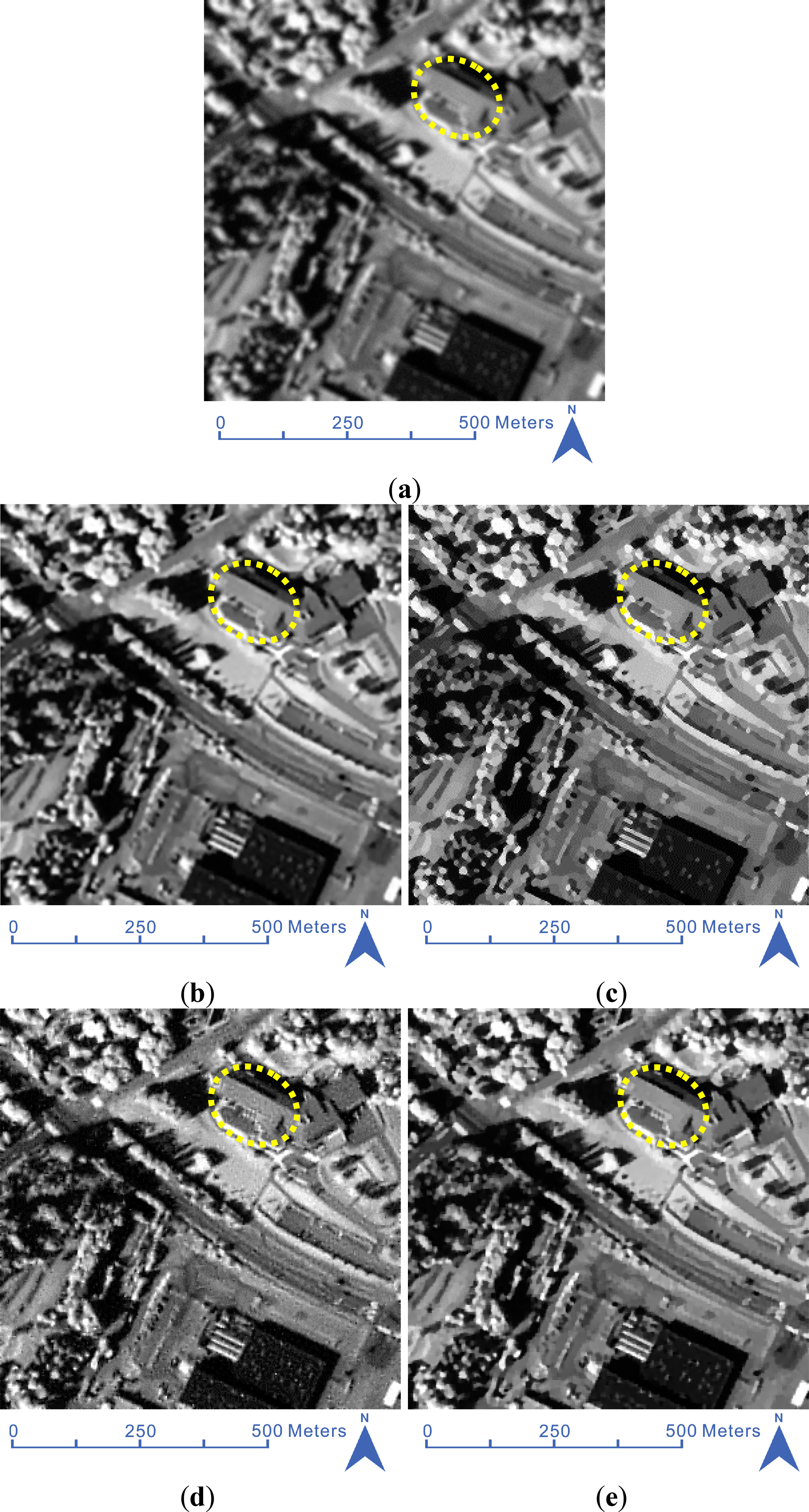
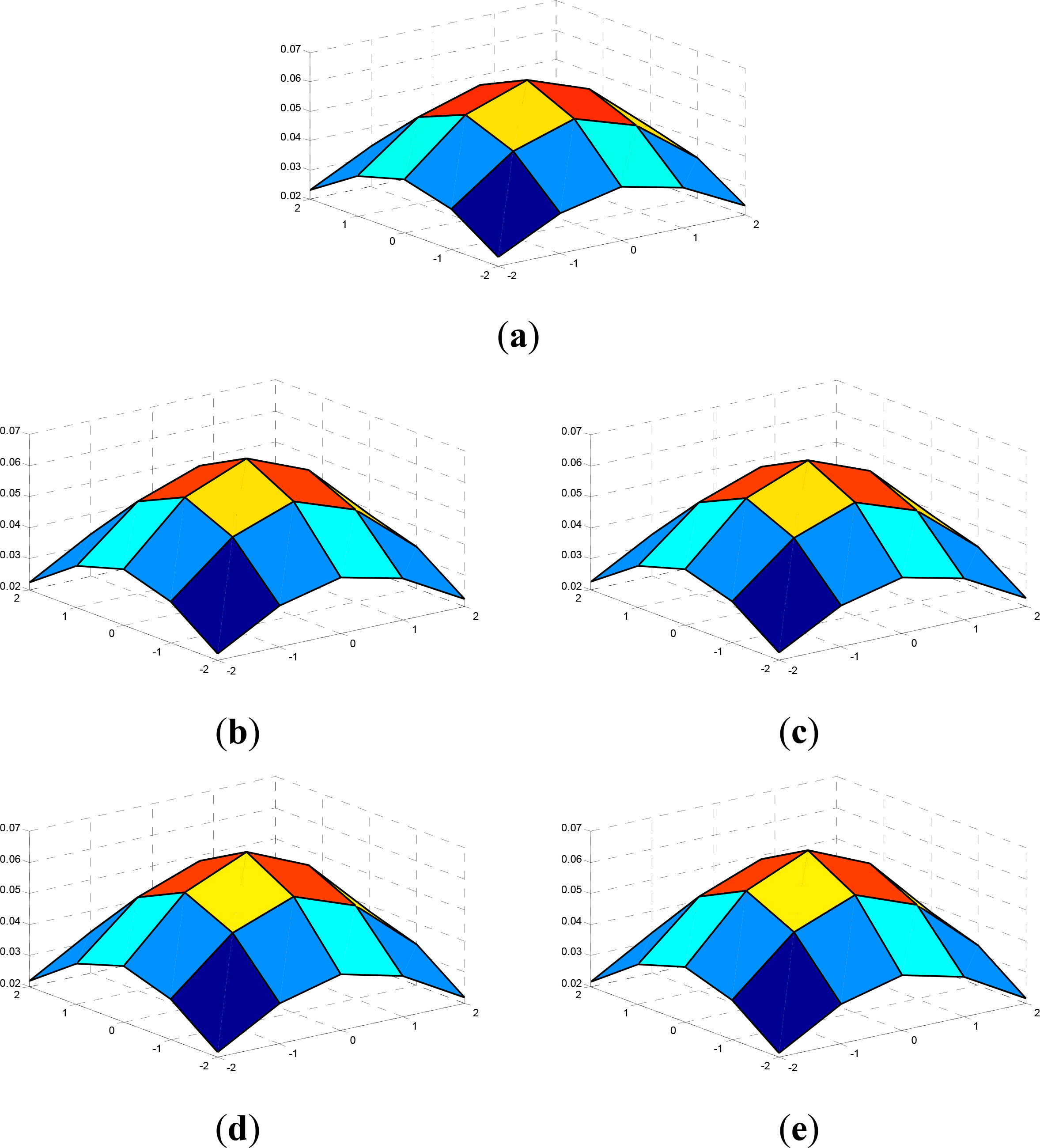
Visual comparisons of the results are presented in Figures 5 and 8. The MLO results are relatively stable in both the noise-free and noisy cases; however, the edges are not that clear and some “artifacts” are found near the edges in Figures 5–8b. The results of AM-Sparse differ according to the noise. With noise, the edge information is confused and the edge-sparsifying regularization fails to estimate more edges. Therefore, the restoration results with noise in Figures 7–8c have a somewhat “patchy” look, as discussed by the authors in [30]. For the results of AM-HMRF in Figures 5–8d, it can be concluded that the HMRF prior can preserve the edges well in all the results, but the noise degradation cannot be effectively controlled in the noisy case. In contrast, from the results of AM-KEdge in Figures 5–8e, we can see that the adaptive-norm prior produces sharper and clearer edges and more natural textures, regardless of the existence of noise. Therefore, the adaptive-norm prior used in the AM framework can strike a better balance between preserving the edge information and suppressing the noise, and is superior to the other priors. Moreover, in Figure 9, the final PSFs of AM-KEdge are compared with the true PSF (a 5 × 5 truncated Gaussian blur with a standard deviation of 2). It can be seen that regardless of noise, the final PSFs of AM-KEdge are close to the true one in all the experiments, which further confirms the good restoration results of AM-KEdge.

The kurtosis maps of degraded images Figures 5–8a are displayed in Figure 10. The kurtosis information is derived to model the bi-modal characteristics of the edges at a large scale. In Figure 10, lower kurtosis values represent higher length and straightness, and it is clear that the main edges are preserved in both the noise-free and noisy cases, due to the reasonable preprocessing at the small and large scales. Moreover, it can be seen that although the pixel values fluctuate when introducing noise in the experiments, the best knife edges can still be located accurately, as shown in Figures 10c–d. Additionally, the centers of the best knife edges are highlighted by circles in Figure 10, and they are (70,17), (136,52), (70,17), and (193,63), respectively. Comparing the centers of Figure 10b,d, we can see that the existence of noise can influence the selection of the best knife edges. However, the estimated initial PSFs are similar to using the extracted “best” knife edges, respectively. This means that good knife edges may not be unique, and the automatic PSF procedure is robust to noise, to a certain extent.

Figure 11 shows the evolution of the PSNR, SSIM, and LPC-SI values with the iterations in all the experiments. Here, the PSNR values are normalized to allow comparisons with the other two indexes. It is clear that for our restoration purpose, the evolution of the LPC-SI correlates well with that of the PSNR and SSIM in both the noise-free and noisy cases, and it is good enough to form an automatic stopping criterion when reference images are unavailable for real blurred remote sensing images.

To verify the effectiveness of the proposed PSF estimation method and to confirm the importance of a good initial PSF guess, we further compared the results of AM-KEdge with the results of the AM framework initialized by different manually selected initial PSFs (a 5 × 5 truncated Gaussian PSF with a standard deviation of 1.2, 1.5, and 3.0). In each experiment, the regularization parameters λ and γ were fixed the same as the best parameters in the previous experiments with the same degraded image for all the initial PSFs. The other factors that can affect the convergence speed were therefore controlled. We used “Knife,” “Std 1.2,” “Std 1.5,” and “Std 3.0” to distinguish the different initializations.

The evolution of the SSIM and PSNR values with the iterations for Figures 5–8a are summarized in Figures 12 and 13. It can be seen that the SSIM and PSNR values grow with the iterations in all cases. In both the noise-free and noisy images, AM-KEdge obtains the maximum SSIM and PSNR values after iterating only a few times, and the results have higher SSIM and PSNR values. In contrast, the AM framework initialized with the other initial PSFs takes more iterations to obtain convergent results, and it cannot achieve higher SSIM and PSNR values than initialization with the proposed method. In addition, in Figures 12 and 13, we mark the stopping positions automatically determined by the proposed LPC-SI-based stopping criterion with circles. The stopping positions for the images in Figures 5–8a are 12, 8, 10, and 11 times, respectively. It is clear that the AM framework stops at positions where the SSIM and PSNR values are close to the maximum, with fewer iterations. In addition, in Figures 12 and 13, it can be seen that with other initial PSFs, the AM framework can also gradually adjust itself into a convergent direction. However, the experimental results validate that the AM framework can be accelerated to obtain better results by combining it with an automatic knife-edge detection method. In addition, with the stopping criterion based on the sharpness index, the AM framework can be stopped automatically near the restored results with the best visual quality.

In fact, even if the estimated initial PSF is close to the true one in shape, it can still greatly influence the quality of the restored results. To give an intuitive illustration of the evolution of the PSF in the AM process, the NMSE values with the iterations for Figures 5–8a are also presented in Figure 14. It can be seen that whether initialized with the proposed PSF estimation method or a different manually selected initial PSF, the NMSE gradually decreases with the iterations and then increases again. However, it is interesting to note that the minimum points are not the positions where the SSIM and PSNR values are the highest in Figures 12 and 13. When the PSF with the iterations is closest to the true PSF, we cannot restore images with the best quality. Therefore, the true PSF is not the desired one that can achieve the best restoration results. The reason for this may be that any standard image in simulated experiments is more or less blurred, which makes the “true” PSF change a little.

Other than a good PSF initialization, the PCG used in our work could further improve the convergence speed in one AM loop. Figure 15 shows the convergence rate between PCG (with preconditioners) and CG (without preconditioners) on Figure 5a. Both PCG and CG are initialized with the proposed PSF estimation method and use the same settings as precious experiments. The evolution of the relative residuals in the first f step is presented as an example. It is clear that PCG converges faster than CG.

6.2. Restoration of Real ZY-3 Panchromatic Images

The Zi Yuan 3 (ZY-3) cartographic satellite was launched on 9 January 2012, and is China’s first civil high-resolution stereo mapping satellite. It carries four optical cameras: a panchromatic time delay integration charge coupled device (TDI-CCD) camera in the nadir view, two panchromatic TDI-CCD cameras in the forward and afterward views, and an infrared multispectral scanner (IRMSS). In the real data experiment, we tested the forward camera. This has a resolution of 3.5 m, a swath width of 52 km, and an on-orbit MTF value at the Nyquist frequency tested of more than 0.12 [57]. To prevent other pre-focusing influences, we used a full raw panchromatic image provided by the China Centre for Resources Satellite Data and Application (CRESDA). The image is level-0 data acquired on 11 January 2012, in Dalian City, Liaoning province, with a latitude and longitude of 39°N and 121.70°E, respectively. The full raw panchromatic image has a large size of 4096 × 4096, so we selected representative features to get eight 256 × 256 real blurred sub-images for convenience. For MLO and AM-Huber, a 5 × 5 truncated Gaussian PSF with a standard deviation of 0.9 was set as the initial PSF guess in all the experiments. For AM-Sparse, a PSF size of 3 × 3 or 5 × 5 was used. In

Table 2. Metric Q and local phase coherence-based sharpness index (LPC-SI) results and the computation times in the real data experiments.

Images	Indexes	Degraded	MLO	AM-Sparse	AM-HMRF	AM-KEdge
1	Metric Q	53.1422	64.9129	57.2741	68.6503	74.4053
	LPC-SI	0.9016	0.9394	0.9203	0.9475	0.9580
	Time (s)		27.96	94.88	260.21	51.32
2	Metric Q	62.0644	81.0123	70.0181	89.3713	95.5269
	LPC-SI	0.9173	0.9564	0.9320	0.9637	0.9737
	Time (s)		26.70	86.76	326.01	68.12
3	Metric Q	54.3968	74.3082	64.1530	81.2716	93.6372
	LPC-SI	0.9003	0.9380	0.9292	0.9420	0.9572
	Time (s)		25.02	106.31	275.13	70.44
4	Metric Q	53.3197	69.3859	62.1707	71.4048	81.8848
	LPC-SI	0.8683	0.9260	0.9076	0.9305	0.9572
	Time (s)		26.37	110.90	301.60	55.29
5	Metric Q	47.7225	61.0146	51.8822	66.6765	75.6365
	LPC-SI	0.8958	0.9401	0.9447	0.9430	0.9625
	Time (s)		26.10	113.86	224.50	79.20
6	Metric Q	41.5592	51.9965	44.5010	56.5267	58.1827
	LPC-SI	0.9124	0.9383	0.9277	0.9394	0.9628
	Time (s)		26.42	99.59	311.57	61.15
7	Metric Q	46.7506	62.3031	48.4182	64.7870	77.4521
	LPC-SI	0.8960	0.9318	0.9102	0.9313	0.9663
	Time (s)		25.49	63.23	307.01	51.52
8	Metric Q	50.8506	64.0524	54.1975	67.9792	72.8020
	LPC-SI	0.8879	0.9396	0.9480	0.9466	0.9556
	Time (s)		27.92	93.69	298.46	50.05

, the computation times and the metric Q and LPC-SI results of the real images are presented. Clearly, the proposed method achieves considerable metric Q and LPC-SI improvements over the other methods in all the experiments. MLO and AM-HMRF can also achieve metric Q and LPC-SI improvements with all the images. However, the performance of AM-Sparse was limited in most of the experiments. The reason for this is that it is sensitive to noise and is probably not suitable for real remote sensing images. The computation time of MLO was again the lowest in the real data experiments, while AM-KEdge took 50–80 s to restore a 256 × 256 sub-image.

Comparisons between the original cropped sub-images and the corresponding deblurred versions by AM-KEdge are presented in Figure 16. From Figure 16a–d,i–l, we can see that, in all cases, the original ZY-3 panchromatic images are blurred to some extent by various degradation factors. In Figure 16e–h,m–p, the restored results by AM-KEdge are shown. These images all have a higher visual quality than the original sub-images. The images are much sharper and more visible details are restored, and the blurring effect in the original sub-images is removed. The final PSFs of AM-KEdge for all the real data experiments are shown in Figure 17, and it is clear that the shape of the PSFs is roughly Gaussian-like, and the identified PSF support regions are small in size.

7. Conclusions

This paper has presented a new blind method for the restoration of remote sensing images. An automatic PSF estimation procedure utilizing knife-edge features was developed and the PSF initialization problem for the AM framework has been relieved. An NR sharpness index was used as the stopping criterion and was proven to stop the iterations of the AM framework close to the best quality. In addition, an adaptive-norm prior with PCG optimization was employed to ensure a comparative restoration performance and a fast convergence speed.

In our work, both simulated and real blurred remote sensing images were examined. The experimental results demonstrate that the proposed AM-KEdge method prevents the initial PSF problem, it achieves a highly competitive performance in comparison with other blind restoration methods [28,30,56], and it can stop automatically, close to the best visual quality. The computation cost and the solutions on images of large size are also discussed. Furthermore, in the simulated experiments, the necessary AM loops to achieve the best restoration results were reduced to only 10–15 times by the use of a good initial PSF. In addition, the preconditioner for CG reduces the computation time of each AM loop by about 20%. The unnecessary AM loops are therefore prevented soon after the quality of the restoration results falls, using the stopping criterion. An adaptive-norm prior based on structure tensor analysis guarantees the good performance of the final restoration results, with respect to both quantitative assessment and visual quality. The real data experiments with raw ZY-3 panchromatic images further validate the effectiveness of the proposed method, which performed well in all the experiments, while only taking 50–80 s.

However, the proposed AM-KEdge method imposes specific priors over the PSF according to the remote sensing degradation characteristics. The initial PSF estimation also relies on the existence of knife-edge features, which may not exist in some natural images. Furthermore, in our work, the support region of the PSF for real remote sensing images was modeled by a rectangular approximation, while other shapes might also be possible. We further verified that a small support region is suitable for ZY-3 panchromatic images, but this might not be the case for other sensors. Therefore, our future work will focus on PSF models for different sensors, and the application of the proposed method with data from other sensors.

References

- Leger, D.; Viallefont, F.; Hillairet, E.; Meygret, A. In-flight refocusing and MTF assessment of SPOT5 HRG and HRS cameras. Proc. SPIE 2003. [Google Scholar] [CrossRef]
- Li, X.; Gu, X.; Fu, Q.; Yu, T.; Gao, H.; Li, J.; Liu, L. Removing atmospheric MTF and establishing an MTF compensation filter for the HJ-1A CCD camera. Int. J. Remote Sens 2013, 34, 1413–1427. [Google Scholar]
- Savakis, A.E.; Trussell, H.J. Blur identification by residual spectral matching. IEEE Trans. Image Process 1993, 2, 141–151. [Google Scholar]
- Sheppard, D.G.; Hunt, B.R.; Marcellin, M.W. Iterative multiframe superresolution algorithms for atmospheric-turbulence-degraded imagery. J. Opt. Soc. Am. A 1998, 15, 978–992. [Google Scholar]
- Shacham, O.; Haik, O.; Yitzhaky, Y. Blind restoration of atmospherically degraded images by automatic best step-edge detection. Pattern Recogn. Lett 2007, 28, 2094–2103. [Google Scholar]
- Jalobeanu, A.; Zerubia, J.; Blanc-Feraud, L. Bayesian estimation of blur and noise in remote sensing imaging. In Blind Image Deconvolution: Theory and Applications; Campisi, P., Egiazarian, K., Eds.; CRC Press: Boca Raton, FL, USA, 2007; pp. 239–275. [Google Scholar]
- Ryan, R.; Baldridge, B.; Schowengerdt, R.A.; Choi, T.; Helder, D.L.; Blonski, S. IKONOS spatial resolution and image interpretability characterization. Remote Sens. Environ 2003, 88, 37–52. [Google Scholar]
- Choi, T. IKONOS Satellite on Orbit Modulation Transfer Function (MTF) Measurement Using Edge and Pulse Method. Master’s Thesis, South Dakota State University, Brookings SD, USA. 2002. [Google Scholar]
- Mu, X.; Xu, S.; Li, G.; Hu, J. Remote sensing image restoration with modulation transfer function compensation technology in-orbit. Proc. SPIE 2013. [Google Scholar] [CrossRef]
- Wiener, N. Extrapolation, Interpolation, and Smoothing of Stationary Time Series: With Engineering Applications; MIT Press: New York, NY, USA, 1964. [Google Scholar]
- Richardson, W.H. Bayesian-based iterative method of image restoration. J. Opt. Soc. Am. A 1972, 62, 55–59. [Google Scholar]
- Lucy, L.B. An iterative technique for the rectification of observed distributions. J. Astrophys 1974, 79, 745–754. [Google Scholar]
- Hwang, H.; Choi, Y.-W.; Kwak, S.; Kim, M.; Park, W. MTF assessment of high resolution satellite images using ISO 12233 slanted-edge method. Proc. SPIE 2008. [Google Scholar] [CrossRef]
- Kundur, D.; Hatzinakos, D. Blind image deconvolution. IEEE Signal. Process. Mag 1996, 13, 43–64. [Google Scholar]
- Bishop, T.; Babacan, S.; Amizic, B.; Katsaggelos, A.; Chan, T.; Molina, R. Blind. Image Deconvolution: Problem Formulation and Existing Approaches; CRC Press: Boca Raton, FL, USA, 2007. [Google Scholar]
- Cannon, M. Blind deconvolution of spatially invariant image blurs with phase. IEEE Trans. Acoust. Speech Signal. Process 1976, 24, 58–63. [Google Scholar]
- Chang, M.M.; Tekalp, A.M.; Erdem, A.T. Blur identification using the bispectrum. IEEE Trans. Signal. Process 1991, 39, 2323–2325. [Google Scholar]
- Reeves, S.J.; Mersereau, R.M. Blur identification by the method of generalized cross-validation. IEEE Trans. Image Process 1992, 1, 301–311. [Google Scholar]
- Ayers, G.; Dainty, J.C. Iterative blind deconvolution method and its applications. Opt. Lett 1988, 13, 547–549. [Google Scholar]
- Jefferies, S.M.; Christou, J.C. Restoration of astronomical images by iterative blind deconvolution. J. Astrophys 1993, 415, 862–874. [Google Scholar]
- Holmes, T.J.; Bhattacharyya, S.; Cooper, J.A.; Hanzel, D.; Krishnamurthi, V.; Lin, W.-C.; Roysam, B.; Szarowski, D.H.; Turner, J.N. Light microscopic images reconstructed by maximum likelihood deconvolution. In Handbook of Biological Confocal Microscopy; Springer: New York, NY, USA, 1995; pp. 389–402. [Google Scholar]
- You, Y.-L.; Kaveh, M. A regularization approach to joint blur identification and image restoration. IEEE Trans. Image Process 1996, 5, 416–428. [Google Scholar]
- Chan, T.F.; Wong, C.-K. Total variation blind deconvolution. IEEE Trans. Image Process 1998, 7, 370–375. [Google Scholar]
- You, Y.-L.; Kaveh, M. Blind image restoration by anisotropic regularization. IEEE Trans. Image Process 1999, 8, 396–407. [Google Scholar]
- He, L.; Marquina, A.; Osher, S.J. Blind deconvolution using TV regularization and Bregman iteration. Int. J. Imag. Syst. Tech 2005, 15, 74–83. [Google Scholar]
- Money, J.H.; Kang, S.H. Total variation minimizing blind deconvolution with shock filter reference. Image Vision Comput 2008, 26, 302–314. [Google Scholar]
- Babacan, S.D.; Molina, R.; Do, M.N.; Katsaggelos, A.K. Bayesian blind deconvolution with general sparse image priors. Proceedings of the Computer Vision—ECCV 2012, Florence, Italy, 7–13 October 2012; pp. 341–355.
- Shen, H.; Du, L.; Zhang, L.; Gong, W. A blind restoration method for remote sensing images. IEEE Geosci. Remote Sens. Lett 2012, 9, 1137–1141. [Google Scholar]
- Faramarzi, E.; Rajan, D.; Christensen, M. A unified blind method for multi-image super-resolution and single/multi-image blur deconvolution. IEEE Trans. Image Process 2013, 22, 2101–2114. [Google Scholar]
- Almeida, M.S.; Almeida, L.B. Blind and semi-blind deblurring of natural images. IEEE Trans. Image Process 2010, 19, 36–52. [Google Scholar]
- Li, W.; Li, Q.; Gong, W.; Tang, S. Total variation blind deconvolution employing split Bregman iteration. J. Vis. Commun. Image R 2012, 23, 409–417. [Google Scholar]
- Kotera, J.; Šroubek, F.; Milanfar, P. Blind deconvolution using alternating maximum a posteriori estimation with heavy-tailed priors. In Computer Analysis of Images and Patterns; Wilson, R., Hancock, E., Bors, A., Smith, W., Eds.; Springer: Berlin/Heidelberg, Germany, 2013; Volume 8048, pp. 59–66. [Google Scholar]
- Lagendijk, R.L.; Biemond, J.; Boekee, D.E. Identification and restoration of noisy blurred images using the expectation-maximization algorithm. IEEE Trans. Acoust. Speech Signal. Process 1990, 38, 1180–1191. [Google Scholar]
- Perrone, D.; Favaro, P. Total variation blind deconvolution: The devil is in the details. Proceedings of the IEEE Conference on Computer Vision and Pattern Recognition (CVPR), Columbus, OH, USA, 20–25 June 2014; pp. 2909–2916.
- Almeida, M.S.; Figueiredo, M.A. Parameter estimation for blind and non-blind deblurring using residual whiteness measures. IEEE Trans. Image Process 2013, 22, 2751–2763. [Google Scholar]
- Rudin, L.I.; Osher, S.; Fatemi, E. Nonlinear total variation based noise removal algorithms. Phys. D 1992, 60, 259–268. [Google Scholar]
- Chen, Q.; Montesinos, P.; Sun, Q.S.; Heng, P.A.; Xia, D.S. Adaptive total variation denoising based on difference curvature. Image Vision Comput 2010, 28, 298–306. [Google Scholar]
- Bertaccini, D.; Chan, R.H.; Morigi, S.; Sgallari, F. An adaptive norm algorithm for image restoration. In Scale Space and Variational Methods in Computer Vision; Springer: Berlin/Heidelberg, Germany, 2012; pp. 194–205. [Google Scholar]
- Song, H.; Qing, L.; Wu, Y.; He, X. Adaptive regularization-based space-time super-resolution reconstruction. Signal. Process. Image Commun 2013, 28, 763–778. [Google Scholar]
- Chan, R.; Lanza, A.; Morigi, S.; Sgallari, F. An adaptive strategy for the restoration of textured images using fractional order regularization. Numer. Math. Theor. Meth. Appl 2013, 6, 276–296. [Google Scholar]
- Zhang, L.; Yuan, Q.; Shen, H.; Li, P. Multiframe image super-resolution adapted with local spatial information. J. Opt. Soc. Am. A 2011, 28, 381–390. [Google Scholar]
- Vogel, C.R.; Oman, M.E. Iterative methods for total variation denoising. SIAM J. Sci. Comput 1996, 17, 227–238. [Google Scholar]
- Lin, F.-R.; Ng, M.K.; Ching, W.-K. Factorized banded inverse preconditioners for matrices with Toeplitz structure. SIAM J. Sci. Comput 2005, 26, 1852–1870. [Google Scholar]
- Kolotilina, L.Y.; Yeremin, A.Y. Factorized sparse approximate inverse preconditionings I. Theory. SIAM J. Matrix Anal. A 1993, 14, 45–58. [Google Scholar]
- Canny, J. A computational approach to edge detection. IEEE Trans. Pattern Anal. Mach. Intell 1986, 679–698. [Google Scholar]
- Li, D.; Mersereau, R.M.; Simske, S. Blur identification based on kurtosis minimization. Proceedings of the IEEE Conference on Image Processing (ICIP), Genoa, Italy, 11–14 September 2005.
- Smith, E.H.B. PSF estimation by gradient descent fit to the ESF. Proc. SPIE 2006. [Google Scholar] [CrossRef]
- Ferzli, R.; Karam, L.J. A no-reference objective image sharpness metric based on the notion of just noticeable blur (JNB). IEEE Trans. Image Process 2009, 18, 717–728. [Google Scholar]
- Zhu, X.; Milanfar, P. Automatic parameter selection for denoising algorithms using a no-reference measure of image content. IEEE Trans. Image Process 2010, 19, 3116–3132. [Google Scholar]
- Narvekar, N.D.; Karam, L.J. A no-reference image blur metric based on the cumulative probability of blur detection (CPBD). IEEE Trans. Image Process 2011, 20, 2678–2683. [Google Scholar]
- Vu, C.T.; Phan, T.D.; Chandler, D.M. S3: A spectral and spatial measure of local perceived sharpness in natural images. IEEE Trans. Image Process 2012, 21, 934–945. [Google Scholar]
- Hassen, R.; Wang, Z.; Salama, M. Image sharpness assessment based on local phase coherence. IEEE Trans. Image Process 2013, 22, 2798–2810. [Google Scholar]
- Wang, Z.; Simoncelli, E.P. Local Phase Coherence and the Perception of Blur. Available online: http://papers.nips.cc/paper/2398-local-phase-coherence-and-the-perception-of-blur.pdf (accessed on 7 August 2014).
- Wang, Z.; Bovik, A.C.; Sheikh, H.R.; Simoncelli, E.P. Image quality assessment: From error visibility to structural similarity. IEEE Trans. Image Process 2004, 13, 600–612. [Google Scholar]
- Sroubek, F.; Milanfar, P. Robust multichannel blind deconvolution via fast alternating minimization. IEEE Trans. Image Process 2012, 21, 1687–1700. [Google Scholar]
- Levin, A.; Weiss, Y.; Durand, F.; Freeman, W.T. Efficient marginal likelihood optimization in blind deconvolution. Proceedings of the IEEE Conference on Computer Vision and Pattern Recognition (CVPR), Providence, RI, USA, 20–25 June 2011; pp. 2657–2664.
- Cao, H.; Liu, X.; Li, S.; Zhang, X. ZY-3 satellite remote sensing technology. Spacecr. Recover. Remote Sens 2012, 3, 7–16. [Google Scholar]