Development of a Novel Bidirectional Canopy Reflectance Model for Row-Planted Rice and Wheat


Abstract
: Rice and wheat are mainly planted in a row structure in China. Radiative transfer models have the potential to provide an accurate description of the bidirectional reflectance characteristics of the canopies of row-planted crops, but few of them have addressed the problem of row-planted structures. In this paper, a new 4SAIL-RowCrop model for row-planted rice and wheat canopies was developed by integrating the 4SAIL model and the Kimes geometric model. The Kimes model and the Kimes–Porous geometric optics (GO) module were used to simulate different scene component proportions. Spectral reflectance and transmittance were subsequently calculated using the 4SAIL model to determine the reflectance of crucial scene components: the illuminated canopy, illuminated background and shadowed background. The model was validated by measuring the reflectance of rice and wheat cultivars at different growth stages, planting densities and nitrogen fertilization rates. The directional and nadir reflectance simulated by the model agreed well with experimental data, with squared correlation coefficients of 0.69 and 0.98, root mean square errors of 0.013 and 0.009 and normalized root mean square errors of 15.8% and 12.4%, respectively. The results indicate that the 4SAIL-RowCrop model is suitable for simulating the spectral reflectance of the canopy of row-planted rice and wheat.
1. Introduction
Rice and wheat are the primary food crops in China and are mostly planted in rows within the main production areas. During the early growth stage, the bare soil and/or water between rows makes a large contribution to the spectral reflectance in the canopy. This contribution is determined by the row orientation and structure, crop architecture, viewing direction and solar position [1]. Row-planted crops are typical transitional vegetation types between discrete and continuous vegetation, which have a regular row geometric structure, specific row orientation and row distance, etc. However, the row-planted crops also have discrete vegetation characteristics between rows and continuously homogenous vegetation characteristics in within-row canopies. Therefore, it is more difficult to accurately simulate the reflectance of the canopy row structure than is the case for homogeneous canopies. Related studies demonstrate that if the canopies of row crops were assumed to be horizontally homogeneous, large errors occur in the estimation of light penetration, distribution and absorption [2–4]. The radiative transfer (RT) models previously developed for homogeneous canopy layers were difficult to apply to horizontally discontinuous row canopies [5–7]. Moreover, some parameters (leaf area index, canopy height, row distance, etc.) included in the anisotropic reflection information of row crops could be retrieved from the BRF (bidirectional reflectance factor) [8] measurement data with the canopy bidirectional reflectance model. Thus, it is important to develop an appropriate canopy bidirectional reflectance model for predicting reflectance in row-planted rice and wheat that can be used to improve light energy utilization in crops and ensure the high inversion accuracy of the canopy bidirectional reflectance model.
Currently, there exist few published studies on canopy bidirectional reflectance models for row-planted crops. Verhoef and Bunnik [9] developed a row effect model by extending the one-layer Suits model [7] by including extra geometrical parameters related to the row structure. The row effect was described by modifying the gap probabilities and coefficients in the Suits model for a homogeneous canopy, however the Suits approach of taking horizontal and vertical leaf area projections to calculate the scattering and extinction coefficients was too drastic [10]. Jackson et al. [11] and later Kimes [12] abstracted the rows as extended rectangular solids without gaps and calculated the proportions of the projected surface area of four surfaces (sunlit and shaded vegetation and sunlit and shaded soil) that were in the direct line of sight of a particular viewing direction. However, the Kimes model did not consider gaps between rows; therefore, mean row width and height measurements must be used to compensate for the effects of the gaps. Verbrugghe [13] described the vegetation surface of plant rows as a collection of opaque spheroidal cylinders placed at a given height above a horizontal plane, which took account of the general shape of the cotton rows and the geometry of each illuminated and shaded facet viewed by the radiometer, but it seems not to be available for row-planted rice and wheat, because of the significant differences in canopy structure. Chen et al. [14] and Yan et al. [15] developed a bi-directional gap probability model for row-planted crops to estimate the thermal infrared domain, which used an overlap index to consider the correlation between the Sun and the viewing directions, to capture the change trend of the directional thermal radiance of the row crops and describe the “hot spots” phenomenon in the thermal infrared domain. Yu et al. [16] proposed a directional brightness temperature model for the canopy structure of row-planted maize that abstracted rows as a porous cube above the soil. Du et al. [17] included a single ideal plant as the basic component of the scene and used Boolean principles to calculate the directional gap probability. These models [14–17] are appropriate for simulating the directional thermal radiance of a wheat or maize canopy, but not suitable for visible and near-infrared wavelengths. Yan et al. [18] developed a bidirectional reflectance model that simplified plants as clumps of leaves in crowns and linked this to rows with uniform continuous vegetation. This model was validated by comparisons with field measurements of maize, which has a significant bowl shape effect in the near-infrared bands and an overestimation of multiple-scattering contribution to the canopy.
The models described above were mainly geometric optics (GO) models. GO modeling approaches are relatively straightforward and can accurately simulate the angular variations of canopy reflectance as a function of row orientation, crop dimension, soil background and shadow effects, due to different Sun-viewing geometries [19,20]. However, this approach ignores the surface reflection at the shaded area that results from multiple scattering and the non-Lambertian reflection of the vegetation-soil system, and it is therefore of limited use for estimating the structure of the crop architecture and, therefore, needs to be improved by integrating RT models. RT models have proved to be a promising alternative, as they predict the transfer and interaction of radiation inside the canopy, based on RT theory. Additionally, this method is based on analytical approximations and includes the connection between the biophysical variables and the canopy reflectance. Zhao et al. [19] developed an optical RT model of row crops based on a novel mathematical treatment of the four-stream SAIL model. The performance of the model was evaluated against field measurements of winter wheat, as well as with an established 3D computer simulation model. Multiple scattering contributions within and between rows were included, albeit at the cost of increased complexity. However, this model was evaluated only with the reflectance of red and near-infrared bands at two growth stages of winter wheat. The prediction ability of the model for other visible bands needs to be further assessed, because of their important indicative function of crop leaf photosynthesis.
The three-dimensional differential equations of RT models can be prohibitively complex and may only offer numerical solutions in particular circumstances [21]. The effects of canopy heterogeneity on reflectance have not yet been fully addressed in RT models, which require specific geometrical and structural parameters. The 4SAIL model [22] is typical of this type based on the four-stream differential equation of RT in a layer, which cannot properly describe the effects of canopy heterogeneity on the bidirectional reflectance of the row-planted crops. The reflectance output of this model comprises sunlit and shadow surfaces in which the field of view is divided into four components: (1) sunlit and shaded vegetation surface; (2) sunlit and shaded soil surface [23]. However, the reflectance calculated by the 4SAIL model only gives consideration to single scattering (radiation arising from the sunlit surface in the GO model) and multiple scattering (radiation arising from the shaded surface in GO models and the single-scattering component from light scattered by the sky) of a one-dimensional vegetation canopy. The 4SAIL model assumes plant canopy as a continuous and homogenous layer of infinite extent without considering the specific geometrical and structural parameters (such as row orientation, row structure, etc.), which may induce overestimation of the within-row canopy interception and multiple scattering. Therefore, the 4SAIL model is not suggested for simulating the reflectance values of horizontally discontinuous row canopies when canopy closure has not occurred. However, similar to the idea of combining the RT model and the GO model in the invertible forest reflectance model [24,25] (INFORM; simulates the bidirectional reflectance of forests), the 4SAIL model can be modified to accurately simulate the reflectance of row-planted rice and wheat by integrating GO models, such as the Kimes geometric model, with geometrical and structural parameters. Since the Kimes model is easy to use and also easy to integrate with the 4SAIL model, it is more appropriate for describing the geometric structure of row-planted rice and wheat crops.
To this end, we aimed to develop a novel row-planted crop model by integrating the Kimes model (GO) with the 4SAIL model (RT), and the simulated bidirectional reflectance of row-planted rice and wheat generated by the model was compared against field data. In this model, the Kimes model serves to calculate the amount of shadowed and illuminated components in an individual scene of a row period and combining the within-row canopy radiative transfer calculations modeled by the 4SAIL model to obtain the scene reflectance.
2. Materials and Methods
2.1. Model Development
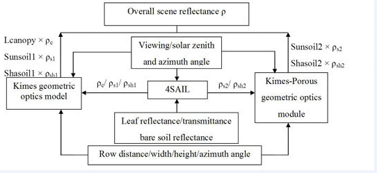
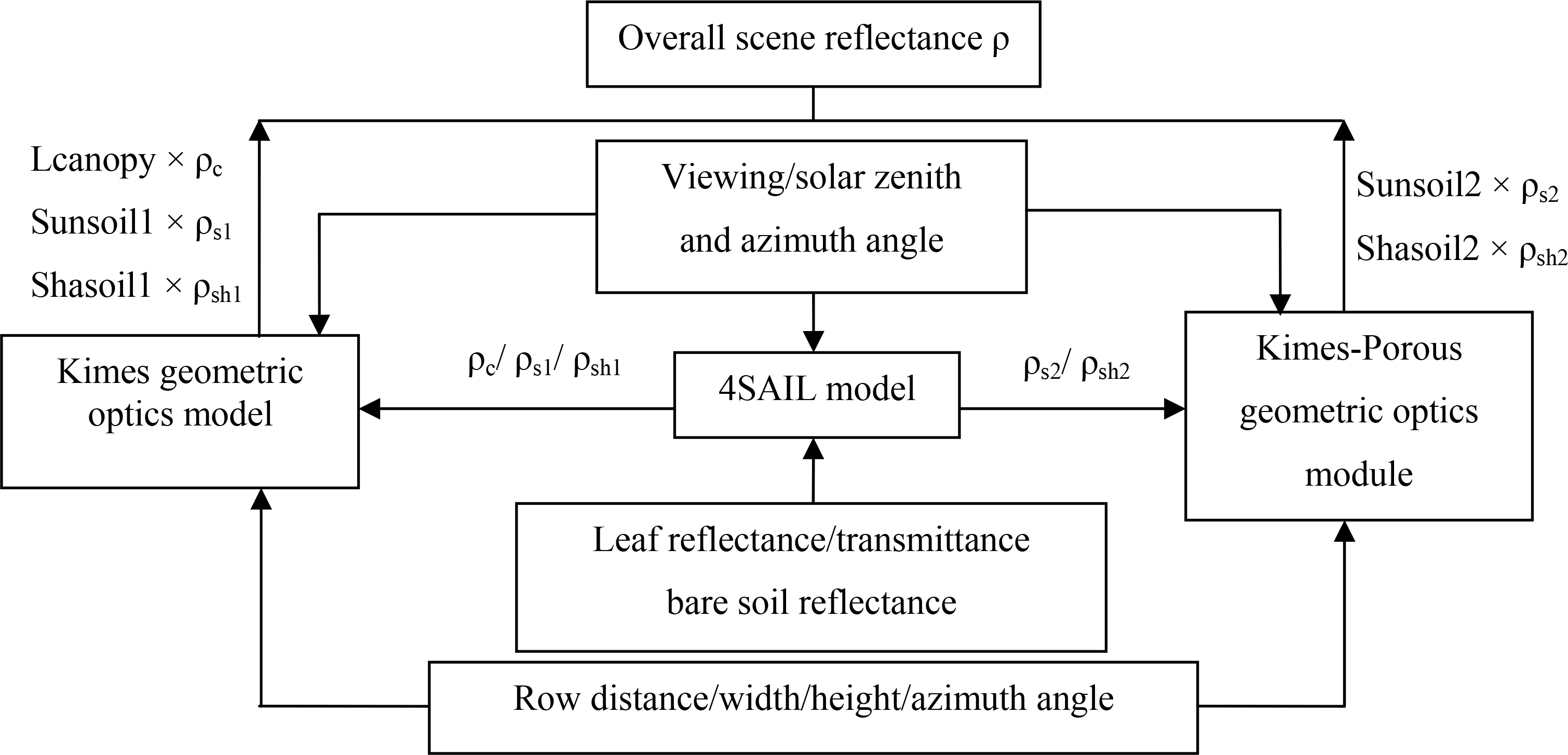
The 4SAIL-RowCrop model was developed by combining the Kimes GO model [12] with the 4SAIL canopy reflectance model [22], in which the 4SAIL model provides RT parameters (reflectance and transmittance) of canopies within rows and the Kimes GO model combines the 4SAIL results into an overall scene reflectance (Figure 1). In order to calculate the overall scene reflectance, the reflectance of each component in the scene was weighted by its fractional area and summed according to Formula (1):
2.2. Modeling Algorithm
The canopy of the row crop was modeled as a porous hedgerow with a rectangular cross-section configuration, similar to the scene reflectance in the GeoSail model [26]. Scene reflectance was determined by calculating an area-weighted average of three landscape components (canopy, sunlit background and shadowed background) in an individual scene of periodic vegetation canopy along rows.
2.2.1. Algorithm of the RT Simulation Module
The 4SAIL model was derived from the four-stream differential equations [22] to avoid the problems associated with mathematical inaccuracies by using a safer and more robust analytical solution than the SAILH model [27,28]. The output from the 4SAIL model integrated sunlit and shaded vegetation, combining these two components from the Kimes model into a single canopy component. The bidirectional reflectance (ρc) of the canopy component was calculated by the 4SAIL model as follows:
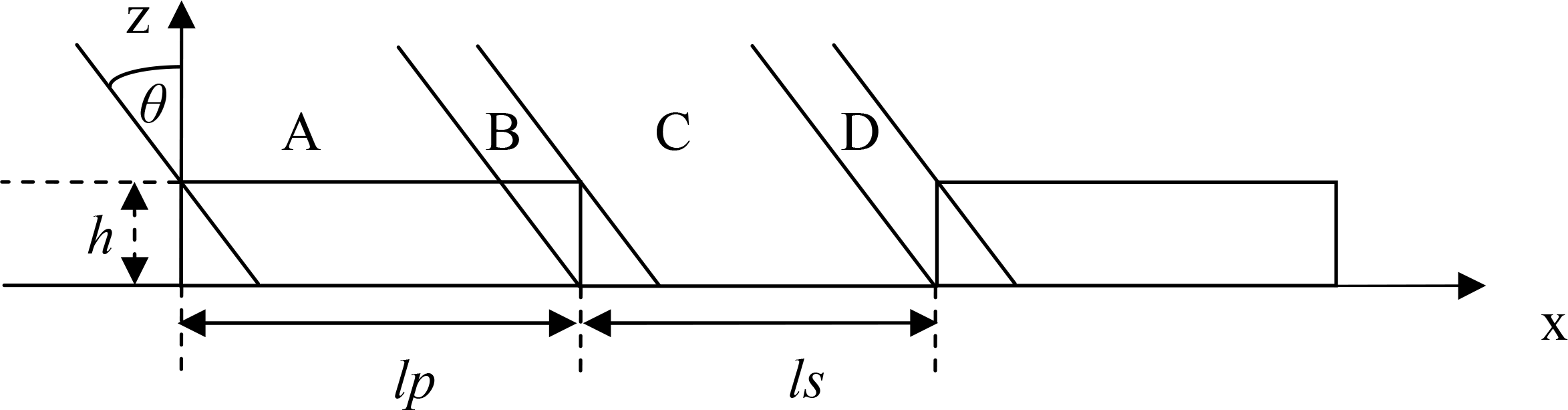
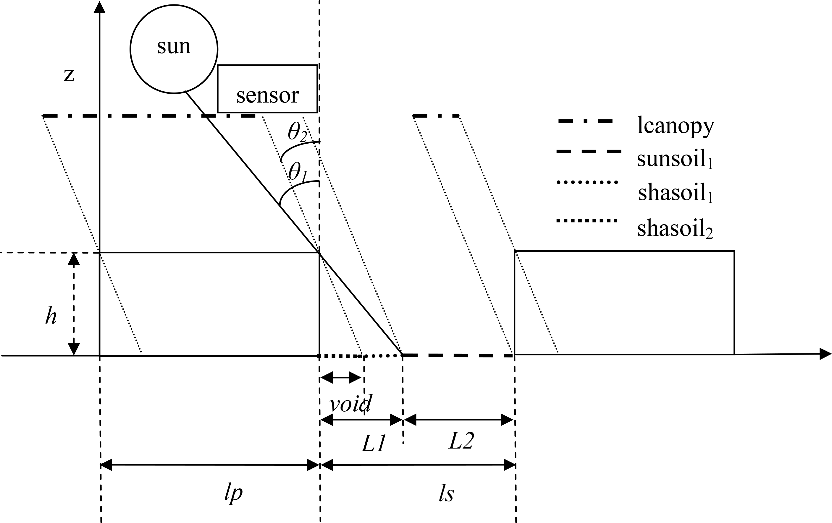
According to the position of the x-axis viewing direction or solar direction cast point, an individual scene of row period was divided into four parts: A, B, C, D (Figure 2). For the continuously homogenous canopy, the average crown transmittance (gap probability) of the direct light in the viewing direction or solar direction was given by:
According to Equations (9) and (10), the average gap probabilities of the four parts (A, B, C, D) were calculated as follows:
2.2.2. Geometric Structure Description of Rice and Wheat Canopy
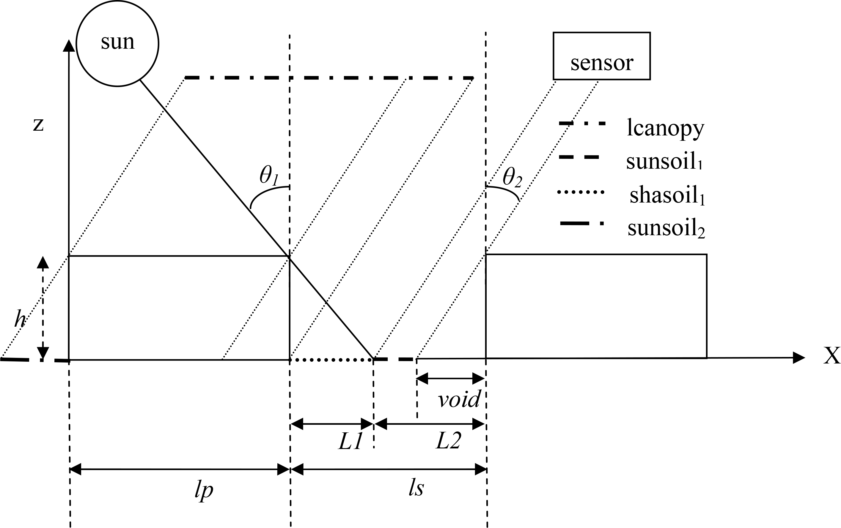
In the 4SAIL-RowCrop model, the shape of the rice and wheat canopy was modeled as a porous hedgerow with a rectangular cross-section configuration, and the row geometry and coordinate system of a cross-row section are shown (Figure 3). The symbols h, lp, ls and ld refer to row height, row width, visible soil strip length between rows and the row distance, respectively.
The solar zenith and azimuth angles and the viewing zenith and azimuth angles were defined as θs and ψs and θv and ψv, respectively. The mean leaf inclination angle was defined as ALA. ψrow represents the row azimuth angle (in the north-south orientation). The azimuth angle was fixed at 0° in the north direction and increased from north to south clockwise from 0° to 360°. The solar-row azimuth and viewing-row azimuth angles were defined as βs and βv, respectively. The solar and viewing directions projected in the plane perpendicular to the rows were represented by their inclination angles θ1 (solar row angle) and θ2 (sensor row angle), respectively. The following relationships applied:
The real leaf area index (LAI) of the row crop was defined as LAIrow, and the mean LAI of the row crop in the field was defined as LAImean. Their relationship was described as:
The relative horizontal projected lengths of the row height on the ground in the Sun direction and in the view direction were defined as L1 and void, respectively, and calculated as follows:
Parameters sunsoil1, shasoil1, sunsoil2 and shasoil2 were defined as the relative projected horizontal length (with direct view to the sensor) of the s1, s2, sh1 and sh2, respectively. The Lcanopy parameter represents the relative projected horizontal length on the ground of the canopy component in the direct line of sight of a particular view direction. Lcanopy, sunsoil1 and shasoil1 were calculated using the Kimes model. Sunsoil2 and shasoil2 were calculated according to three situations based on the geometric relationship between the RS sensor and the sun, as follows:
- (1)
Both sunsoil2 and shasoil2 were equal to 0 when the viewing zenith and azimuth angles were equal to 0° (nadir direction). The relative average crown transmittances ( ) of the direct light in the solar direction derived from the modified 4SAIL model for sh1 were listed in Table 1.
- (2)
Six scenarios occur (L1 ≤ ls ≤ void; ls <L1 ≤ void; L1 > void ≥ ls; L1 ≥ ls and void < ls; void ≤ L1 < ls; L1 ≤ void ≤ ls) when the viewing direction was backwards (the RS sensor was located on the same side as the Sun; Figure 4). The relative average crown transmittances (gap probability, Pθ) are listed in Table 2, in which six scenarios were refined as nine scenarios in the gap probability calculation process. Sunsoil2 and shasoil2 are listed in Table 4.
- (3)
Four scenarios occur (void + L1 ≤ ls; void < ls and L1 + void > ls; void ≥ ls ≥ L1; void ≥ ls and L1 > ls) when the viewing direction was forwards (the RS sensor was located on the opposite side as the Sun; Figure 5). The relative average crown transmittances (gap probability, Pθ) are listed in Table 3, in which four scenarios were refined as five scenarios in the gap probability calculation process. Sunsoil2 and shasoil2 are listed in Table 4.
2.3. Field Data
Two wheat (Triticum aestivum L.) and one rice (Oryza sativa L.) field experiments were conducted to test the performance of the 4SAIL-RowCrop model. These experiments involved different cultivars, sowing dates and nitrogen fertility rates from multiple ecological sites and growth seasons, as shown in Table 5. Spectra for the canopy multi-angle, canopy nadir direction, leaf and soil were measured and synchronized with the measurement of agronomic parameters, such as the LAI and leaf inclination angle of rice and wheat. Two commonly used vegetation indices, the normalized vegetation index (NDVI) [30] and the soil-adjusted vegetation index (SAVI) [31], were also calculated to evaluate the performance of the 4SAIL-RowCrop model (Table 6). The data from rice and wheat experiments in 2012 were used for simulating rice and wheat canopy bidirectional reflectance. The data from rice and wheat experiments in 2004–2005 and rice experiments in 2012 were used for simulating nadir canopy spectral reflectance under different cultivation conditions.
A FieldSpec 3 spectrometer was used to measure the canopy spectra of rice, wheat and soil. This instrument has a spectral range of 350–2500 nm and a sampling interval of 1.4 nm with a spectral resolution of 3 nm between 350 and 1000 nm, and a sampling interval of 2 nm with a spectral resolution of 10 nm between 1000 and 2500 nm. For in situ measurements of canopy reflectance spectra, the sensor was attached to a rod and placed at nadir 2.25 m above the rice canopy, resulting in a view area diameter of approximately 1.0 m, which covered approximately four rows in the cross-row section. The footprint area was an ellipse when the viewing direction was away from the nadir direction. During sunny conditions, all canopy spectral measurements were performed between 10:00 and 14:00 (Beijing local time; solar zenith angle less than 45°). Canopy multi-angle spectra were measured in the principal plane direction with a viewing zenith angle in the range of −60° to 60° and were recorded with an interval angle of 30° for wheat and 10° for rice. Six repeats were performed for each interval angle and five repeats for each plot. Spectra reflectance was acquired for the canopy nadir direction at the same sampling site of the nadir spectra measurement; soil and leaf were measured as described in ASD, and agronomic parameters were determined as described by Li-Cor [32]. Sampling times are shown in Table 3.
Squared correlation coefficients for model validation (R2_VAL), root mean square error (RMSE) and normalized root mean square error (NRMSE, %) were used to calculate the fitness between the estimated and observed values [19] and to evaluate the overall performance of model. In general, all data calculations were implemented with IDL 8.0.
3. Results
3.1. Model Input Parameters
The input parameters of the 4SAIL-RowCrop model and 4SAIL model are listed in Table 7. The solar zenith and solar azimuth angles could be calculated from the latitude, longitude and time of the study area, and the viewing zenith and viewing azimuth angles were obtained from the measurement of canopy spectra. The shade and non-shade ratio of the measured data was taken as a proportion of sky scattered light, and the ratio of direct to total radiation was equal to one minus the proportion of scattered light as measured by an ASD FieldSpec3 2500 spectrometer instrument (Analytical Spectral Devices, Boulder, CO, USA) fitted with a gray reference board. LAI, average leaf inclination angle and the azimuth angle of the ridge were also calculated. Values for line width, ridge spacing and plant height were determined by field measurement, as was soil reflectance. Leaf reflectance and transmittance were calculated using the PROSPECT model [33–37] or measured in the field.
3.2. Rice and Wheat Canopy Bidirectional Reflectance Simulation Analysis
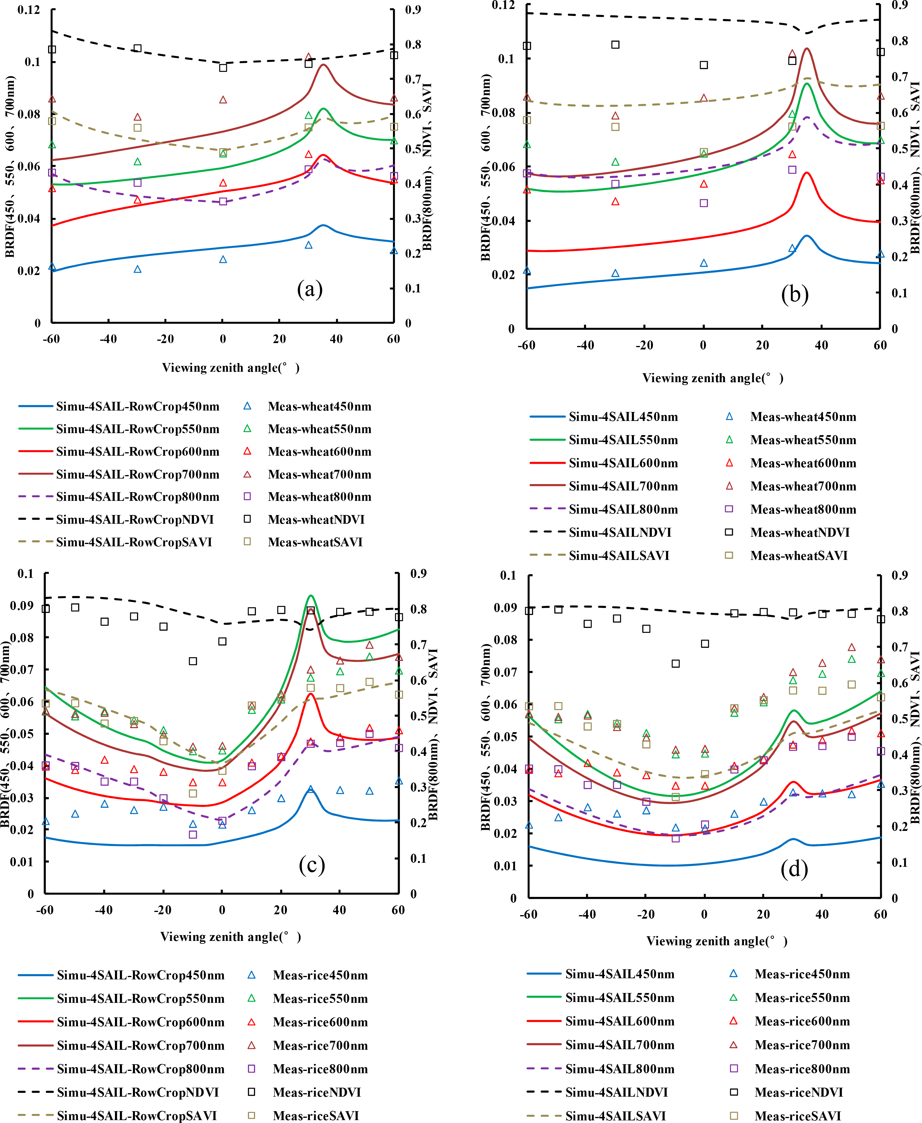
The principal plane (PP) simulated results by the 4SAIL-RowCrop model, red (600 nm, R), blue (450 nm, B), green (550 nm, G), red edge (700 nm, R-edge), NIR (800 nm, Nir), with NDVI and SAVI as examples, were compared with the measured rice and wheat bidirectional reflectance data. The canopy structural parameters, sun/viewing geometrical parameters and optical parameters are listed in Tables 8 and 9, respectively. The visible bands (blue, green, red), red edge bands and NIR bands are important variables for characterizing leaf photosynthesis, the biochemical constituents (e.g., chlorophyll and nitrogen contents) and the biomass and leaf area index of crops, respectively. The NDVI (normalized difference vegetation index) is an important vegetation index, extensively used to indicate vegetation status. To account for changes in the soil optical properties, soil-adjusted indices minimizing the background influence have been developed. The leading index in such improvement is the SAVI (soil-adjusted vegetation index).
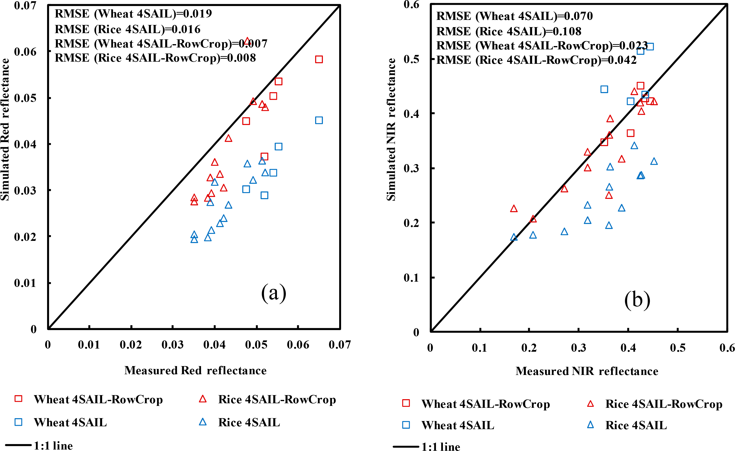
The BRF reflectance of rice and wheat simulated by the 4SAIL-RowCrop model and the 4SAIL model both shared a similar trend and curve shape with the measured reflectance (Figure 6). For wheat, values of the B, G, R and R-edge reflectance decreased with increasing observation zenith angles in the forward direction and in the backward direction, reaching the peak value at the hotspot. However, the values of Nir reflectance, NDVI and SAVI increased with increasing observation zenith angles in both the forward and backward scattering directions and reached minimum values near the nadir direction (zenith angle of 0°; Figure 6a). The 4SAIL-RowCrop model simulated values were slightly higher and lower than the measured values in the B band and G/R-edge bands, respectively. However, the 4SAIL-RowCrop model simulated values were consistent with the measured values of the R/Nir and NDVI/SAVI bands (Figure 6a), and the 4SAIL-RowCrop model simulated values were more close to the measured Nir band reflectance values than the R band reflectance values of wheat canopies. The 4SAIL model simulated values were higher and lower than the measured values in the NIR band and visible/R-edge bands (Figure 7). On the whole, the simulated values were in good agreement with measured values (Table 10).
For rice, the values of G, R and R-edge reflectance increased with increasing viewing zenith angle in the forward and backward directions, whereas B reflectance reached its peak −40° and then decreased in the forward direction. In contrast, Nir reflectance, NDVI and SAVI increased with increasing observation zenith angles in the forward direction (although these values were low at a viewing zenith angle of −10°) and increased in the backward direction up to the peak value at the hotspot. Hotspot reflectance could not be accurately measured by the sensor, due to self-shading and the large field of view of 25°, as previously described [18,19]. The 4SAIL-RowCrop model simulated values were slightly lower than the measured values in the visible and R-edge bands and comparable for the Nir bands and SAVI, and it is clear that the 4SAIL-RowCrop model simulated values were closer to the measured Nir band reflectance values than the R band reflectance values of rice canopies. The 4SAIL model simulated values were lower than the measured values in the NIR band and visible/R-edge bands (Figure 7). This may be caused by the underlying surface specular reflection of the thin layer of water that was included to increase reflectance in the forward direction and decrease reflectance in the backward direction of the visible wavelengths. The overall reflectance values of the bands in the forward direction were lower than those in the backward direction for both wheat and rice (Figure 6a, Figure 6b). The spectra data analysis of rice and wheat indicated that the 4SAIL-RowCrop model performed better than the 4SAIL model.
3.3. Canopy Nadir Spectral Reflectance during Different Growth Stages
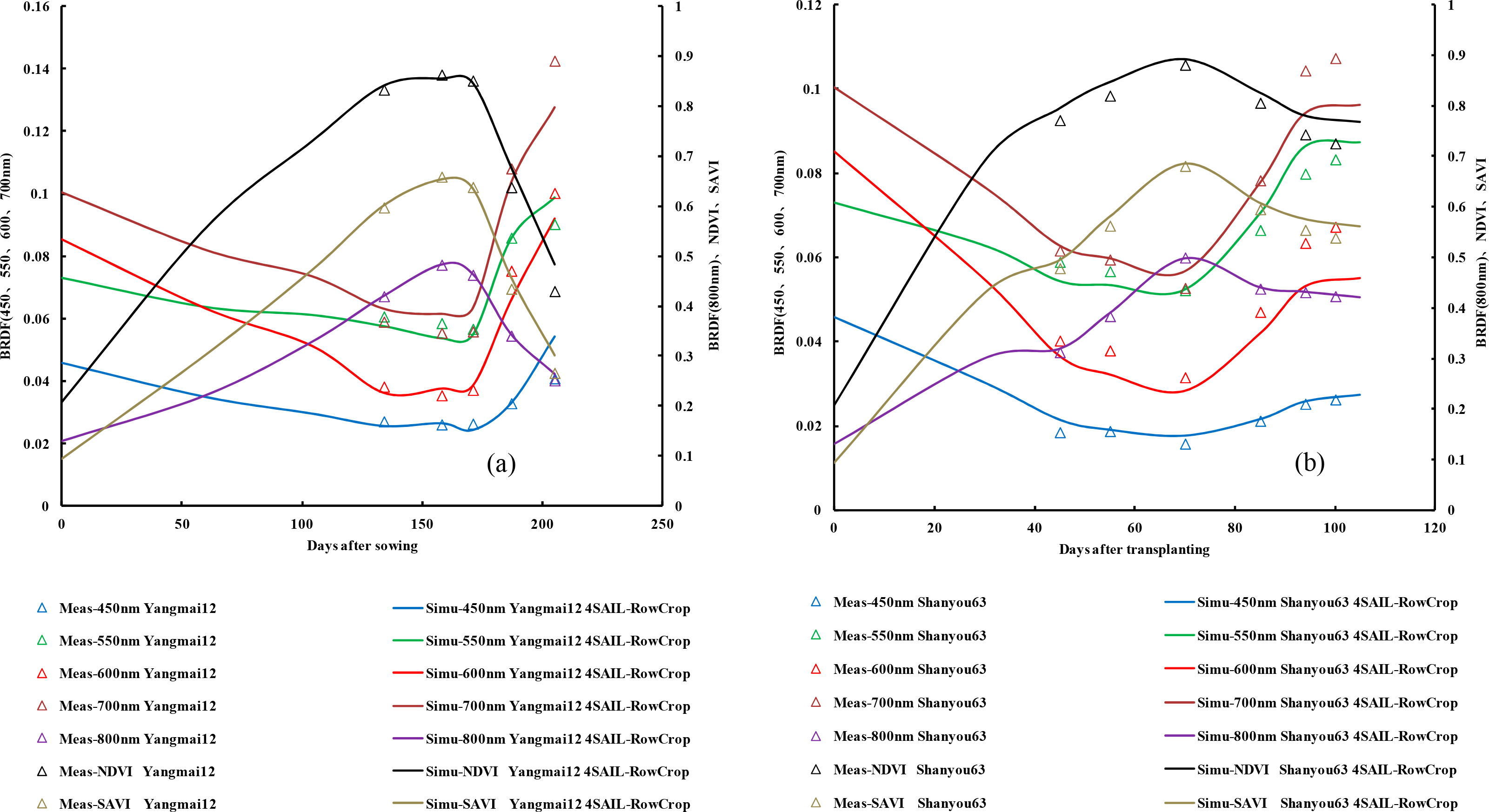
Simulated nadir spectral reflectance and VI values of the 4SAIL-RowCrop model were compared to field measured values during different growth stages. Model parameters were assigned using average values from the validation dataset, and 12:00 noon local time served as the simulation time in the different growth stages. The results showed that the simulated spectral values of the 4SAIL-RowCrop model were highly consistent with measured values during different growth stages in both rice and wheat. Changes in growth patterns under different planting treatments were highly similar irrespective of the different cultivars, nitrogen fertility rates and planting densities. The general trend showed an initial decrease in the R and R-edge bands from the tillering stage to the booting stage and a subsequent increase from the heading stage to the maturity stage. The reflectance of the Nir band exhibited the opposite trend, with values peaking between the booting and heading stages (Yangmai 12 and Shanyou 63 as examples; Figure 8).
Differences between the simulated and measured values for different growth stages were quantitatively compared using the validation dataset. The results showed that the squared correlation coefficient of simulated and measured values for rice and wheat were both above 0.93 (Table 11) over the whole growth circle. In the early growth stages (in which the canopy was not fully covered), the 4SAIL-RowCrop model simulation values gave root mean square error (RMSE) and normalized root mean square error (NRMSE) values of 0.0089 and 6.11%, respectively, whereas in the late growth stage (the canopy was fully covered), the RMSE and NRMSE were 0.0160 and 8.61%, respectively.
For wheat canopies, the Nir band was the most accurately simulated, with RMSE and NRMSE values of 0.0057 and 2.23%, respectively. The B band gave the poorest simulation score, with RMSE and NRMSE values of 0.0061 and 15.34%, respectively. For rice canopies, the best simulation was also the Nir band, with RMSE and NRMSE values of 0.0038 and 1.06%, respectively, while the R band gave the poorest simulation scores (RMSE and NRMSE of 0.0074 and 13.53%, respectively). Overall, these results indicate that the 4SAIL-RowCrop model is capable of accurately modeling the nadir spectral reflectance of rice and wheat during different growth stages.
3.4. Canopy Nadir Spectral Reflectance under Different Cultivation Conditions
The simulated nadir spectra of 4SAIL-RowCrop model for different cultivars (Figure 9a,b), cultivation densities (Figure 9c,d) and nitrogen fertility rates (Figure 9e,f) were compared with field data using the jointing stage dataset for wheat and the filling stage dataset for rice (Table 12). The simulated nadir spectra showed the same overall characteristics as the measured spectra irrespective of the cultivation conditions.
For the rice canopy, reflectance in the G, R and Nir bands was higher for cultivar Shanyou 63 than for Wuxiangjing 14 (Figure 9a). There were significant increases in the R-edge and Nir spectra and more subtle changes in the visible bands with increased cultivation densities (Wuxiangjing 14 as an example; Figure 9c). Spectral reflectance decreased in the visible bands, but increased in the R-edge and Nir bands with increasing nitrogen fertility rates (Wuxiangjing 14 as an example; Figure 9e). These spectral characteristics were the same for different rice cultivars (Shanyou 63 and Wuxiangjing 14). For the wheat canopy, the canopy reflectance values of Yangmai 12 were higher in the Nir bands and slightly lower in the visible bands (Figure 9b), and this trend was retained irrespective of cultivation density and nitrogen fertility rate (Ningmai 9 as an example; Figure 9d,f).
The squared correlation coefficients of simulated and observed values were approximately 0.9 for both rice and wheat under a variety of conditions (Table 12), supporting the reliability of the 4SAIL-RowCrop model for simulating the canopy nadir direction spectral reflectance under different cultivation conditions in rice and wheat.
4. Discussion
In this study, a novel row crop GO-RT bidirectional reflectance model (4SAIL-RowCrop) was developed by coupling the 4SAIL and Kimes models. GO models considered the row crops as opaque rectangular solids without simulating the multiple-scattering radiation transfer process within the canopy, which resulted in the bad simulation of the reflectance of NIR bands [19]. The effect of canopy heterogeneity on bidirectional reflectance for the row-planted crops canopies were not appropriately quantified by RT models, because of less consideration for the geometrical structure parameters [24]. Thus, combining the GO model and the RT model may be a good approach to better simulate the bidirectional reflectance of the row-planted crops canopies despite that a row RT model was developed by Zhao et al. [19] based on the four-stream SAIL model and performed well in winter wheat. Therefore, in this paper, the 4SAIL-RowCrop model was developed by simultaneously taking into consideration row crop geometry and canopy RT processes, which overcame the failings of the previous 4SAIL model in simulating row crop bidirectional reflectance [22] and performed well in both row-planted rice and wheat. However, the 4SAIL-RowCrop model can be further evaluated and compared with the published row model developed by Zhao et al. [19] in future work. Furthermore, the inversion of the 4SAIL-RowCrop model will be a research topic in our future work. Since the 4SAIL-RowCrop model needs over ten input parameters, a priori knowledge of the row-planted rice and wheat should be provided (e.g., some structural parameters: row width, row height) in order to get an improved performance for biophysical parameter mapping. Moreover, when the prior information of input parameters is provided, it is strongly recommended to implement algorithms from increasing the dimensionality of the feature space to the use of neighborhood information [38], mitigating the ill-posed inverse problem and, thus, leading to higher estimation accuracies.
The multiple scattering of the inter-dune soil between the rows was also considered in the 4SAIL-RowCrop model in order to improve the accuracy of the reflectance values [18]. However, the simulated reflectance values generated by the model were lower than values measured in the field for R-edge bands, which may be due to the dependence of R-edge reflectance on crop type and nitrogen concentrations [39]. Inaccuracies in the field measurements of the canopy structure parameters and spectral data may also introduce errors. The 4SAIL-RowCrop model performed better with wheat than with rice overall. This is likely due to the surface specular reflection from the thin water layer present under the rice canopies, which increased the visible spectral reflectance of the simulations in the forward direction and lowered this parameter in the backward direction. Therefore, further work is required to quantify the specific impact of the water on the canopy reflectance spectra for rice. When the solar or viewing azimuth angle and the row orientation angle are very close to each other, the soil between rows has a large proportion of contribution to the scene reflectance, which makes the simulated results of 4SAIL-RowCrop model higher than the 4SAIL simulated results. However, this is not the case when there was a large difference between the solar or viewing azimuth angle and the row orientation angle. This is probably due to the use of the LAIrow parameter in the 4SAIL-RowCrop model instead of LAImean, which was used in the 4SAIL model. LAImean is lower than LAIrow, because the within-row crop LAI is the product of row crop mean LAI and row distance divided by row width, which lowers the simulated reflectance in the 4SAIL model. Moreover, the soil between row reflectance had a big influence on the red band, so the 4SAIL-RowCrop model always simulated slightly higher reflectance values than the 4SAIL model. Notably, reflectance in the forward direction was lower than that in the backward direction for all bands. This may be explained by the hotspot effect that occurs in the backward direction of row-planted crops.
The results from different cultivation conditions also indicated that the 4SAIL-RowCrop model performed better for modeling nadir direction reflectance spectra than for modeling bidirectional reflectance spectra. This may be due to the fact that the nadir directional canopy spectra are measured vertically and so are limited by differences in the layers corresponding to leaf nutrient content, structural parameters and environment. Moreover, the contribution made by different layers to the canopy reflectance spectra change with the viewing direction [40]. With both wheat and rice canopies, the nadir directional and bidirectional reflectance spectra were most accurately simulated for the Nir band, with NRMSE values of less than 14.4%. The simulation of bi-directional reflectance in the visible bands was significantly less accurate, and the B band was simulated with the poorest accuracy, with NRMSE values over 15.3%. Improving the accuracy of the simulation of the bidirectional reflectance in the visible bands is a target for future work.
The 4SAIL-RowCrop model performed well during the earlier stages (referring to the tillering stage, jointing stage, up to the booting stage) of growth before crop canopy closure occurred. This suggested that the contributions of sunlit soil and shaded soil to the canopy reflectance spectra in the 4SAIL-RowCrop model were superior to those in the 4SAIL model [22]. However, the wheat and rice crops at the juvenile stage or seedling stage cannot be considered as a hedgerow, so we suggest this new model be used from the tillering stage. Moreover, after canopy closure in rice and wheat (from the heading stage to the maturity stage), the precision of the simulation was somewhat lower, as previously observed by Li et al. [41]. This may be due to the model ignoring the impact of spikes. In the later growth stages of rice and wheat, spikes can last over a month, and both spikes and leaves affect canopy reflectance characteristics. Furthermore, the spikes of rice and wheat are higher in the row direction at the top of the canopies; therefore, spikes may affect leaf layer and soil layer radiation [17]. Spikes may cover leaves during the late growth stages after heading, and the radiation measured by the sensor would be dependent on the contributions from soil, leaves and spikes; this should be taken into consideration in future models.
In addition, soil was assumed to behave in a Lambertian manner, and soil spectra were considered constant throughout the growth circle in the 4SAIL-RowCrop model. This ignores the directional simulated reflectance characteristics of soil [22] and may introduce errors in the overall canopy reflectance simulation. In future models, the bidirectional reflectance of soil should be incorporated. Another assumption was that leaves were randomly distributed, and this ignores the effects of clumping. Parameterization of clumping effects along the row direction should also be included in future models to more accurately simulate the spatial distribution of leaves in the canopy.
5. Conclusions
The paper presents the development and implementation of a novel and efficient canopy reflectance model (4SAIL-RowCrop) capable of simulating the bidirectional reflectance of row-planted rice and wheat canopies. The bidirectional reflectance and nadir reflectance simulated by the 4SAIL-RowCrop model were in good agreement with field measurements, with squared correlation coefficients of 0.69 and 0.98, root mean square errors of 0.013 and 0.009 and normalized root mean squared errors of 15.8% and 12.4%, respectively. These results demonstrated the ability of the 4SAIL-RowCrop model to accurately simulate the bidirectional reflectance and nadir reflectance of row-planted rice and wheat canopies.
The 4SAIL-RowCrop model performed better for modeling nadir reflectance than for modeling bidirectional reflectance. Moreover, the 4SAIL-RowCrop model performed better for wheat canopies than for rice canopies. Furthermore, the wheat and rice crops at the juvenile stage or seedling stage cannot be considered as a hedgerow. The precision of the simulation was slightly lower after canopy closure in rice and wheat (from the heading stage to the maturity stage). Therefore, we suggest the 4SAIL-RowCrop model be used from the tillering stage to the heading stage.
This research is expected to use remotely sensed data for assessing the living status of the row-planted crops (rice and wheat) and predicting the yield of row-planted crops. The study will also contribute to the efforts of improved performance for biophysical parameter mapping. This promising model requires further testing under a wider range of conditions and will benefit from refinements that allow its use in multiple crop production systems.
Acknowledgments
This work was supported by grants from the National High Technology Research and Development Program of China (863 Program, 2013AA102301), the National Natural Science Foundation of China (31371535), the Special Fund for Agro-scientific Research in the Public Interest (201303109), the Science and Technology Support Program of China (2013BAD20B05), Jiangsu Science and Technology Support Program (BE2011351 and BE2012302), Jiangsu Collaborative Innovation Center for Modern Crop Production and the Priority Academic Program Development of Jiangsu Higher Education Institutions (PAPD), China. The extensive English revisions of the manuscript checked by Tao Cheng are deeply appreciated.
Author Contributions
Kai Zhou developed the model, collected field reflectance data, performed the data analysis, results interpretation, manuscript writing and coordinated the revision activities. Yongjiu Guo and Yanan Geng assisted with the process of field reflectance data collection and results interpretation. Yan Zhu and Weixing Cao assisted with developing the research design, results interpretation and manuscript writing. Yongchao Tian proposed the research design and manuscript revision.
Conflicts of Interest
The authors declare no conflict of interest.
References
- Suits, G.H. Extension of a uniform canopy reflectance model to include row effects. Remote Sens. Environ 1983, 13, 113–129. [Google Scholar]
- Annandale, J.G.; Jovanovic, N.Z.; Campbell, G.S.; Du Sautoy, N.; Lobit, P. Two dimensional solar radiation interception model for hedgerow fruit trees. Agric. For. Meteorol 2004, 121, 207–225. [Google Scholar]
- Bégué, A.; Roujean, J.L.; Hanan, N.P.; Prince, S.D.; Thawley, M.; Huete, A. Shortwave radiation budget of Sahelian vegetation 1. Techniques of measurement and results during HAPEX-Sahel. Agric. For. Meteorol 1994, 79, 79–96. [Google Scholar]
- Ganis, A. Radiation transfer estimate in a row canopy: A simple procedure. Agric. For. Meteorol 1997, 88, 67–76. [Google Scholar]
- Goel, N.S.; Grier, T. Estimation of canopy parameters for inhomogeneous vegetation canopies from reflectance data I. Two-dimensional row canopy. Int. J. Remote. Sens 1986, 7, 665–681. [Google Scholar]
- Nilson, T.; Kuusk, A. A reflectance model for the homogeneous plant canopy and its inversion. Remote Sens. Environ 1989, 27, 157–167. [Google Scholar]
- Suits, G.H. The calculation of the directional reflectance of a vegetative canopy. Remote Sens. Environ 1972, 2, 117–125. [Google Scholar]
- Schaepman-Strub, G.; Schaepman, M.E.; Painter, T.H.; Dangel, S.; Martonchik, J.V. Reflectance quantities in optical remote sensing-definitions and case studies. Remote Sens. Environ 2006, 103, 27–42. [Google Scholar]
- Verhoef, W.; Bunnik, N.J.J. The Spectral Directional Reflectance of Row Crops; Netherlands Interdepartmental Working Group on the Application of Remote Sensing: Delft, The Netherlands, 1976; p. 135. [Google Scholar]
- Verhoef, W. Light scattering by leaf layers with application to canopy reflectance modeling: The SAIL model. Remote Sens. Environ 1984, 6, 125–184. [Google Scholar]
- Jackson, R.D.; Reginato, R.J.; Pinter, P.J., Jr.; Idso, S.B. Plant canopy information extraction from composite scene reflectance of row crops. Appl. Opt 1979, 18, 3775–3782. [Google Scholar]
- Kimes, D.S. Remote sensing of row crop structure and component temperatures using directional radiometric temperatures and inversion techniques. Remote Sens. Environ 1983, 13, 33–55. [Google Scholar]
- Verbrugghe, M.; Cierniewski, J. Effects of sun and view geometries on cotton bidirectional reflectance test of a geometrical model. Remote Sens. Environ 1995, 54, 189–197. [Google Scholar]
- Chen, L.F.; Liu, Q.H.; Fan, W.J.; Li, X.W.; Xiao, Q.; Yan, G.J.; Tian, G.L. A bi-directional gap model for simulating the directional thermal radiance of row crops. Sci. China Ser. D-Earth Sci. 2002, 45, 1087–1098. [Google Scholar]
- Yan, G.J.; Jiang, L.M.; Wang, J.D.; Chen, L.F.; Li, X.W. Thermal bidirectional gap probability model for row crop canopies and validation. Sci. China Ser. D-Earth Sci 2003, 46, 1241–1249. [Google Scholar]
- Yu, T.; Gu, X.F.; Tian, G.L.; Legrand, M.; Baret, F.; Hanocq, J.F.; Bosseno, R.; Zhang, Y. Modeling directional brightness temperature over amaize canopy in row structure. IEEE Trans. Geosci. Remote Sens 2004, 42, 2290–2304. [Google Scholar]
- Du, Y.; Liu, Q.; Chen, L.; Liu, Q.; Yu, T. Modeling directional brightness temperature of the winter wheat canopy at the ear stage. IEEE Trans. Geosci. Remote Sens. 2007, 45, 3721–3739. [Google Scholar]
- Yan, B.Y.; Xu, X.R.; Fan, W.J. A unified canopy bidirectional reflectance (BRDF) model for row crops. Sci. China Ser. D-Earth Sci 2012, 55, 824–836. [Google Scholar]
- Zhao, F.; Gu, X.F.; Verhoef, W.; Wang, Q.; Yu, T.; Liu, Q.; Huang, H.G.; Qin, W.H.; Chen, L.F.; Zhao, H.J.; et al. A spectral directional reflectance model of row crops. Remote Sens. Environ 2010, 114, 265–285. [Google Scholar]
- Yao, Y.J.; Liu, Q.H..; Liu, Q.; Li, X.W. LAI retrieval and uncertainty evaluations for typical row-planted crops at different growth stages. Remote Sens. Environ 2008, 112, 94–106. [Google Scholar]
- Li, X.W.; Wang, J.D. Plant Phot on Remote Sensing Model and Parameterizing of Plant Structure, 1st ed.; Science Press: Beijing, China, 1995; pp. 118–119. (In Chinese) [Google Scholar]
- Verhoef, W.; Jia, L.; Xiao, Q.; Su, Z. Unified optical-thermal four-stream radiative transfer theory for homogeneous vegetation canopies. IEEE Trans. Geosci. Remote Sens 2007, 45, 1808–1822. [Google Scholar]
- Li, X.W.; Strahler, A.H. Geometric-optical bidirectional reflectance modeling of a conifer forest canopy. IEEE Trans. Geosci. Remote Sens 1985, 24, 906–919. [Google Scholar]
- Atzberger, C. Development of an invertible forest reflectance model: The INFOR-Model. A decade of trans-European remote sensing cooperation. Proceedings of the 20th EARSeL Symposium, Dresden, Germany, 14–16 June 2000; pp. 39–44.
- Atzberger, C.; Schlerf, M. Inversion of a forest reflectance model to estimate structural canopy variables from hyperspectral remote sensing data. Remote Sens. Environ 2006, 100, 281–294. [Google Scholar]
- Huemmrich, K.F. The GeoSAIL model: A simple addition to the SAIL model to describe discontinuous canopy reflectance. Remote Sens. Environ 2001, 75, 423–431. [Google Scholar]
- Verhoef, W. Earth observation modeling based on layer scattering matrices. Remote Sens. Environ 1985, 17, 165–178. [Google Scholar]
- Verhoef, W. Theory of Radiative Transfer Models Applied in Optical Remote Sensing of Vegetation Canopies., Ph.D. Dissertation. Wageningen Agricultural University, Wageningen, The Netherlands, 1998.
- Jacquemoud, S.; Verhoef, W.; Baret, F.; Bacour, C.; Zarco-Tejada, P.J.; Asner, G.P.; Francois, C.; Ustin, S.L. PROSPECT plus SAIL models: A review of use for vegetation characterization. Remote Sens. Environ 2009, 113, S56–S66. [Google Scholar]
- Rouse, J.W.; Haas, R.H.; Schell, J.A.; Deering, D.W.; Harlan, J.C. Monitoring the Vernal Advancement of Retrogradation of Natural Vegetation; Final Report; NASA/GSFC: Greenbelt, MD, USA, 1974; p. 137. [Google Scholar]
- Huete, A. A soil-adjusted vegetation index (SAVI). Remote Sens. Environ 1988, 25, 295–309. [Google Scholar]
- Li-Cor. LAI-2000 Plant Canopy Analyzer Operating Manual; Li-Cor, Inc.: Lincoln, NE, USA, 1991. [Google Scholar]
- Jacquemoud, S.; Baret, F. PROSPECT: A model of leaf optical properties spectra. Remote Sens. Environ 1990, 34, 75–91. [Google Scholar]
- Jacquemoud, S.; Ustin, S.L.; Verdebout, J.; Schmuck, G.; Andreoli, G.; Hosgood, B. Estimating leaf biochemistry using the PROSPECT leaf optical properties model. Remote Sens. Environ 1996, 56, 194–202. [Google Scholar]
- Baret, F.; Fourty, T. Estimation of leaf water content and specific leaf weight from reflectance and transmittance measurements. Agronomie 1997, 17, 455–464. [Google Scholar]
- Féret, J.B.; Francois, C.; Asner, G.P.; Gitelson, A.A; Martin, R.E.; Bidel, L.P.R.; Ustin, S.L.; Le Maire, G.; Jacquemoud, S. PROSPECT-4 and 5: Advances in the leaf optical properties model separating photosynthetic pigments. Remote Sens. Environ 2008, 112, 3030–3043. [Google Scholar]
- Bousquet, L.; Lachérade, S.; Jacquemoud, S.; Moya, I. Leaf BRDF measurement and model for specular and diffuse component differentiation. Remote Sens. Environ 2005, 98, 201–211. [Google Scholar]
- Atzberger, C.; Richter, K. Spatially constrained inversion of radiative transfer models for improved LAI mapping from future Sentinel-2 imagery. Remote Sens. Environ 2012, 120, 208–218. [Google Scholar]
- Zhu, Y.; Zhou, D.; Yao, X.; Tian, Y.; Cao, W. Quantitative relationships of leaf nitrogen status to canopy spectral reflectance in rice. AusT. J. Agric. Res. 2007, 58, 1077–1085. [Google Scholar]
- Wang, J.; Zhao, C.; Huang, W. The Foundation of Agricultural Quantitative Remote Sensing Applications, 1st ed.; Science Press: Beijing, China, 2008; pp. 178–179. (In Chinese) [Google Scholar]
- Li, Y.M.; Wang, R.C.; Wang, X.Z.; Shen, Z.Q.; Shen, G.R. Simulation of bi-directional reflectance on rice canopy and its inversion. Chin. J. Rice Sci. 2002, 16, 291–294. (In Chinese). [Google Scholar]


| Situation | Shasoil1 | |
|---|---|---|
| 0 < L1 ≤ lp and 0< L1≤ ls | L1 | |
| lp < L1 < ls | L1 | |
| Lp ≤ ls < L1 < lp + ls | ls | |
| Lp < ls < lp + ls < L1 | ls | τss |
| Ls < L1 < lp | ls | |
| Ls < lp < L1 < lp + ls | ls |
Notes: kss is −ln(τss)/h. θs is the solar zenith angle. τss is the average crown transmittance (gap probability) of the direct light in the solar direction from the 4SAIL model.
| Situation | ||||
|---|---|---|---|---|
| L1 ≤ ls ≤ void | Null | τoo | ||
| Ls < L1 ≤ void | Null | Null | ||
| L1 > void ≥ ls | Null | Null | ||
| Void < ls < L1 | Null | τss | ||
| Void ≤ lp ≤ L1 < ls | Null | τss | ||
| Lp < void < L1 ≤ ls | Null | |||
| L1 < void < ls and void < lp + L1 | Null | |||
| L1 < lp + L1 < void < ls | Null | τoo | ||
| L1 < void < ls and void < lp | Null |
Notes: θs and θo are the solar zenith angle and viewing zenith angle. τss and τoo are the average crown transmittance (gap probability) of the direct light in the solar direction and viewing direction from the 4SAIL model. kss is −ln(τss)/h, and koo is −ln(τoo)/h respectively. is the modified average crown transmittance (gap probability) of the direct light in the viewing direction based on the 4SAIL model for s2. is the average crown transmittance (gap probability) of the direct light in the sun direction modified from the 4SAIL model for sh1. and are the modified average crown transmittance (gap probability) of the direct light in the viewing direction and solar direction based on the 4SAIL model for sh2. Null denotes that this parameter is null in specific situations.
| Situation | ||||
|---|---|---|---|---|
| Void + L1 ≤ ls and L1 < lp | Null | Null | ||
| Lp < L1 ≤ ls-void | Null | Null | ||
| Void < ls < L1 + void | ||||
| Void ≥ ls ≥ L1 | τoo | Null | ||
| Void ≥ ls and L1 > ls | Null | Null |
Notes: θs and θo are the solar zenith angle and viewing zenith angle. τss and τoo are the average crown transmittance (gap probability) of the direct light in the solar direction and viewing direction from the 4SAIL model. kss is −ln(τss)/h, and koo is −ln(τoo)/h respectively. is the modified average crown transmittance (gap probability) of the direct light in the viewing direction based on the 4SAIL model for s2. is the average crown transmittance (gap probability) of the direct light in the sun direction modified from the 4SAIL model for sh1. and are the modified average crown transmittance (gap probability) of the direct light in the viewing direction and solar direction based on the 4SAIL model for sh2. Null denotes that this parameter is null in specific situations.
| Viewing Direction | Situation | Sunsoil2 | Shasoil2 |
|---|---|---|---|
| Backward | L1 ≤ ls ≤ void | ls-L1 | L1 |
| Backward | Ls < L1 ≤ void | 0 | ls |
| Backward | L1 > void ≥ ls | 0 | ls |
| Backward | L1 ≥ ls and void < ls | 0 | void |
| Backward | void ≤ L1 < ls | 0 | void |
| Backward | L1 ≤ void ≤ ls | void-L1 | L1 |
| Forward | void + L1 ≤ ls | void | 0 |
| Forward | void < ls < L1 + void | ls-L1 | L1 + void-ls |
| Forward | void ≥ ls ≥ L1 | ls-L1 | L1 |
| Forward | void ≥ ls and L1 > ls | 0 | ls |
| Year | Crop | Site Location | Cultivar | Nitrogen Rate | Planting Density | Sampling Date | Planting Data |
|---|---|---|---|---|---|---|---|
| (kg·hm−2) | |||||||
| 2004–2005 | wheat | Nanjing 118°78′E 32°04′N | Ningmai 9 | 0, 75, 150, 225 | 150 plants/m2 | 3/19, 4/13, 4/26 | 11/5 |
| Yangmai 12 | 5/3, 5/6, 5/12 | ||||||
| Yumai 34 | 5/20, 5/24, 6/1 | ||||||
| 2011–2012 | wheat | Rugao 120°45′E 32°16′N | Yangmai 16 | 225 | 75, 150 plants/m2 | 3/12 *, 3/26 | 10/15 |
| 225, 300 plants/m2 | 4/7, 4/15 | 10/30 | |||||
| 375, 450 plants/m2 | 11/14 | ||||||
| 2012 | rice | Rugao 120°45′E 32°16′N | Wuxiangjing14 | 0, 150, 250, 350 | 13.3 plants/m2 | 7/22, 8/6, 8/19 | 6/22 |
| Shanyou63 | 22.2 plants/m2 | 8/31 *, 9/15, 9/24 |
Note:*denotes the sampling date of bidirectional spectra.
| VI | Algorithm | Reference |
|---|---|---|
| NDVI (λ1,λ2) | (RNir − RRed) / (RNir + RRed) | Rouse et al. (1974) [30] |
| SAVI | 1.5×(RNir − RRed) / (RNir + RRed + 0.5) | Huete (1988) [31] |
Notes: RNir denotes the near-infrared band reflectance, RRed denotes the red band reflectance.
| Input Parameters | 4SAIL-RowCrop Model | 4SAIL Model |
|---|---|---|
| Geometry and illumination parameters | Solar zenith angle | Solar zenith angle |
| Solar azimuth angle | Solar azimuth angle | |
| Viewing zenith angle | Viewing zenith angle | |
| Viewing azimuth angle | Viewing azimuth angle | |
| Ratio of direct radiation to total radiation | Ratio of direct radiation to total radiation | |
| Canopy geometry parameters | Average leaf area index | Average leaf area index |
| Row width | ||
| Average leaf inclination angle | Average leaf inclination angle | |
| Ridge spacing | ||
| Plant height | ||
| Azimuth angle of ridge | ||
| Optical parameters | Leaf reflectance/transmittance | Leaf reflectance/transmittance |
| Soil reflectance | Soil reflectance | |
| Date | lp * | ls * | h * | LAImean | θs | ψs | ψv | ψrow * | ALA |
|---|---|---|---|---|---|---|---|---|---|
| 12 March 2012 | 0.13 | 0.12 | 0.21 | 2.0 | 35.7° | 185.9° | 180° | 175° | 40° |
| 30 August 2012 | 0.29 | 0.21 | 0.79 | 2.3 | 28.7° | 140.6° | 140° | 175° | 72° |
Notes:*indicates parameters unique to the 4SAIL-RowCrop model; lp *, ls *, h * and ψrow * denote the row width, visible soil strip length between rows, row height and row azimuth angle in north-south orientation, respectively.
| Date | Band | ρleaf | τleaf | ρsoil | Sλ/Qλ |
|---|---|---|---|---|---|
| 12 March 2012 | Red | 0.065 | 0.062 | 0.085 | 0.91 |
| NIR | 0.482 | 0.474 | 0.131 | 0.91 | |
| Blue | 0.045 | 0.041 | 0.046 | 0.91 | |
| Green | 0.111 | 0.113 | 0.073 | 0.91 | |
| Red edge | 0.119 | 0.129 | 0.101 | 0.91 | |
| 30 August 2012 | Red | 0.081 | 0.091 | 0.079 | 0.89 |
| NIR | 0.461 | 0.467 | 0.116 | 0.89 | |
| Blue | 0.042 | 0.044 | 0.062 | 0.89 | |
| Green | 0.134 | 0.151 | 0.082 | 0.89 | |
| Red edge | 0.124 | 0.137 | 0.083 | 0.89 | |
Notes: red, NIR, blue, green and red edge bands are 600, 800, 450, 550 and 700 nm, respectively. ρleaf, τleaf, ρsoil and Sλ/Qλ denote leaf reflectance and transmission, soil reflectance and the proportion of the total spectral solar irradiance to the total spectral solar irradiance in a horizontal plane above the plant canopy, respectively.
| Crop Types | Spectra Bands and VIs | (R2_VAL) | RMSE | NRMSE (%) | |||
|---|---|---|---|---|---|---|---|
| 4SAIL-RowCrop | 4SAIL | 4SAIL-RowCrop | 4SAIL | 4SAIL-RowCrop | 4SAIL | ||
| Wheat | Red | 0.5776 | 0.8281 | 0.007 | 0.019 | 13.7 | 35.6 |
| NIR | 0.6889 | 0.2401 | 0.023 | 0.070 | 5.6 | 17.6 | |
| Blue | 0.7396 | 0.8836 | 0.004 | 0.004 | 15.3 | 18.1 | |
| Green | 0.6084 | 0.7225 | 0.008 | 0.010 | 12.4 | 14.2 | |
| Red edge | 0.5329 | 0.7056 | 0.015 | 0.021 | 16.9 | 24.2 | |
| NDVI | 0.6084 | 0.5041 | 0.027 | 0.096 | 3.4 | 12.7 | |
| SAVI | 0.6724 | 0.0676 | 0.024 | 0.099 | 4.2 | 18.6 | |
| Rice | Red | 0.7225 | 0.7396 | 0.008 | 0.016 | 18.5 | 37.4 |
| NIR | 0.7569 | 0.6724 | 0.042 | 0.108 | 14.4 | 29.1 | |
| Blue | 0.5625 | 0.5625 | 0.009 | 0.014 | 32.4 | 50.8 | |
| Green | 0.8281 | 0.7569 | 0.009 | 0.014 | 14.6 | 24.8 | |
| Red edge | 0.8281 | 0.8100 | 0.008 | 0.019 | 14.2 | 31.8 | |
| NDVI | 0.0324 | 0.0004 | 0.052 | 0.052 | 7.3 | 7.6 | |
| SAVI | 0.6561 | 0.6084 | 0.054 | 0.098 | 13.9 | 18.8 | |
Notes: red, NIR, blue, green and red edge bands are 600, 800, 450, 550 and 700 nm, respectively.VI = vegetation index.
| Crop Type | Spectra Band and VI | 4SAIL-RowCrop Model | ||
|---|---|---|---|---|
| (R2_VAL) | RMSE | NRMSE (%) | ||
| Wheat | Red | 0.9900 | 0.0058 | 7.78 |
| NIR | 0.9980 | 0.0057 | 2.23 | |
| Blue | 0.9584 | 0.0061 | 15.34 | |
| Green | 0.9801 | 0.0046 | 6.17 | |
| Red edge | 0.9980 | 0.0084 | 9.79 | |
| NDVI | 0.9980 | 0.0299 | 6.19 | |
| SAVI | 0.9980 | 0.0188 | 6.33 | |
| Rice | Red | 0.9900 | 0.0074 | 13.53 |
| NIR | 0.9980 | 0.0038 | 1.06 | |
| Blue | 0.9351 | 0.0015 | 8.05 | |
| Green | 0.9722 | 0.0042 | 5.99 | |
| Red edge | 0.9940 | 0.0064 | 6.57 | |
| NDVI | 0.9900 | 0.0287 | 3.79 | |
| SAVI | 0.9960 | 0.0172 | 3.18 | |
Notes: red, NIR, blue, green and red edge bands are 600, 800, 450, 550 and 700 nm, respectively.VI = vegetation index.
| Crop Type | Spectra Band and VI | 4SAIL-RowCrop Model | ||
|---|---|---|---|---|
| (R2_VAL) | RMSE | NRMSE (%) | ||
| Wheat | Blue | 0.8446 | 0.0018 | 7.06 |
| Green | 0.9643 | 0.0027 | 4.04 | |
| Red | 0.9584 | 0.0022 | 5.91 | |
| Red edge | 0.9663 | 0.0069 | 11.73 | |
| NIR | 0.9980 | 0.0046 | 1.02 | |
| NDVI | 0.9821 | 0.0086 | 1.05 | |
| SAVI | 0.9960 | 0.0063 | 1.07 | |
| Rice | Blue | 0.7726 | 0.0041 | 15.62 |
| Green | 0.9900 | 0.0023 | 3.91 | |
| Red | 0.9428 | 0.0046 | 10.47 | |
| Red edge | 0.9604 | 0.0025 | 4.17 | |
| NIR | 0.9980 | 0.0013 | 0.33 | |
| NDVI | 0.9801 | 0.0267 | 3.8 | |
| SAVI | 0.9980 | 0.0116 | 2.89 | |
Notes: red, NIR, blue, green and red edge bands are 600, 800, 450, 550 and 700 nm, respectively.VI = vegetation index.
© 2014 by the authors; licensee MDPI, Basel, Switzerland This article is an open access article distributed under the terms and conditions of the Creative Commons Attribution license (http://creativecommons.org/licenses/by/3.0/).
Share and Cite
Zhou, K.; Guo, Y.; Geng, Y.; Zhu, Y.; Cao, W.; Tian, Y. Development of a Novel Bidirectional Canopy Reflectance Model for Row-Planted Rice and Wheat. Remote Sens. 2014, 6, 7632-7659. https://doi.org/10.3390/rs6087632
Zhou K, Guo Y, Geng Y, Zhu Y, Cao W, Tian Y. Development of a Novel Bidirectional Canopy Reflectance Model for Row-Planted Rice and Wheat. Remote Sensing. 2014; 6(8):7632-7659. https://doi.org/10.3390/rs6087632
Chicago/Turabian StyleZhou, Kai, Yongjiu Guo, Yanan Geng, Yan Zhu, Weixing Cao, and Yongchao Tian. 2014. "Development of a Novel Bidirectional Canopy Reflectance Model for Row-Planted Rice and Wheat" Remote Sensing 6, no. 8: 7632-7659. https://doi.org/10.3390/rs6087632