Building Change Detection from Historical Aerial Photographs Using Dense Image Matching and Object-Based Image Analysis

Abstract
: A successful application of dense image matching algorithms to historical aerial photographs would offer a great potential for detailed reconstructions of historical landscapes in three dimensions, allowing for the efficient monitoring of various landscape changes over the last 50+ years. In this paper we propose the combination of image-based dense DSM (digital surface model) reconstruction from historical aerial imagery with object-based image analysis for the detection of individual buildings and the subsequent analysis of settlement change. Our proposed methodology is evaluated using historical greyscale and color aerial photographs and numerous reference data sets of Andermatt, a historical town and tourism destination in the Swiss Alps. In our paper, we first investigate the DSM generation performance of different sparse and dense image matching algorithms. They demonstrate the superiority of dense matching algorithms and of the resulting historical DSMs with root mean square error values of 1–1.5 GSD (ground sampling distance) and yield point densities comparable to those of recent airborne LiDAR DSMs. In the second part, we present an object-based building detection workflow mainly based on the historical DSMs and the historical imagery itself. Additional inputs are a current digital terrain model and a cadastral building database. For the case of densely matched DSMs, the evaluation yields building detection rates of 92% for grayscale and 94% for color imagery.1. Introduction
In many countries, aerial photographs have been systematically collected over decades for military and civilian map production purposes and have fortunately been archived in many cases. These archives serve as a unique and extremely valuable historic memory of our landscape and our built environment permitting a detailed and objective look-back in time for almost a century. Some of these archives of aerial imagery are now being digitized in order to make them accessible for local authorities, urban developers, landscape planners, and researchers [1].
Historical aerial photographs have been used in numerous projects, but mostly as basis for manual digitization and visual human interpretation [2,3]. Digital processing of historical aerial photographs has successfully been applied to studies on large-scale areal phenomena such as vegetation dynamics [4,5]. However, there are no known studies reporting the successful use of historic grayscale aerial imagery for the automatic extraction of linear features or discrete objects such as buildings. However, changes in man-made structures, in particular buildings, are of interest when analyzing man-made impacts on the landscape, ecology, economy, and, for example, tourism [6]. The factors which thus far limited the use of historical aerial photographs for automated object and change detection include: the absence of multispectral or even color information, a limited radiometric resolution and a poor signal-to-noise ratio-compared to modern digital aerial or high-resolution satellite imagery.
In our work we aim at overcoming these limitations by additionally exploiting the implicit depth information contained in overlapping imagery and by subsequently introducing the extracted digital surface model (DSM) information into an object-based image analysis (OBIA) process. The important role of DSMs for the successful building extraction and building change detection from airborne or spaceborne imagery is emphasized in numerous studies [7–9]. However, all of these studies rely on DSM data derived from airborne LiDAR or high-resolution stereo satellite imagery. Both types of data only became available in the early 21st century and, thus, both approaches suffer from the unresolved temporal transferability of the surface height information to earlier epochs. Automated DSM extraction from overlapping historical airborne imagery offers a solution to this problem. Earlier experiments with traditional sparse image matching approaches which had been carried out by Meier and Walch [10] as part of the interdisciplinary research project ProMeRe [11] demonstrated a certain potential but also revealed limitations due to the low density of the resulting surface models. The following investigations were motivated by recent progress in extending dense image matching (DIM) from the original computer vision environment to airborne and spaceborne imagery [12]—a development which had mainly been triggered by Hirschmüller’s invention of the Semi-Global Matching (SGM) algorithm [13] and which has been followed by a series of further investigations and developments.
In this paper we present a building change detection approach from historical aerial photographs combining automatically extracted DSMs using image-matching approaches with OBIA methods. In the next section, we provide a literature overview on the two main aspects (a) automated image-based DSM extraction and (b) building change detection. In Section 3, we introduce the study area and the data used in our experiments. In Section 4, we employ a traditional sparse image matching solution and two state-of-the-art dense image matchers to historical grayscale aerial photographs and to more recent color aerial photographs. In Section 5, the different digital surface models extracted from the historical aerial imagery are subsequently introduced into an object-based image analysis process aiming at the automatic extraction and identification of buildings for the urban change analysis and visualization.
2. Related Work
2.1. Digital Surface Model Extraction Using Dense Image Matching
The automatic extraction of DSMs from aerial imagery using stereo-image matching was introduced in the early 1990s and relied on feature-based matching (FBM) algorithms [14]. FBM algorithms first extract feature points and then search for corresponding features in overlapping images. The selection of feature points was motivated by providing a certain level of certainty in the resulting point heights but also by restricted computational resources. FBM was considered as state-of-technology until very recently and can still be found in various DSM extraction software packages. In this paper, we will refer to feature-based matching as “sparse matching” in contrast to the more recent dense image matching approaches.
More recent stereo algorithms aim at dense, pixel-wise matches [12]. They result in dense DSMs and 3D point clouds at resolutions in the order of the ground sampling distance (GSD) of the input imagery. Numerous software tools for image-based dense DSM reconstruction and 3D point cloud generation are currently being developed by academic groups and photogrammetric software vendors alike. The majority of these dense image matchers are based on Semi-Global Matching (SGM), as originally introduced by Hirschmüller [13]. A good overview of current dense image matching implementations in the airborne photogrammetry domain and a performance evaluation as part of the EuroSDR benchmark are provided by Haala [12]. Haala and Rothermel [15] also demonstrate, that—in case of high-resolution digital airborne imagery—dense image matching algorithms based on SGM are capable of successfully matching more than 99% of all pixels and of providing matching accuracies of 0.1–0.2 pixels in image space or approx. 0.25 GSD in object space.
2.2. Image-Based Building Detection and Change Monitoring
There are countless OBIA applications focusing on the identification and classification of urban features, as pointed out by Blaschke [16]. In the following we will focus on research dealing with the image-based detection of buildings or building change. Even within this narrowed field of application, there is a great variation of detection approaches, which are driven by the available sensors and data on the one hand and by the detection task to be accomplished on the other.
While most recent approaches for detecting buildings or building changes rely on a combination of OBIA methods with height information, there is some research relying on OBIA only—not requiring any height information [17,18]. Doxani et al. [17], for example, successfully perform urban land cover change detection using OBIA only. They perform an object-oriented classification of 5 urban land use classes—including buildings—based on high-resolution, multispectral satellite imagery following the commonly applied removal of vegetation using NDVI. With this approach they reported an overall accuracy of approx. 85% without providing any class specific values. The approach was extended in [18] to include a scale-space filtering approach with reported building change detection rates (completeness) of up to 95% and a precision (correctness) of close to 100%.
The great majority of research in the field relies on the combination of DSMs from spaceborne or airborne LiDAR sensors with mostly object-based image analysis. An approach relying on the height information from high-resolution stereo satellite imagery is presented in Dini et al. [9]. The authors employ SGM-based image matching to create DSMs for the different epochs and to derive subsequent DSM differences (nDSM). They further use morphological filtering to reduce artifacts along building edges. For a small test data set, the authors obtain a building change detection rate of approx. 90%, i.e., a false negative rate (FN) of approximately 10%, with a false positive rate (FP) of nearly 45%.
Further work using DSMs from either LiDAR, airborne, and spaceborne digital sensors with OBIA for urban and building change detection include [7,19–22]. All of these approaches exploit the multispectral characteristics of digital imaging sensors in order to reliably separate vegetation from the process, typically by means of the NDVI vegetation index [7,19]. Most approaches also employ some kind of morphological filtering [9,19], in order to reduce the effects of artifacts along the building edges, which are mainly caused by inaccuracies in the co-registration of the multi-temporal DSMs and by different viewing geometries of the sensors used [19]. Some authors also apply thresholds to the nDSMs in order to avoid false alarms by co-registration errors and DSM noise [19]. In their recent research, Tian et al. [21] are investigating 3D change detection using DSMs from different sensors (LiDAR, high-res satellite, and airborne stereo imagery) with subsequent dense DSM extraction using SGM and they report building change detection rates between 80% and 93.3%.
A third group of approaches, closely related to our research, uses stereo aerial imagery and DSMs from image-matching for (building) change detection, e.g., [22,23]. Many of these approaches were developed as part of a map updating process with the goal to detect any potential building change candidate for a subsequent manual verification process. In a recent study Gladstone et al. [22] use 4-band multispectral digital aerial imagery and DSMs extracted with image matching as input for an OBIA change detection process with seven classes. The authors report a detection rate for the building class of 96.6%, i.e., a low FN rate of 3.4% as desired, and a FP rate of 14%. A noteworthy approach applying DSM extraction from analog imagery to building change detection—again with the goal of map database updating—is presented by Jung [23]. The author points out the great difficulty of reliably detecting individual buildings due to the low resolution and the low signal-to-noise ratio of the images. The challenge is addressed by a so-called focusing step comparing sparsely matched DSMs of the different epochs, which is followed by a classification step based on a decision tree. The author reports a FN rate under 2% for the focusing range and a final detection rate of >90% (FN rate < 10%) and FP rate of 10–15%.
3. Study Area and Data
3.1. Study Area Andermatt
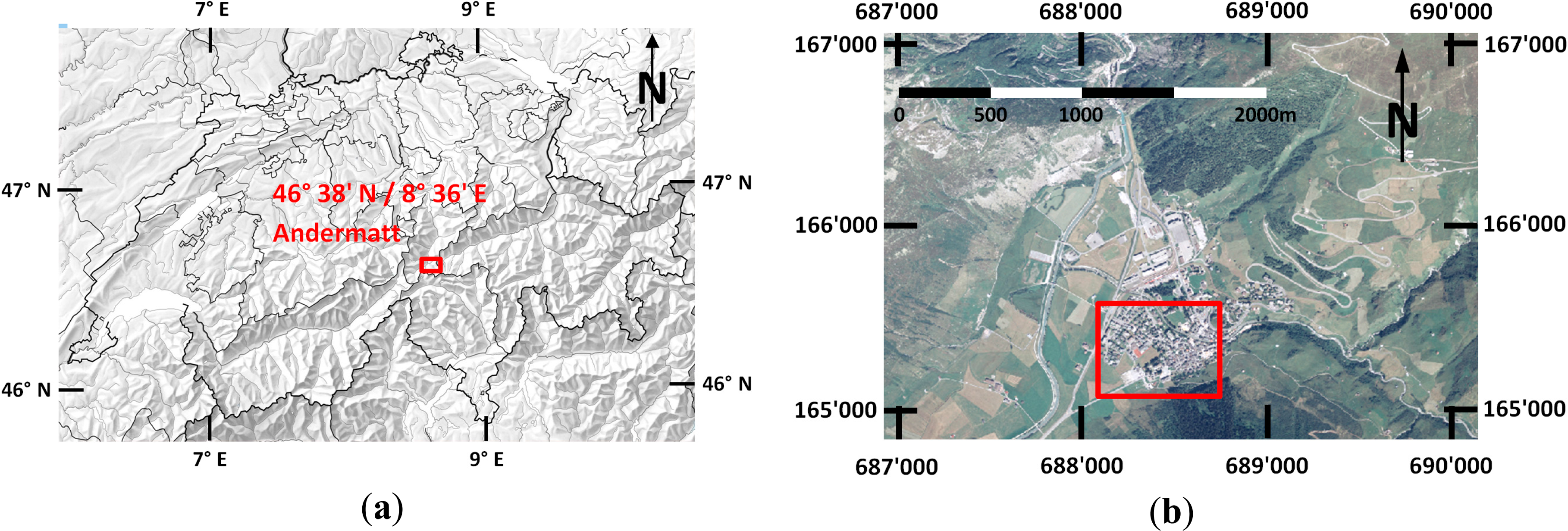
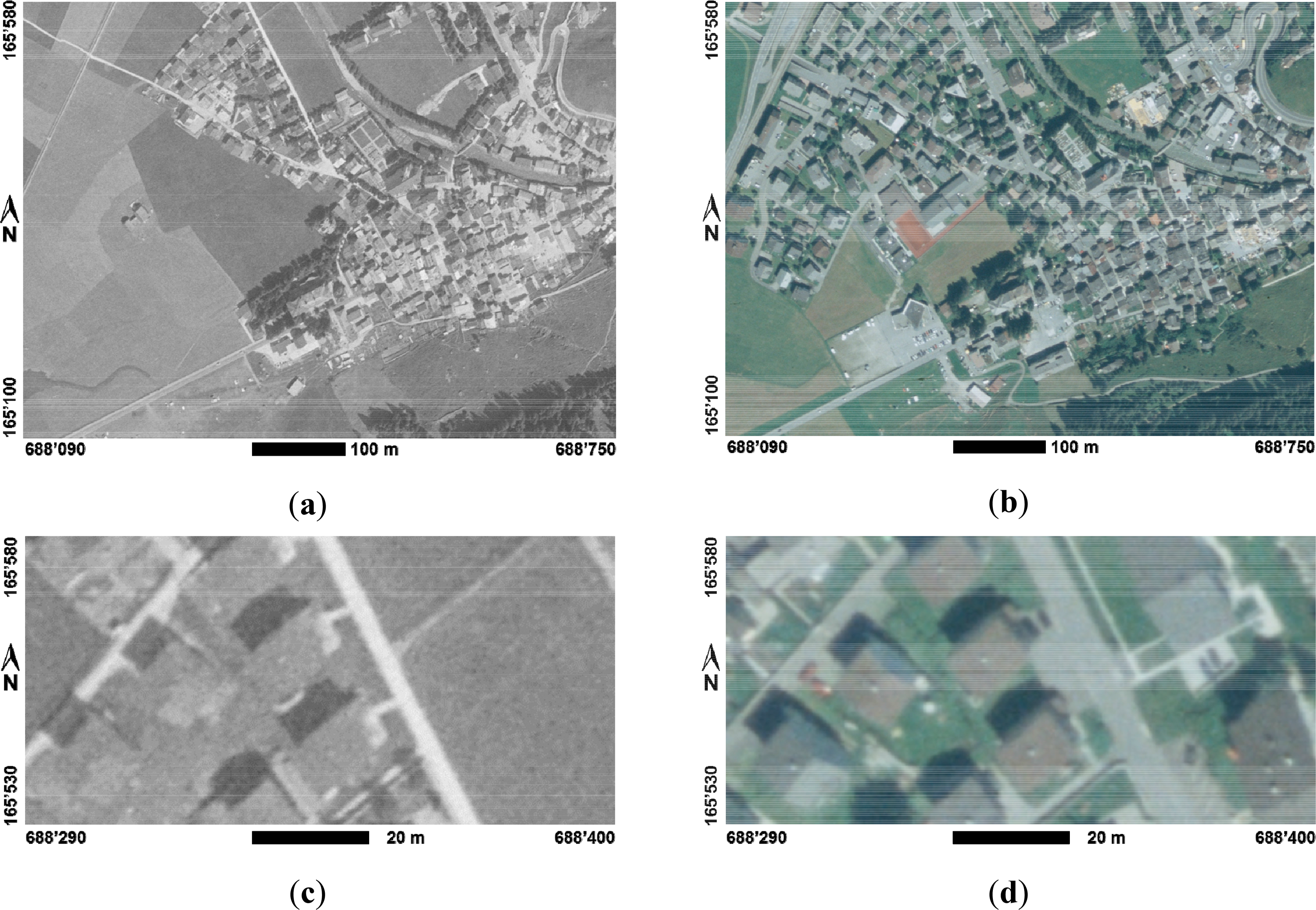
For the study, the alpine town and tourist resort of Andermatt was chosen. Andermatt is situated in Central Switzerland (Figure 1a) at an important traffic junction of the Alps—the Gotthard (N-S) and the Furka-Oberalp (E-W) routes. Andermatt and its surroundings served as study area in the earlier interdisciplinary project ProMeRe [11] with the goal of researching processes and methods for the collaborative spatial analysis and development. As part of the ProMeRe project OBIA methods had successfully been applied to a number of research questions related to tourism, landscape development and change detection [6]. Among the ProMeRe project partners was the Swiss National Mapping Agency Swisstopo which provided a very comprehensive series of historical and current geodata from their geospatial archives [24], including terrestrial and airborne imagery covering almost a century. For the following investigations the study area was limited to the built-up area of the actual town of Andermatt shown in Figure 2. The figure also illustrates the main characteristics of the area: buildings with mainly two to four floors and mostly gable roofs; numerous free-standing buildings often surrounded by large trees; rows of buildings along the main street in the old part of town.
3.2. Experimental Data
While the original time series of scanned historical aerial imagery of the study area encompasses six epochs, the following experiments were focusing on the earliest and the most recent epochs 1959 and 2007. Details of the aerial imagery used are listed in Table 1 and their visual characteristics are shown in Figure 2.
Figure 2a,b shows the extents of the study area as it was used in all the subsequent investigations and illustrations. The detail views in the lower row of Figure 2 illustrate the relatively poor contrast of both data sets, which in case of the grayscale imagery make the identification of buildings very difficult—even for a human observer. The aerial photographs were provided with calibration protocols for the respective cameras, thus, allowing the reconstruction of original interior camera orientation.
The experimental data for the study area also includes the following current geodata:
A LiDAR-based digital terrain model (DTM-AV) as part of the official cadastral survey of Switzerland with a grid spacing of 2 m and a nominal height accuracy of ± 0.5 m.
Building footprints from the official cadastral survey database to be used as input for the backdating process.
3.3. Reference Data
For our studies, two comprehensive reference data sets were available which had been collected as part of the earlier ProMeRe [11] project:
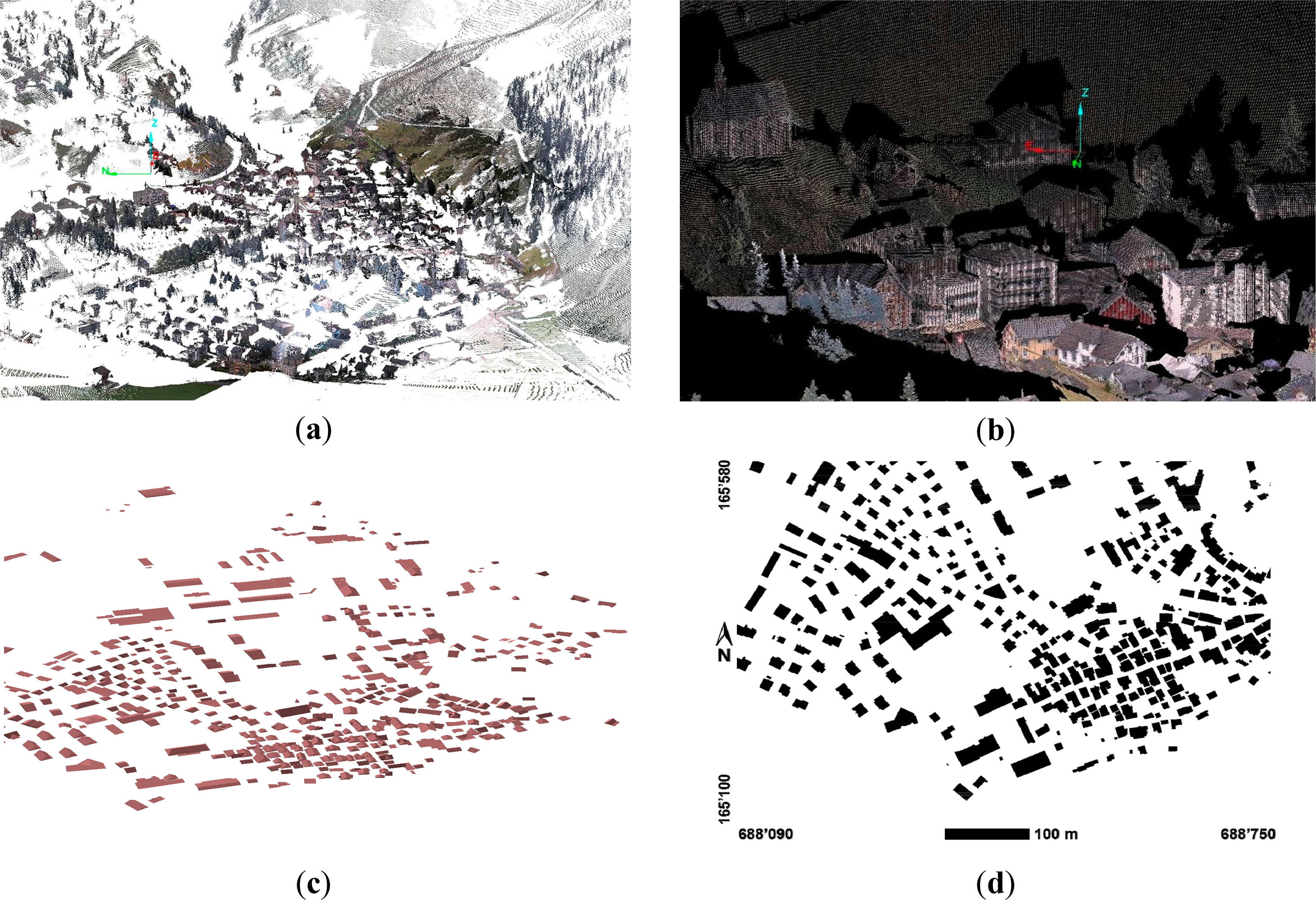
Oblique terrestrial laserscans (see Figure 3a,b) using a Leica HDS4400 long range scanner had been collected from six elevated scan positions around Andermatt [25]. The density of the point cloud data varies with distance and exposition towards scanning source but is generally in the order of 10–20 points per square meter. The average 3D point accuracy of the data in the town center is in the order of 10–20 cm [25]. This data set served as a reference for the evaluation of the extracted 3D point clouds and DSMs.
3D roof geometries (see Figure 3c) of all buildings in the study area had been collected manually by stereo restitution using ERDAS StereoAnalyst and Feature Assist for ArcGIS. This stereo restitution had been performed with imagery of all epochs including 1959 and 2007. The 3D roof geometry of each building was semi-automatically assigned to a building ID using the cadastral building footprint data (Figure 3d) and subsequently stored in a GIS database. In the subsequent experiments the roof geometry was used to evaluate the performance of the building detection process.
4. DSM Extraction from Historical Aerial Photographs
4.1. Image Matching Software
In our subsequent image matching experiments, three different image matching software packages were used—a feature-based sparse matching solution and two dense matching solutions:
LPS eATE is a DSM extraction module of the former ERDAS IMAGINE LPS product line (now: IMAGINE Photogrammetry). In the pre-2014 versions used, eATE incorporated a traditional feature-based sparse stereo matcher. (Note: as of 2014, eATE incorporates an implementation of the SGM algorithm [13]). Since LPS was designed for analog and digital aerial imagery, it supports the entire workflow from the reconstruction of the interior orientation of analog imagery, through bundle orientation and DSM extraction to orthoimage production.
Agisoft PhotoScan [26] is a software product originating from the computer vision domain and supporting the photogrammetric 3D reconstruction workflow for small to medium format digital imagery. PhotoScan incorporates a dense image matcher based on structure from motion (SFM) and other undisclosed multi-view stereo algorithms.
SURE [27] is a dense image matching software by the University of Stuttgart and its spin-off company nFrames [28]. SURE consists of modules for image rectification, dense image matching, 3D point cloud generation and triangulation. The dense image-matching module is based on the SGM algorithm by Hirschmüller [29].
Among the challenges of using multiple image matching solutions are their different inputs and outputs as illustrated by Cavegn et al. [30] and the fact that only LPS is currently supporting the full photogrammetric workflow for analog aerial imagery.
4.2. Georeferencing of the Analog Aerial Imagery
For the comparison of the results by the different image matchers, an accurate common georeference was to be established. The original strategy was to perform indirect georeferencing in one software solution, using ground control points and a bundle adjustment, and then to transfer the interior and exterior orientation parameters to the other two software solutions. However, due to partly undocumented, incompatible exterior orientations and lens distortion models, this strategy had to be modified. The solution for the 1959 and 2007 data sets consisted of:
- (a)
indirect reference orientations in LPS
- (b)
indirect image orientations in PhotoScan which were also applied to the input imagery for SURE
- (c)
transformation of the resulting dense 3D point clouds from PhotoScan and SURE to the sparse 3D point cloud of LPS in order to obtain co-registered DSMs for the subsequent investigations.
The reference orientations in LPS for the 1959 and 2007 imagery were carried out using a bundle adjustment with four images and with approx. 10 natural GCPs (ground control points) each. The reference orientation yielded average control point 3D RMS values in the order of 4 pixels GSD (1959: 2.7 m and 2007: 2.4 m). One of the limiting factors proved to be the identification of identical GCPs over a period of up to 50 years.
The co-registration of the generated DSMs was performed using an implementation of the iterative closest point (ICP) algorithm by Besl and McKay [31] in CloudCompare [32]. The ICP-based transformation of each densely matched 3D point cloud to the respective sparse 3D point cloud resulted in RMS values in the range of 5 m and maximum residuals in the order of 70–90 m. It should be noted that these figures represent 3D point-to-point distances, which are directly affected by the sparse and uneven point spacing of the sparse reference DSMs for 1959 and 2007 generated with eATE. Thus, the few but large residuals represent mainly horizontal difference vectors to points in particularly sparse areas of the eATE reference DSMs. Due to the very large number of points, i.e., ICP observations in the respective point clouds, the automatically generated transformation results are still acceptable. It should also be noted that the very steep and heavily vegetated area in the southeasterly (i.e., lower right) border of test area was excluded from the transformation. This results in cropped DSMs for the two dense matchers PhotoScan and SURE as shown, for example, in Figure 4c,e.
4.3. Discussion of Image-Based DSM Extraction Results
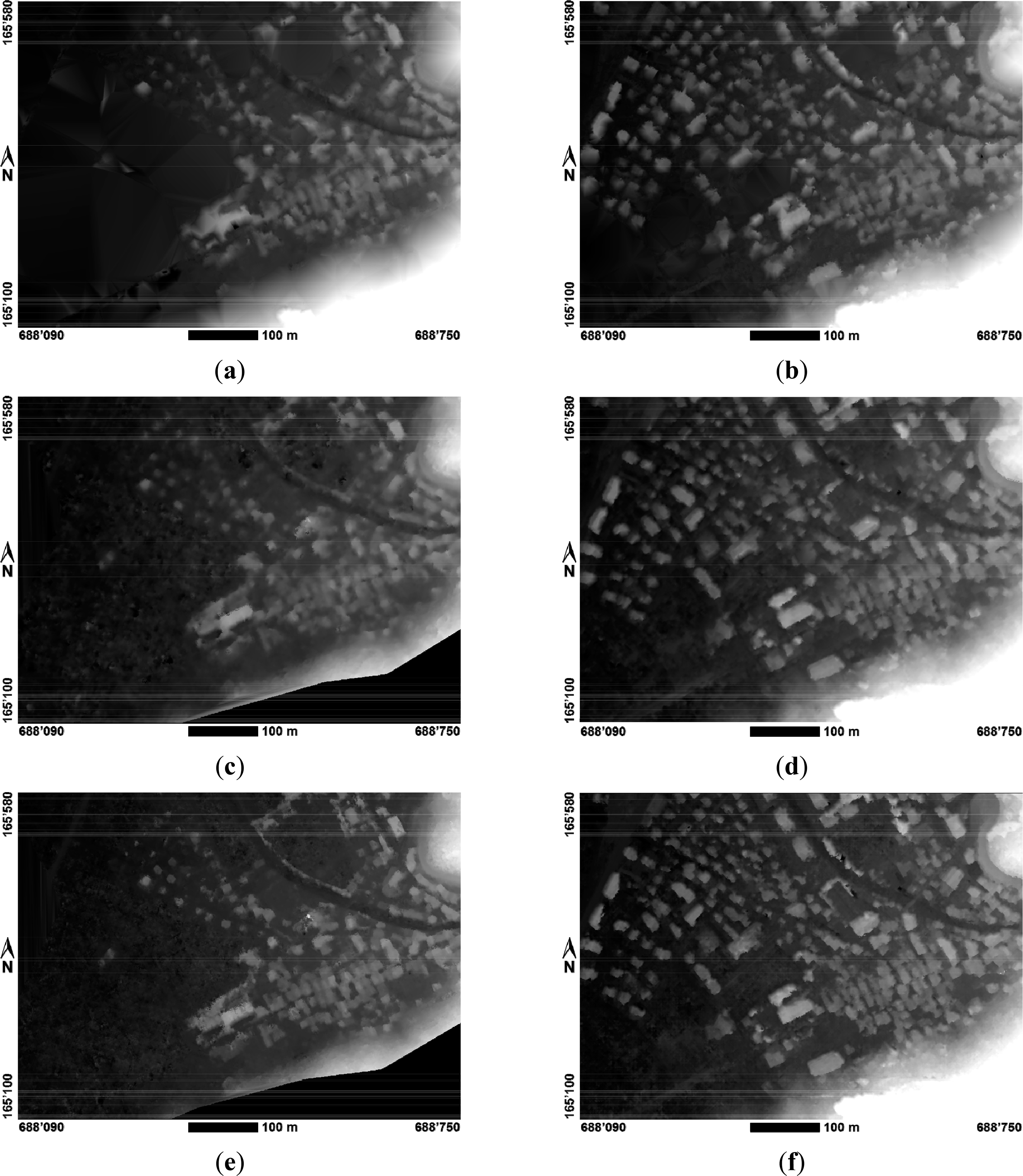
The image-based DSM extraction results from the three different image matching solutions are illustrated in Figure 4, with the DSMs derived from the 1959 imagery in the left column and the DSMs from the 2007 imagery in the right column. The comparison shows an increasing sharpness and level of detail, starting from the sparse matcher eATE in the top row, followed by the dense matchers PhotoScan in the middle row and SURE in the bottom row.
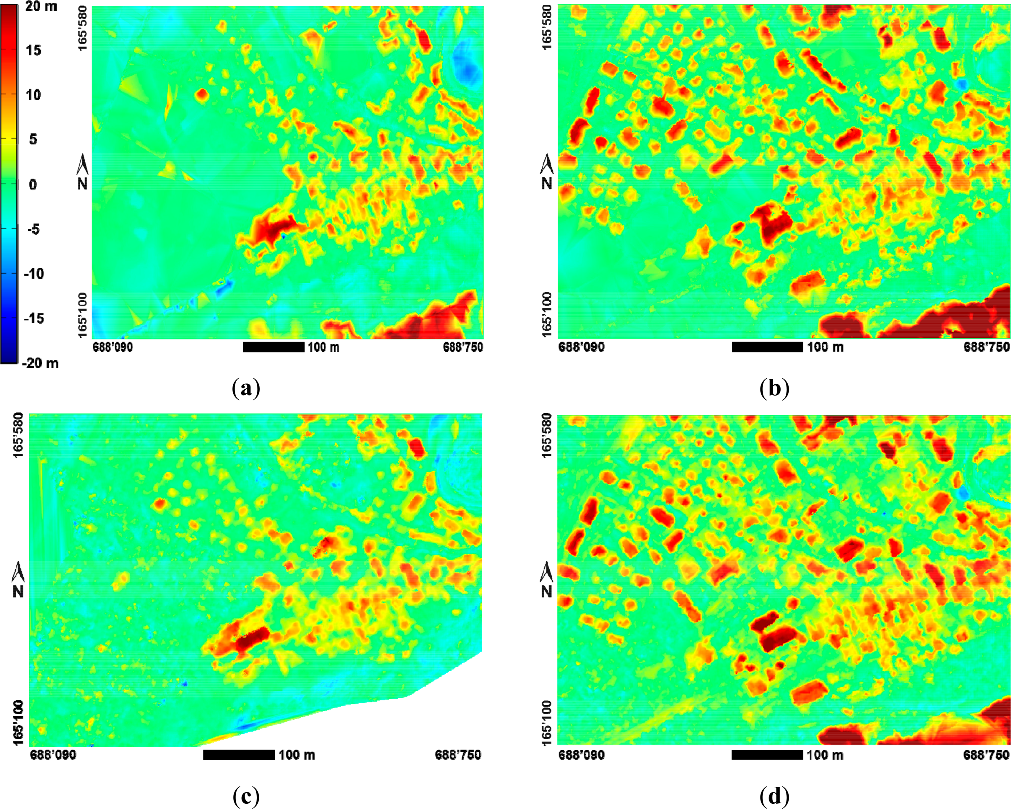
An even better comparison is offered by normalized digital surface models (nDSM) shown in Figure 5, which are calculated by subtracting the DTM (DTM-AV) from the respective DSM. Under ideal conditions, the nDSM should represent the heights of artificial or natural objects not belonging to the earth’s surface, e.g., buildings or vegetation. Figure 5 again shows the nDSMs extracted from the 1959 grayscale imagery in the left hand column and those extracted from the 2007 color imagery in the right hand column.
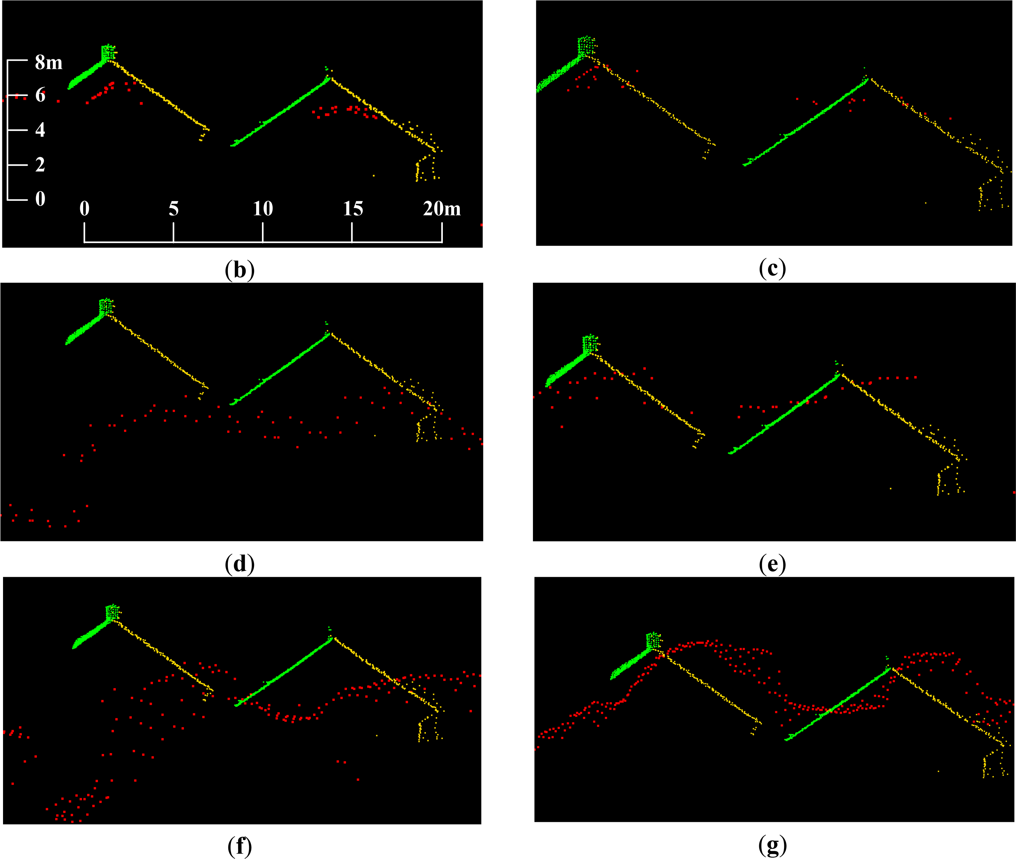
For a more detailed evaluation of the DSM quality, cross-sections of the DIM-based point clouds are compared with reference profiles from long-range oblique TLS. Such a profile comparison is shown in Figure 6. The visual inspection yields the following results: a reasonably good absolute orientation but poor level of detail of the sparsely matched eATE DSMs 1959 (Figure 6b) and 2007 (Figure 6c); a vertical and horizontal offset of the 1959 absolute orientations of the PhotoScan (Figure 6d) and SURE (Figure 6f) DSMs in the order of 4–5 m as well as a horizontal offset of the 2007 DSMs in the order of 3–4 m, which are clearly visible in (Figure 6g). These offsets are probably resulting from the current co-registration workaround described in the previous section. Finally, the very high point density and the high level of detail of the SURE DSM 2007 are shown in (Figure 6g).
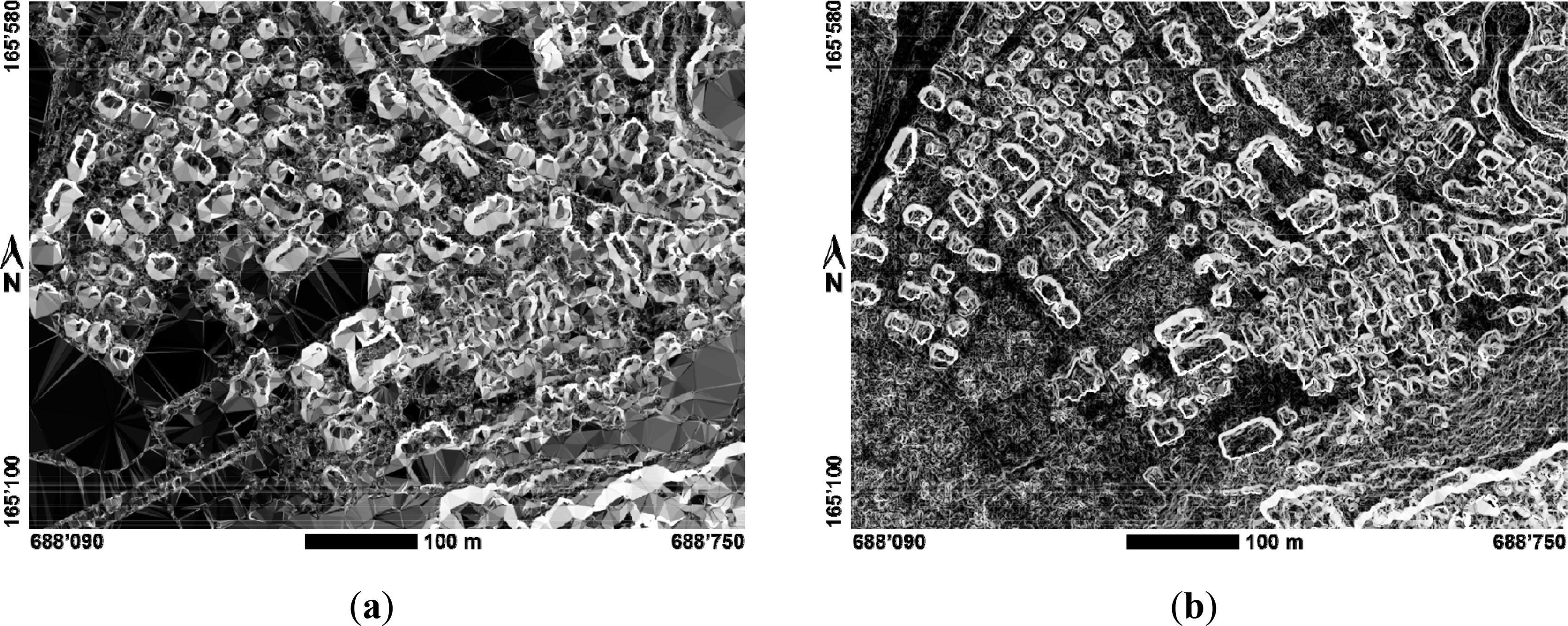
Figure 7 shows the gradients of the extracted DSMs for 2007. It illustrates the much sharper definition of the building edges within the densely matched DSM (SURE) shown in Figure 7b on the right in comparison to the sparsely matched DSM (eATE) in Figure 7a on the left. Finally, the examples of temporal DSM differences for sparsely and densely matched DSMs in Figure 8 demonstrate the additional potential of using densely matched DSMs for rapid visual and analytical landscape change analyses which were not further investigated within our study.
4.4. Discussion of DSM Extraction Quality
From the ongoing effort of establishing benchmarks for dense image matching algorithms in traditional and oblique airborne photogrammetry [12,15,33] a number of comparisons and suitable quality indicators have emerged. The following evaluation of point densities and accuracies based on point cloud scatter was carried out on the grounds of the methodology and tools developed by Deuber [33].
The point densities obtained with the SURE SGM-based dense matcher of 1.02 and 0.79 listed in Table 2 are close to the targeted value of 1 point per pixel for pixel-based matching–both for greyscale and color photographs. As expected, the point density provided by the sparse matcher eATE is much lower—in the order of 1/6 to 1/4 of the SGM density. The point densities obtained from PhotoScan are lower than expected. As shown by Deuber [33], similar point densities to those from SURE can be expected, when PhotoScan is applied to medium-format digital aerial imagery. However, even on high-end PC hardware, the large format aerial imagery of this project could not be processed with full, i.e., “very high” point density and had to be processed with reduced “high” density instead. Overall, it should be noted that state-of-the art dense image matching algorithms are capable of generating very high density DSMs with remarkable 2.5–2.7 points per square meter, even from historical aerial photographs.
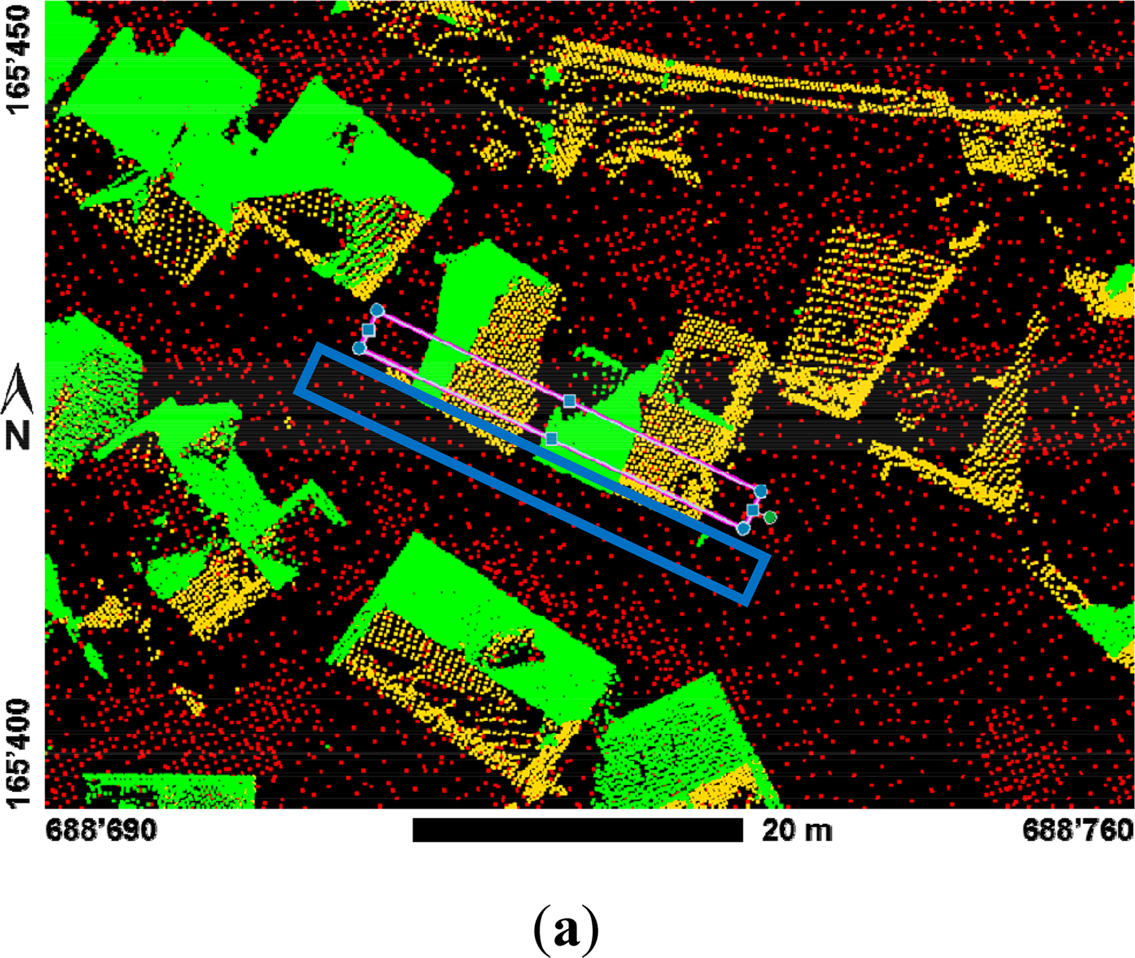
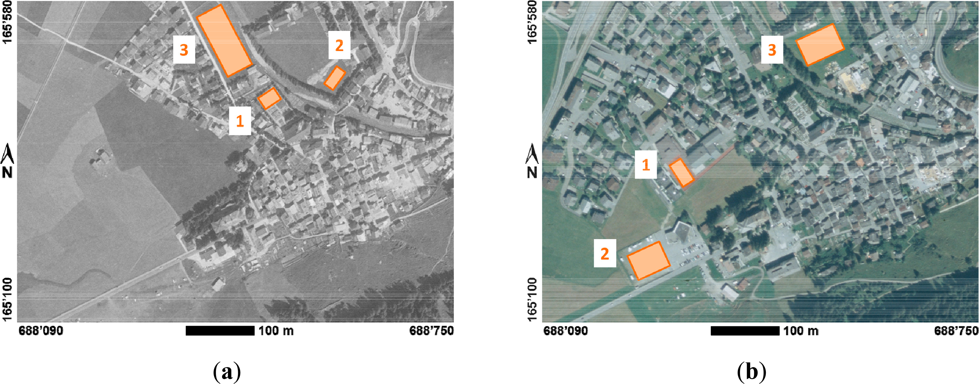
In a subsequent test the scatter of the respective densely matched DSMs was investigated as an indicator for relative DSM accuracy. In order to determine the scatter of the generated 3D point clouds, three planar test areas per epoch were identified (see Figure 9), approximating planes were estimated and the respective point-to-plane residuals were computed to provide the RMS errors (RMSE) and maximum errors shown in Table 3.
With the 1959 grayscale imagery, PhotoScan yielded DSMs with RMSE values between 0.29 m and 1.82 m and SURE with RMSE between 0.19 m and 1.08 m. This is equivalent to 0.5–2.8 GSD in the case of PhotoScan and 0.3–1.7 GSD in the case of SURE. With the 2007 imagery, PhotoScan delivered RMSE values between 0.48 m and 0.76 m and SURE yielded RMSE values between 0.47 m and 1.01 m. This corresponds to 0.9–1.4 GSD for PhotoScan and 0.9–1.8 GSD for SURE. In their dense matching tests with modern high-resolution digital airborne imagery, Haala and Rothermel [15] obtained RMSE values for planar soccer grounds well under 0.5 GSD. However, considering the fact that our tests were carried out with historical grayscale and color aerial photographs with a limited radiometric and spatial resolution, the RMSE values of the historic DSMs in the order of 1–1.5 GSD are quite remarkable.
5. DSM-Based Building Detection Using OBIA
5.1. Building Change Detection Strategy and Workflow
A suitable building change detection strategy largely depends on the goals and requirements of the targeted application. Our investigations are part of a long-term multi-disciplinary initiative [6,11] for monitoring and analyzing the historical and future development of alpine settlements and vegetation. Over the last 100 years, the development has been influenced by factors, such as tourism and agriculture—and, in certain areas, by the reduction of military forces. Within the initiative, the settlement development is analyzed from the different perspectives of historians, urban and territorial planners, as well as architects. The main characteristics and requirements of the settlement analysis in general and the building change detection in particular include:
The alpine settlement development over the last 100 years was dominated by the building or re-building of housing still in existence today with only few cases of major demolitions.
The process should be capable of detecting individual, identifiable buildings—not just changes in settlement areas—and should reliably deliver the epoch at which a building first appeared in one of the historic aerial images.
There is an existing official cadastral database including recent building footprints for large parts of Switzerland which could be used in relating detected buildings to current building identifiers.
The building change detection procedure should be robust and the results of the test area should be transferable to other alpine and rural regions.
As a consequence, a back-dating approach based on today’s building database was incorporated into the building change detection process based on the historical DSMs from dense image matching discussed above and on the OBIA-based building detection process outlined below. Since the building detection process is conducted for each generation of imagery independently, it also results in a complete time series of detected buildings at each epoch.
5.2. Our Earlier Building Detection Workflow
Prior to the proposed DIM-based workflow, a building detection process incorporating DSMs from conventional sparse image matching and OBIA methods had been developed by Meier and Walch [10]. This process is briefly introduced in order to permit a later assessment of the improvements offered by the new DIM-based approach.
The earlier workflow was developed using the same experimental data as listed in Section 3.2, with the difference that the imagery had included a total of six epochs between 1959 and 2007. The workflow included historical DSMs derived with an earlier version of the sparse image matching solution eATE. The coarse nature of the historical DSMs generated at the time—in combination with the poor quality of the historical imagery—originally resulted in many false positives in the building detection process. In the final workflow this was successfully improved by the following two main measures:
The incorporation of a shadow detection process (based on IMAGINE Objective’s “Association Shadow” function), which allowed eliminating erroneous nDSM height cues resulting from DSM matching and interpolation errors and not from actual building geometries. While the shadow detection process works well for isolated buildings it suffers in dense built-up areas and in areas where buildings are intertwined with large trees.
The integration of the cadastral building database into the OBIA-based detection process—and not just in the final back-dating process. This prevents the process from detecting buildings which had potentially existed and which had since been demolished.
With this process, a building detection rate of 88% was achieved [10]. However, the process is very time consuming and complex and lacks robustness and transferability, for example, due to manual adjustments of the association shadow settings. These settings require knowledge about image acquisition date and time, which might not be available for historic imagery.
5.3. New OBIA Workflow Incorporating DSM from Dense Image Matching
Among the main innovations of the new workflow shown in Figure 10 are the incorporation of the high-resolution historical DSMs from dense image matching and the integration of the new segmentation algorithm (Full Lambda Schedule Algorithm) [34] implemented in IMAGINE Objective.
The key elements of the DIM- and OBIA-based workflow are the following. First, training areas are chosen for buildings and for non-residential areas, i.e., classification background, including forest, rivers, trees, roads, fields, gardens, gravel spaces, etc. (see examples in Figure 11). Next, the ortho imagery derived from the historical imagery is segmented based on defined training areas in IMAGINE Objective using the ‘Segmentation Lambda Scheme’ [34] in which spectral, textural, size and shape properties can be weighted individually. The resulting potential housing segments are filtered with a size and a probability filter, which eliminates small segments and segments with a low probability for housing.
Normalized DSMs (nDSM) are generated for each epoch by subtracting the recent DTM from the respective historical DSM. Next, an upper and lower threshold is applied to the nDSM in order to extract significant height differences, i.e., potential object elevations above ground. The lower threshold value is used to exclude small height differences created by DSM noise, minor changes to the terrain, low growing vegetation, and small structures, such as parked cars and sheds. The upper threshold can be used to exclude gross errors and tall trees common to alpine areas.
Intersection of nDSM and image segmentation—In a rule-based approach the filtered segments are combined with the nDSM. Thus, all pixels with high probability for the class buildings and with height differences within the threshold values are selected.
Vectorization and Cleaning—The resulting pixel segments are then cleaned by means of morphological operations (dilation, erosion), reclumped and vectorized. An additional Island Filter is applied to eliminate holes in the resulting polygons.
The subsequent backdating is conducted in ArcGIS by spatially joining the output polygons from the vectorization and cleaning process with the building footprints of the cadastral survey database. If a polygon matches a building, then the building is being marked as existing at the given epoch and a time stamp is written to the attribute table. Polygons not matching any building in the database are an indication for possible false positives or demolished buildings.
As part of our study, the quality of the building detection process is evaluated by comparing the detected buildings with the reference 3D roof data collected with stereo restitution using the same historical imagery. The results obtained in these experiments and the building detection accuracies achieved are discussed in the following sections.
5.4. Discussion of OBIA Building Detection Results
The building detection experiments were carried out using the three data sets listed in Table 4. Grayscale ortho images for 1959 and color ortho images for 2007 were derived from the original aerial images described in Section 3.2, using the LiDAR-based DTM (DTM-AV), as basis for the image rectification. In order to evaluate the influence of sparse versus dense image matching, DSM extraction results from the sparse image matcher eATE (LPS 2013) and from the dense image matcher SURE were chosen for each epoch. In order to exploit the DSMs in the OBIA software ERDAS Objective, they were first converted to a regular grid.
Training areas for the subsequent segmentation process were chosen for each epoch (see Figure 11). The selection of suitable training areas is an important factor for a successful segmentation and is the only part of the workflow which is specific to each epoch. While some training sites can be re-used over several epochs, re-definitions are frequently required due to land cover changes such as shown in Figure 11.
Segmentation—For the segmentation of the historical imagery we employed the Segmentation Lambda Schedule Filter which has recently been added to ERDAS Objective based on the Full Lambda Segmentation Algorithm (FLSA) by Redding et al. [34,35]. FLSA is a bottom up region merging algorithm aiming at minimizing the Mumford-Shah energy functional. In ERDAS Objective the merge cost function incorporates spectral information as well as segment’s texture, size and shape. Furthermore, the pixel per segment ratio, i.e., the average number of pixels per output segment, as well as minimum and maximum segment size constraints can be defined.
The selection of optimal segmentation parameters depends on the geometric and radiometric characteristics of the imagery and requires a certain amount of trial and error, as well as user experience. In our case a pixel per segment ratio of 500 in combination with high relative weights of 0.8 for the spectral and texture parameters and low weights of 0.2 for the parameters size and shape were used. The segmentation results obtained are shown in Figure 12a,b. The individual weights proved to be particularly valuable for separating trees from buildings. Their differentiation based on height (nDSM) only would otherwise be difficult, especially in greyscale imagery.
Intersection of normalized DSMs with segmentation results—Before the nDSM was intersected with the segmentation results, the optimal lower and upper thresholds were determined. These thresholds are mainly influenced by the quality of the historical DSMs. For our test area and data, a lower threshold of 3 m proved to be suitable in order to filter out DSM noise and small artifacts as well as low vegetation and small structures. An upper threshold of 25 m was chosen, since there were no taller buildings in the area and since it also allowed to reliably eliminating large fir trees which are common to the area. A disadvantage of setting the lower threshold at the chosen height difference is that this erodes the size and shape of the nDSM blob representing one or more buildings.
The results of the raw, pixel-based intersection results for the different nDSMs with the segmentation results for 1959 and 2007 are shown in Figure 13. The results for 1959 (left column, Figure 13a,c), being based on greyscale imagery, are clearly more fragmented than those for 2007 (right column, Figure 13b,d), which were derived from color photographs. The results based on densely matched DSMs (lower row, Figure 13c,d) yield a larger number of building candidate segments with contours that are generally better defined than in the results based on sparse DSM matching (upper row, Figure 13a,b).
Vectorization and Cleaning—For further processing, the raw pixel segments resulting from the intersection operation were first morphologically filtered using “dilate” and “erode” functions in order to obtain coherent individual building segments with optimal shape. These filtered pixel segments were then vectorized and an “island filter” was subsequently applied to the vector objects in order to eliminate holes within the polygons.
The output of the filtering and vectorization step is illustrated in Figure 14. A visual inspection of the 1959 results reveals many missing, i.e. “unmarked” small buildings in the upper left quadrant of Figure 14a for the sparse image matcher with a significant improvement in Figure 14c showing the result based on the densely matched DSM. For the 2007 data in Figures 14b,d, the visual differences between the two matching solutions are much smaller. In all cases, no individual buildings are recognizable in the densely built-up area of the town center (lower right quadrant). Therefore, additional processing steps are required, if individual buildings are to be detected—as specified in Section 5.1—and not just changes in settlement areas.
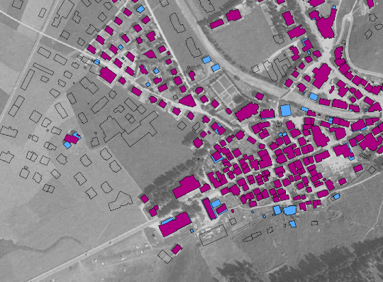
Backdating—The candidate building areas shown in were subsequently spatially joined with the building layer of the cadastral database in order to determine the existence of individual buildings at a specific epoch. The final results of our building detection process after the backdating step are illustrated in Figure 15.
Figure 15 shows the detected buildings in purple (sparse matching input) and dark red (dense matching input) overlayed onto the footprints of the current building database and the orthoimage of the respective epoch. For illustration purposes only, the results are also overlayed onto the 3D building reference data shown in light blue. This allows for visually highlighting undetected buildings (false negatives) present in the reference data—but not footprints incorrectly identified as buildings (false positives), since this information is covered by the respective layers of extracted buildings (in purple or dark red). While the number of false positives is very small (see following section), numerous false negatives occur. They are well visible in the 1959 data sets and in particular in the upper left quadrant of Figure 15a with the extraction results based on the sparsely matched DSM obtained with eATE. The SURE DSM workflow shows significantly better results for both epochs.
5.5. Discussion of Building Detection Accuracies
For the evaluation of the building detection quality, all buildings present in the 1959 and 2007 aerial imagery were manually digitized using stereoscopic restitution. As part of this process, the collected 3D roof geometry was grouped into building objects using Feature Assist for ArcGIS and stored in the GIS. The 3D roof geometry of these building objects served as reference data for the following evaluation of the detection quality. The resulting statistics for 1959 are listed in Table 5; those for 2007 are shown in Table 6.
The reference data for 1959 includes 258 buildings, of which 212 true positives were correctly detected by the process using the eATE sparse matching DSM and 236 by the one using the SURE dense matching DSM. 46 buildings in existence at the time had not been detected (false negatives) by the process based on the eATE DSM and 22 by the process based on the DSM generated with SURE. Both approaches yielded a very low rate of incorrectly detected buildings (false positives) of 3 and 7 buildings respectively. Thus, the results for 1959 show a detection rate (i.e., a completeness or producer’s accuracy) of 82% for the sparsely matched eATE DSM input and 92% for the densely matched SURE DSM input with very high correctness rates (i.e., precision or user’s accuracy) of 99% and 97% respectively.
In 2007 the identical test area included 357 buildings. The building detection process using a sparsely matched DSM input yielded 323 true positives, 34 false negatives and only two false positives, corresponding to a detection rate of 91% and a correctness of 99%. The process based on densely matched DSM input produced 335 correct detections, 22 false negatives and three false positives with a detection rate of 94% and a correctness of also 99%.
For the grayscale imagery of 1959 and the color imagery of 2007 there is a significant improvement of the building detection rate from sparsely matched DSM input to densely matched DSM input: for 1959 an improvement from 82% to 92% and, for 2007, an improvement from 91% to 94%. This corresponds to a major reduction of the FN rate to less than half, from 18% to 8% for the 1959 grayscale imagery and by a third from 9% to 6% for the 2007 color imagery. A closer inspection of the false negatives reveals that in the 2007 imagery only 5 buildings with an area of >25 m2 had not been detected. All the other false negatives were caused by undetected small buildings such as cabins or carports, etc. which are contained in the cadastral building database for legal reasons. Thus, if considering main buildings only, the detection rate would be significantly higher. The very high correctness rate of around 99% is mainly due to the backdating process which only accepts building candidates overlapping the footprints of the current cadastral building database.
Our results compare well with those listed in Section 2.2, in particular with related work by [22,23] which is also based on aerial imagery. However, a direct comparison is difficult for a number of reasons: first, our goal of tracing the first occurrence of each building in historical aerial imagery is different from that of other reviewed applications; second, our approach adds a backdating step and assumes the availability of a recent building database which makes the detection process more robust than a global search process and thus leads to a significantly lower FP rate. Last but not least, unlike in the other cases using fairly recent aerial imagery, some of our results are obtained from historical aerial photographs which were captured more than half a century ago.
Of particular relevance and interest is a direct comparison with the results from earlier work at our Institute by Meier and Walch [10]. Their research had focused on the same goals and had used the same test data, but their building detection process was based on sparsely matched DSM input since dense image matching was not yet available at the time. The average building detection rate achieved in their studies was 88%. In case of our sparsely matched DSM inputs, i.e., our eATE solutions, the detection rate was reduced to 82% for the 1959 imagery and improved to 91% for the 2007 imagery. This mixed outcome is an indication that the earlier building detection process largely relied on the associated shadow model and the direct use of the building database (see also Section 5.2). Both components were removed from the new approach in order to improve its robustness and transferability.
However, our main motivation was to investigate the influence of the newly introduced DSMs from dense image matching with the hypothesis, that their use would substantially improve the performance of building detection in historical aerial imagery. A comparison with the results of Meier & Walch [10] shows significant improvements in the building detection rate from the earlier 88% to 92% for grayscale imagery and to 94% for color imagery. This improved performance of the new approach is complemented by a substantial simplification and further automation of the new process, leading to major time and cost savings compared to the original solution.
6. Conclusions
In this article we introduced a novel approach for building detection and building change monitoring based on historical aerial photographs and object-based image analysis. The new approach uses DSMs extracted from the historical imagery using dense image matching together with the actual imagery itself as inputs to an OBIA process. Additional inputs include a current DTM from any suitable source and a current building database, which is used to identify individual buildings and to automatically record their first appearance in the historical imagery. In combination with emerging regional or national historical aerial image archives, this allows establishing a spatio-temporal building database dating back well over half a century with a very high level of automation. The new building detection process yielded a detection rate of 92% for the 1959 historical grayscale imagery and of 94% for the 2007 color imagery.
With this first systematic study on image matching with historical aerial imagery we demonstrated that dense DSMs can successfully be extracted both from greyscale and color photographs. The extracted historical DSMs show point densities of 2.5 to 2.7 points per m2 which are similar to recent airborne LiDAR DSMs and RMSE values in the order of 1 pixel GSD. These findings are remarkable, since dense image matching algorithms were originally developed for digital imaging sensors with high dynamic range and large image overlaps and since the low signal-to-noise ratio of the historical imagery makes the reliable identification and delineation of buildings a challenging task—even for human operators.
The presented combination of historical DSMs from dense image matching with state-of-the-art OBIA methods offers unique opportunities for exploiting archives of historical aerial photographs, which provide a uniquely rich memory of our environment—in some cases over almost a century. The DSM extraction capabilities demonstrated in this paper cannot only be applied to building change detection but to the reconstruction of historical 3D landscapes in general, thus, offering further opportunities in landscape change monitoring.
The building detection results demonstrated in this paper leave room for further improvement. The main limiting factor within our experiments is the georeferencing accuracy of the DSMs extracted from the different epochs of aerial imagery (see Section 4.2 and Figure 6). The accurate georeferencing of historical aerial imagery is generally a very challenging process—even if camera calibration values are available. This is mainly due to the difficulty of identifying natural control points that can still be localized today and subsequently measured in three dimensions. Once the exterior orientations of a set of historical images have successfully been reconstructed using a suitable photogrammetric software, users are faced with the problem that the majority of dense image matching software originates from computer vision and was originally developed for images from small to medium format digital sensors only. Thus, they usually do not support the reconstruction of the interior orientation of analog imagery using fiducial marks and quite often, they also do not support advanced lens distortion models required and used in airborne photogrammetry. However, with the addition of SGM-based dense image matching to photogrammetric software packages (e.g., LPS eATE 2014) and with the addition of advanced lens distortion models to dense matching software (e.g., to SURE), it is expected that the ICP-based georeferencing workaround used in this study will no longer be required. And due to the better absolute georeferencing accuracies of the extracted DSMs, the building detection rates are likely to be further improved in the future.
Acknowledgments
We would like to thank the Swiss Commission for Technology and Innovation CTI for supporting the original research ProMeRe (Project Number 9929.1) and all the project partners and members for their support. We would particularly like to thank the ProMeRe project partner Swiss Federal Office of Topography (swisstopo) for providing the historical aerial imagery used in this study. We would also like to acknowledge the support by Eric Matti and Kevin Hilfiker in carrying out parts of the experiments and in preparing some of the figures.
Author Contributions
Stephan Nebiker designed the overall research and wrote the majority of the paper. Natalie Lack designed, performed and analyzed the OBIA aspects of the research and contributed to the respective paper sections. Marianne Deuber performed and evaluated the experiments on dense image matching and contributed to the respective sections.
Conflicts of Interest
The authors declare no conflict of interest.
References
- Swisstopo–Bundesamt für Landestopografie. LUBIS-Viewer. Geodata-News. Available online: http://www.swisstopo.admin.ch/internet/swisstopo/en/home/apps/lubis.html (accessed on 27 August 2014).
- Simpson, J.W.; Boerner, R.E.J.; DeMers, M.N.; Berns, L.A.; Artigas, F.J.; Silva, A. Forty-eight years of landscape change on two contiguous Ohio landscapes. Landsc. Ecol 1994, 9, 261–270. [Google Scholar]
- Walde, I. Zeitreihenanalyse historischer und aktueller Luftbilder. In Proceedings of the AGIT Symposium und Fachmesse für Angewandte Geoinformatik, Salzburg, Austria; July 2009; pp. 8–10. [Google Scholar]
- Kadmon, R.; Harari-Kremer, R. Studying long-term vegetation dynamics using digital processing of historical aerial photographs. Remote Sens. Environ 1999, 68, 164–176. [Google Scholar]
- Fensham, R.J.; Fairfax, R.J. Aerial photography for assessing vegetation change: A review of applications and the relevance of findings for Australian vegetation history. Aust. J. Bot 2002, 50, 415–429. [Google Scholar]
- Lack, N.; Bleisch, S. Object-based change detection for a cultural-historical survey of the landscape—From cow trails to walking paths. In Proceedings of the GEOBIA 2010: Geographic Image Analysis, Ghent, Belgium, 29 June–2 July 2010.
- Oczipka, M. Objektbasierte Klassifizierung hochauflösender Daten in urbanen Räumen unter besonderer Berücksichtigung von Oberflächenmodellen. Ph.D. Thesis, Freie Universität, Berlin, Germany. 2007. [Google Scholar]
- Klink, A.; Lücke, C.; Völker, A.; Höke, S.; Rolf, M. Semiautomatische Luftbildauswertung zur Erfassung von Siedlungs-und Verkehrsflächen als Unterstützung des nachhaltigen Flächenmanagements. Photogramm. Fernerkund. Geoinf 2008, 5, 441–451. [Google Scholar]
- Dini, G.R.; Jacobsen, K.; Rottensteiner, F.; Al Rajhi, M.; Heipke, C. 3D building change detection using high resolution stereo images and a GIS database. Int. Arch. Photogramm. Remote Sens. Spat. Inf. Sci 2012, XXXIX-B7, 299–304. [Google Scholar]
- Meier, A.; Walch, M. Objektbasierte Veränderungsanalyse und automatische Objektzuordnung am Beispiel der Siedlungsentwicklung. Bachelor Thesis, FHNW University of Applied Sciences and Arts Northwestern Switzerland, Muttenz, Switzerland. 2010. [Google Scholar]
- Bleisch, S.; Scheuerer, S. Räumlich-zeitliches Datenmanagement am Fallbeispiel kulturhistorischer Analyse der touristischen Entwicklung in Andermatt (CH). GIS Sci. 2012, 4, 146–154. [Google Scholar]
- Haala, N. The Landscape of Dense Image Matching Algorithms. In Photogrammetric Week ’ 13; Fritsch, D., Ed.; Wichmann: Stuttgart, Germany, 2013; pp. 271–284. [Google Scholar]
- Hirschmüller, H. Accurate and efficient stereo processing by semi-global matching and mutual information. In Proceedings of the 2005 IEEE Computer Society Conference on Computer Vision and Pattern Recognition (CVPR ’05), San Diego, CA, USA, 20–26 June 2005; 2, pp. 807–814.
- Heipke, C. Performance and state-of-the-art of digital stereo processing. In Photogrammetric Week ’93; Fritsch, D., Hobbie, D., Eds.; Wichmann: Stuttgart, Germany, 1993; pp. 173–183. [Google Scholar]
- Haala, N.; Rothermel, M. Dense multi-stereo matching for high quality digital elevation models. Photogramm. Fernerkund. Geoinf 2012, 4, 331–343. [Google Scholar]
- Blaschke, T. Object based image analysis for remote sensing. ISPRS J. Photogramm. Remote Sens 2010, 65, 2–16. [Google Scholar]
- Doxani, G.; Siachalou, S.; Tsakiri-Strati, M. An object-oriented approach to urban land cover change detection. Int. Arch. Photogramm. Remote Sens. Spat. Inf. Sci 2008, 37, 1655–1660. [Google Scholar]
- Doxani, G.; Karantzalos, K.; Strati, M.T. Monitoring urban changes based on scale-space filtering and object-oriented classification. Int. J. Appl. Earth Obs. Geoinf 2012, 15, 38–48. [Google Scholar]
- Chaabouni-Chouayakh, H.; Krauss, T.; Reinartz, P. 3D change detection inside urban area using different digital surface models. Int. Arch. Photogramm. Remote Sens. Spat. Inf. Sci 2010, 38, 86–91. [Google Scholar]
- Tian, J.; Reinartz, P. Multitemporal 3D change detection in urban areas using stereo information from different sensors. In Proceedings of the International Symposium on Image and Data Fusion (ISIDF), Tengchong, China, 9–11 August 2011; pp. 1–4.
- Tian, J.; Cui, S.; Reinartz, P. Building change detection based on satellite stereo imagery and digital surface models. IEEE Trans. Geosci. Remote Sens 2014, 52, 406–417. [Google Scholar]
- Gladstone, C.S.; Gardiner, A.; Holland, D.A. Semi-automatic method for detecting changes to ordnance survey topographic data in rural environments. In Proceedings of the 4th GEOBIA, São José dos Campos, Brazil, 7–9 May 2012; pp. 396–401.
- Jung, F. Detecting building changes from multitemporal aerial stereopairs. ISPRS J. Photogramm. Remote Sens 2004, 58, 187–201. [Google Scholar]
- Rickenbacher, M. Journeys through time with the Swiss national map series. In Proceedings of the 26th International Cartographic Conference, Dresden, Germany, 25–30 August 2013.
- Abt, L. LEICA HDS 4400-Aufnahme, Auswertung und Evaluation im ProMeRe-Projektgebiet Andermatt. Bachelor Thesis, FHNW University of Applied Sciences and Arts Northwestern Switzerland, Muttenz, Switzerland,. 2009. [Google Scholar]
- Agisoft PhotoScan, Professional edition Available online: http://www.agisoft.ru/products/photoscan/professional/ (accessed on 29 March 2014).
- Wenzel, K.; Rothermel, M.; Fritsch, D. SURE–The ifp software for dense image matching. In Photogrammetric Week ’13; Fritsch, D., Ed.; Wichmann: Stuttgart, Germany, 2013; pp. 59–70. [Google Scholar]
- Rothermel, M.; Wenzel, K. SURE–Photogrammetric surface reconstruction from imagery. In Proceedings of the LC3D Workshop, Berlin, Germany, 4–5 December 2012.
- Hirschmüller, H. Stereo processing by semiglobal matching and mutual information. IEEE Trans. Pattern Anal. Mach. Intell. 2008, 30, 328–341. [Google Scholar]
- Cavegn, S.; Nebiker, S.; Deuber, M. Dense Image Matching mit Oblique Luftbildaufnahmen–Ein systematischer Vergleich verschiedener Lösungen mit Aufnahmen der Leica RCD30 Oblique Penta. In Geoinformationen öffnen das Tor zur Welt, Gemeinsame Tagung 2014 der DGfK, der DGPF, der GfGI und des GiN (DGPF Tagungsband 23); Seyfert, E., Gülch, E., Heipke, C., Schiewe, J., Sester, M., Eds.; DGPF: Potsdam, Germany, 2014. [Google Scholar]
- Besl, P.J.; McKay, H.D. A method for registration of 3-D shapes. IEEE Trans. Pattern Anal. Mach. Intell 1992, 14, 239–256. [Google Scholar]
- Girardeau-Montaut, D. CloudCompare-3D Point Cloud and Mesh Processing Software, 2014. Cloud Compare. Available online: www.cloudcompare.org (accessed on 29 March 2014).
- Deuber, M. Oblique Photogrammetry: Dense Image Matching mit Schrägluftbildern. Master Thesis, FHNW Institutee of Geomatics Engineering, University of Applied Science and Arts Northwestern Switzerland, Muttenz, Switzerland,. 2014. [Google Scholar]
- Redding, N.J.; Crisp, D.J.; Tang, D.; Newsam, G.N. An efficient algorithm for Mumford-Shah segmentation and its application to SAR imagery. In Proceedings of the 1999 Conference on Digital Image Computing: Techniques and Applications (DICTA-99), Perth, WA, Australia, 7–8 December 1999; pp. 35–41.
- Crisp, D.J.; Perry, P.; Redding, N.J. Fast segmentation of large images. In Proceedings of the 26th Australasian Computer Science Conference, Adelaide, SA, Australia, 4–7 February 2003; pp. 87–93.


| Year | Imagery | Camera/Sensor | Image Scale | Avg. GSD |
|---|---|---|---|---|
| 1959 | analog, grayscale, 1 strip with 4 images, 80% overlap (scanned at 21 µm resolution) | Wild RC5, frame camera, 18 cm × 18 cm, c = 115.26 mm | 1: 30,000 | 64 cm |
| 2007 | analog, color, 1 strip with 4 images, 80% overlap (scanned at 13 µm resolution) | Leica RC30, frame camera, 23 cm × 23 cm, c = 152.51 mm | 1: 39,000 | 54 cm |
| [points/m2] ([points/pixel]) | 1959 | 2007 |
|---|---|---|
| eATE | 0.41 (0.17) | 0.71 (0.21) |
| PhotoScan (*) | 0.77 (0.31) | 0.67 (0.20) |
| SURE | 2.49 (1.02) | 2.72 (0.79) |
| Area | 1959 (GSD 0.64 m) | 2007 (GSD 0.54 m) | |||
|---|---|---|---|---|---|
| PhotoScan | SURE | PhotoScan | SURE | ||
| 1 | # of points | 708 | 2235 | 764 | 3215 |
| RMS (m) | 0.29 | 0.19 | 0.48 | 0.47 | |
| Max. error (m) | 1.45 | 1.12 | 2.40 | 1.81 | |
| 2 | # of points | 510 | 1727 | 1198 | 5189 |
| RMS (m) | 1.82 | 0.84 | 0.56 | 0.64 | |
| Max. error (m) | 7.54 | 3.54 | 2.20 | 2.36 | |
| 3 | # of points | 1345 | 5308 | 1942 | 7444 |
| RMS (m) | 1.37 | 1.08 | 0.76 | 1.01 | |
| Max. error (m) | 10.09 | 6.99 | 2.53 | 3.24 | |
| Year | Ortho Imagery | DSM (GSD) | DTM (GSD) | |
|---|---|---|---|---|
| (Color Bands and GSD) | eATE | SURE | DTM-AV | |
| 1959 | 1 band greyscale, GSD 50 cm | 50 cm | 50 cm | 2 m |
| 2007 | 3 band RGB, GSD 44 cm | 35 cm | 50 cm | |
| 1959 | Total # Buildings | True Positives (TP) | False Positives (FP) | False Negatives (FN) | True Negatives (TN) | Detection Rate | Correctness |
|---|---|---|---|---|---|---|---|
| eATE | 258 | 212 | 3 | 46 | 114 | 82% | 99% |
| SURE | 258 | 236 | 7 | 22 | 110 | 92% | 97% |
| 2007 | Total # Buildings | True Positives (TP) | False Positives (FP) | False Negatives (FN) | True Negatives (TN) | Detection Rate | Correctness |
|---|---|---|---|---|---|---|---|
| eATE | 357 | 323 | 2 | 34 | 16 | 91% | 99% |
| SURE | 357 | 335 | 3 | 22 | 15 | 94% | 99% |
© 2014 by the authors; licensee MDPI, Basel, Switzerland This article is an open access article distributed under the terms and conditions of the Creative Commons Attribution license (http://creativecommons.org/licenses/by/3.0/).
Share and Cite
Nebiker, S.; Lack, N.; Deuber, M. Building Change Detection from Historical Aerial Photographs Using Dense Image Matching and Object-Based Image Analysis. Remote Sens. 2014, 6, 8310-8336. https://doi.org/10.3390/rs6098310
Nebiker S, Lack N, Deuber M. Building Change Detection from Historical Aerial Photographs Using Dense Image Matching and Object-Based Image Analysis. Remote Sensing. 2014; 6(9):8310-8336. https://doi.org/10.3390/rs6098310
Chicago/Turabian StyleNebiker, Stephan, Natalie Lack, and Marianne Deuber. 2014. "Building Change Detection from Historical Aerial Photographs Using Dense Image Matching and Object-Based Image Analysis" Remote Sensing 6, no. 9: 8310-8336. https://doi.org/10.3390/rs6098310