ARCTIS — A MATLAB® Toolbox for Archaeological Imaging Spectroscopy


Abstract
: Imaging spectroscopy acquires imagery in hundreds or more narrow contiguous spectral bands. This offers unprecedented information for archaeological research. To extract the maximum of useful archaeological information from it, however, a number of problems have to be solved. Major problems relate to data redundancy and the visualization of the large amount of data. This makes data mining approaches necessary, as well as efficient data visualization tools. Additional problems relate to data quality. Indeed, the upwelling electromagnetic radiation is recorded in small spectral bands that are only about ten nanometers wide. The signal received by the sensor is, thus quite low compared to sensor noise and possible atmospheric perturbations. The often small, instantaneous field of view (IFOV)—essential for archaeologically relevant imaging spectrometer datasets—further limits the useful signal stemming from the ground. The combination of both effects makes radiometric smoothing techniques mandatory. The present study details the functionality of a MATLAB®-based toolbox, called ARCTIS (ARChaeological Toolbox for Imaging Spectroscopy), for filtering, enhancing, analyzing, and visualizing imaging spectrometer datasets. The toolbox addresses the above-mentioned problems. Its Graphical User Interface (GUI) is designed to allow non-experts in remote sensing to extract a wealth of information from imaging spectroscopy for archaeological research. ARCTIS will be released under creative commons license, free of charge, via website ( http://luftbildarchiv.univie.ac.at).
1. Introduction—Airborne Imaging Spectroscopy and Archaeological Prospection
Remote sensing has positively contributed to archaeological research since the very first images were acquired from kites, balloons, and other manned or unmanned low-altitude platforms, at the end of the nineteenth century (see [1] for a complete overview). During the first decades of the 20th century, it was realized that buried archaeological structures can, under certain conditions, become visible on the surface through indirect indicators. Aerial archaeologists have been paying a great deal of attention to crop or vegetation marks, which become apparent through different growing height and a varying degree of plant stress. Identifying stressed plants can, therefore, be regarded as important to detect potential archaeological structures in vegetated areas.
Plant stress will considerably change the spectral properties of chlorophyllian vegetation. In a situation of stress, the chlorophyll pigment rapidly decays [2–6] and loses its absorption properties [7]. This results in an increased reflectance in the green to reddish part of the visible region (from around 530 nm to 670 nm) of the electromagnetic spectrum. Moreover, chlorosis often occurs: a yellowing discoloration of the leaf due to the lost chlorophyll dominance over the carotenoids [4,8–10]. As a result, stressed plants reveal a different spectral signature, which can be observed as a changed coloration (they become yellowish) in visible light (VIS) and as a generally lower reflectance in the near infrared (NIR) region of the electromagnetic spectrum.
To detect and document these patterns of stressed plants (and other visibility marks) from the air, until recently, various kinds of analog film and digital sensors were used. However, using only standard aerial photographs based on three to four broad VIS and NIR wavebands is far from optimal: particular diagnostic spectral absorption features are averaged out or not even recorded due to the lack of sensitivity to wavelengths outside the VIS-NIR range. The same spectral drawbacks are characteristic for most multispectral (MS) imaging systems.
Imaging spectroscopy (IS), a relatively young passive remote sensing technique [11–13], can overcome this limitation as imaging spectrometers sample the reflectance spectra in many (usually tens to hundreds) narrow, spectrally contiguous bands being only a few nanometers wide [14]. In addition to existing airborne sensors (then referred to as Airborne Imaging Spectroscopy-AIS) such as AVIRIS, HyMap and DAIS 7915 [15–20], a number of spaceborne spectrometers exist (e.g., Hyperion [21]) or are to be launched very soon (e.g., EnMAP [22,23]).
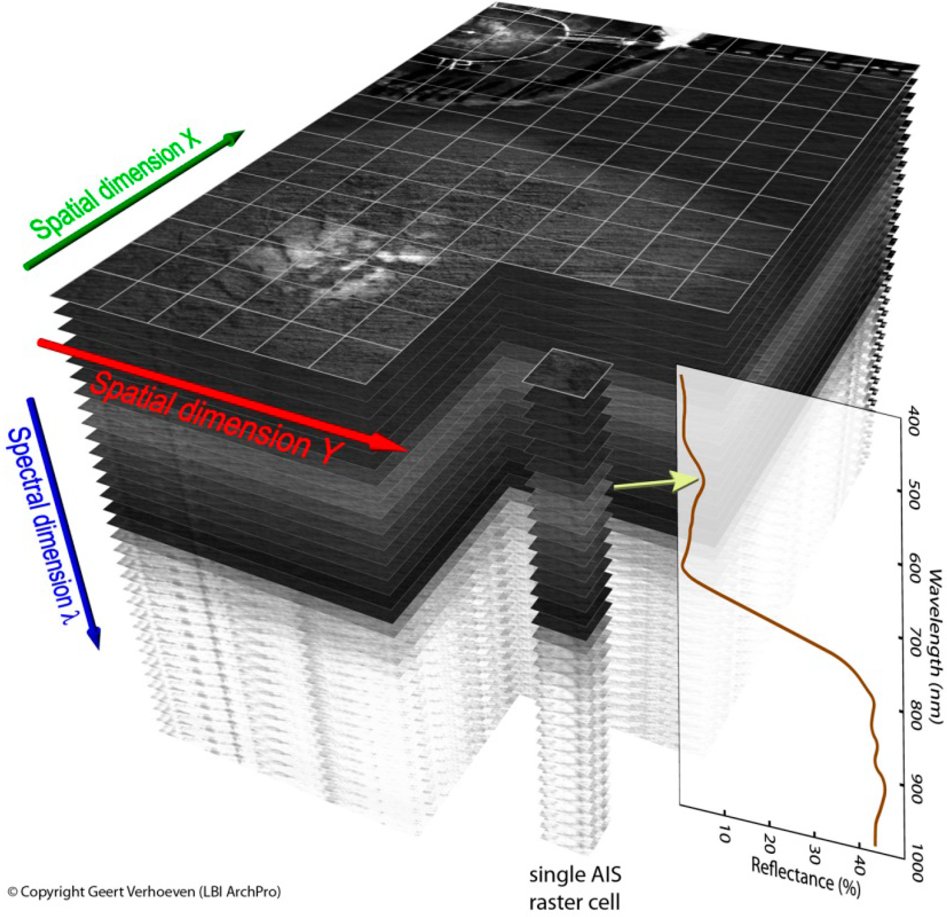
The resulting co-registered stack of image bands produced by IS can be considered a three-dimensional data cube (x, y, λ) in which the first two are the spatial dimensions, whereas the third axis contains the spectral dimension (i.e., those tens to hundreds of spectrally contiguous bands–Figure 1). This allows retrieving the spectral signature for individual objects, as well as the detection of subtle absorption features [24] (Table 1).
In archaeology, AIS is considered to have a huge potential for airborne prospection, because it is assumed to overcome the deficits of conventional and multispectral imagery and enhance the visibility of soil color differences and plant stress. Several studies have demonstrated the advantage of this imaging technique (e.g., [25–35]).
However, to fully exploit the potential offered by imaging spectrometers, a number of inherent problems have to be addressed by the image analyst (such as the large number of bands exhibiting high data redundancy and the low signal to noise ratio–see below), whereas, also, the most fruitful ways to visualize the data for a specific scientific investigation have to be explored. For research in archaeological prospection, suitable software solutions are needed, which can address these issues and let the user focus on a workflow to enhance the visibility of soil spectral differences and plant stress.
The objective of the present contribution is to introduce a toolbox (ARCTIS–ARChaeological Toolbox for Imaging Spectroscopy) programmed in MATLAB® (under Windows) and addressing the mentioned requests. Based on an explication of the potential and need of an AIS approach for archaeology, requirements for an archaeological analysis of AIS data are defined in Section 2. The general concept and important features are outlined in Section 3 using an exemplary AIS data set (Carnuntum; Austria) with 105 bands and 0.4 m ground sampling distance (GSD). After a discussion (Section 4), conclusions and a short outlook are provided in Section 5.
2. Requirements for Proper (Archaeological) Analysis of Imaging Spectroscopy Datasets
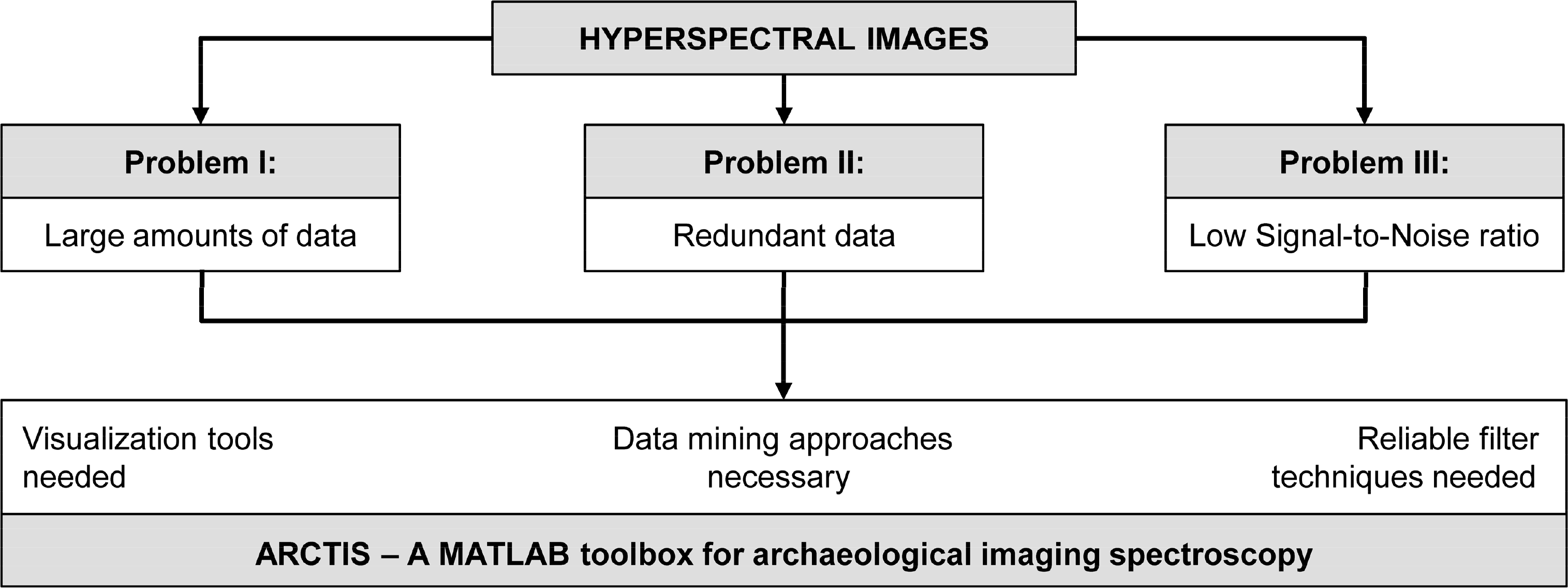
Compared to traditional MS image analysis, the inspection, visualization, and analysis of hyperspectral data sets from IS poses a number of challenges for which suitable software solutions are needed. Although a few commercial (e.g., Exelis ENVI) and free tools (e.g., Opticks) exists, there is currently no available free or low-cost software specialized in analyzing hyperspectral datasets for archaeological research. Archaeologists are, therefore, forced to build workarounds into existing (commercial) software packages (e.g., [25]). The main problems for efficiently using IS in archaeology relate to (Figure 2):
- (1)
The large number of spectral bands which need to be inspected;
- (2)
The inherent data redundancy in hyperspectral data sets;
- (3)
The relatively low signal-to-noise-ratio of the imagery, especially when utilizing sensors whose detector elements have a very small instantaneous field of view (IFOV) so that ground-sampling distances smaller than 1 meter can be obtained;
- (4)
Available software packages do not provide tools specifically aiding data reduction for archaeological feature detection (e.g., red-edge detection and parameterization).
In most cases, for example, it is not known beforehand in which spectral bands possibly present vegetation or soil marks will manifest themselves. Hence, the user has to interactively visualize a large number of spectral bands (and/or first-order derivatives) to decide where most information is present. This approach is different from most uses of hyperspectral imagery in which quantifiable parameters (such as chlorophyll content or soil organic carbon (SOC)) need to be obtained. Archaeologists are usually not interested in these bio-physical vegetation and soil parameters [36]. What matters are reliable, generally applicable methods that can be extended across entire landscapes, at different times of the day, and during various growing seasons, rather than very specific approaches that might vary from field to field, crop to crop, and by time of year. These methods should display the contrast exhibited (directly or indirectly) by an archaeological residue in its surrounding matrix, without the need to optimize the approach on the basis of vegetation species [37].
Valuable software should therefore help the analyst to choose a suitable band combination, for example through identification of information-rich layers. As edges and textural features may or may not be present in different spectral bands, calculations need to be performed easily amongst and across all available bands. While visually inspecting the data, the contrast setting parameters should be easily set so to highlight the (subtle) features the analyst is looking for. Stretch parameters should automatically adapt to the current cursor position and change when the cursor moves across the image.
Regarding data redundancy, the software should not only permit the application of data compression techniques (e.g., Principle Component Analysis or PCA), but, likewise, allow the derivation of the transformation matrix within small ‘training areas’ with known vegetation marks. Applying such data transformation to larger areas will possibly highlight the features sought after. Data compression techniques should also be implemented for combining data from different mapping devices (e.g., optical and geophysical sensors).
Hyperspectral datasets offer–despite data redundancy–rich information. Any software should assist in retrieving and visualizing this information. This includes for example the possibility to choose among a large set of vegetation indices (VI) with different functional forms [38]. To select appropriate spectral bands for a given functional form a suitable software solution should offer some assistance. In addition to two or three-band based VIs, spectral shapes should be described as detailed as possible, as this information is only accessible from IS and is usually rich in information [39]. Suitable techniques include for example the detection and parameterization of inflection points in the red-edge [40,41], as well as along the shoulders of other absorption bands for example related to water [42] or proteins [43].
Before starting the previously mentioned calculations, the software should, however, permit the user to eliminate/reduce sensor artifacts and noise stemming from the relatively low signal-to-noise ratio (SNR) of current imaging spectrometers. A suitable smoother should balance fidelity to the data and the roughness of the smoothed curve, while being easy to parameterize [44]. Importantly, the filter outcome should preserve the shape information of the observed spectral signature while minimizing edge effects and being fast. For optimum retrieval of the REIP (Red Edge Inflection Point) and other shape indicators, oversampling is beneficial [45,46].
Besides working along the z-axis (i.e., in direction of the wavelength range), a suitable filter should also be able to spatially (in x and y-direction) smooth/interpolate data. This is, for example, required when line dropouts occur and/or if point sampled (geophysical) data are to be integrated into the optical IS dataset.
To address the above mentioned problems and requests, ARCTIS was developed in cooperation between the Department of Prehistoric and Historical Archaeology of the University of Vienna and Vienna’s University of Natural Resources (BOKU). The toolbox is intended to highlight possibly occurring archaeological visibility marks (of which crop/vegetation marks are the most abundant) in hyperspectral datasets.
3. ARCTIS Toolbox Description
In the following, the toolbox will be introduced using an AIS survey of the Roman town of Carnuntum, which is a case study of the LBI ArchPro [47]. The area is located approximately 40 km south-east of Vienna on the southern bank of the Danube river (48°6′41′N, 16°51′57″E—WGS84). Data acquisition took place on the 5 June 2010, around 10:30 a.m., local time, in six parallel strips. The data were captured with a GSD of 40 cm in 105 spectral bands between 400 nm to 1000 nm and digitized as 12-bit integer Digital Numbers (DNs) (Table 2). After the necessary georeferencing of the individual flight strips (executed in ReSe Application PARGE), the data were ready to import in ARCTIS.
3.1. Overall Philosophy and Design of ARCTIS
ARCTIS is a user-friendly MATLAB® toolbox with a corresponding graphical user interface (GUI) that helps the image analyst–not necessarily a specialist in remote sensing or in imaging spectroscopy—to maximize the information extracted from the recorded 3D data cube. It is a tool to display hyperspectral data (multilayer TIFF images or ENVI files) in many different ways, and to retrieve as many pieces of information as possible from the imagery. As such, it was created to test currently available AIS processing practices, as well as validate the value of completely new information extraction techniques.
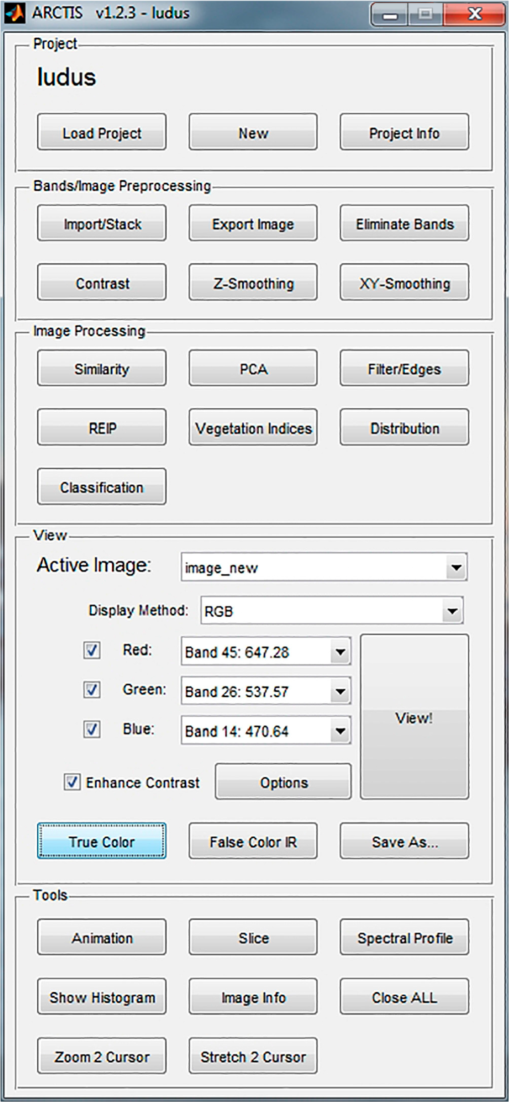
The GUI is divided into five sections (Figure 3), which follow a hypothetical workflow:
- ➢
Section 1: Project management.
- ➢
Section 2: Image pre-processing, including image import/export, data stacking, the elimination of specific bands, functions for contrast adjustment and smoothing in z-, as well as xy-, directions.
- ➢
Section 3: Image processing functions, grouped into similarity index calculation, principal component analysis, low/high pass filters and edge detection functions, inflection point calculation (see below), vegetation index calculation, distribution fitting (see below), and (k-means) data clustering.
- ➢
Section 4: Display control, visualization and output.
- ➢
Section 5: Contains several tools, which are helpful for image analysis, such as displaying an animated sequence of the 3D data cube, viewing data along slices, and displaying spectral profiles of selected pixels.
As it was created to test currently available AIS processing practices, the toolbox offers a variety of different image processing algorithms. To help the image analyst to remember all individual processing steps, all functions (and their parameters) that are applied to each file are logged into a history file. History files are simple ASCII text files, which have the same name as the image file and are located in the same folder. As each image processing function results in a new image with a new file name, ARCTIS takes all the history information out of the original file and includes it in the file of the new image. In this way, all functions and parameters that produced a given image are included in its history file. Hence, all results can be re-created if necessary.
3.2. Enhanced Data Processing
The following section will describe features, which are considered important for the archaeologist. They are often not available in commercial software products and can be regarded as an important enhancement of the toolbox.
3.2.1. Data Smoothing along the Spectral Dimension (z-Direction)
Imagery derived from imaging spectroscopy has often a relatively low SNR. Therefore it is strongly recommended to apply a suitable filter/smoother to the 3D data cube before any other processing step [48–51]. In this way, the useful signal is kept while most noise is eliminated. Although time demanding, data smoothing enhances the quality of all subsequent analysis processes.
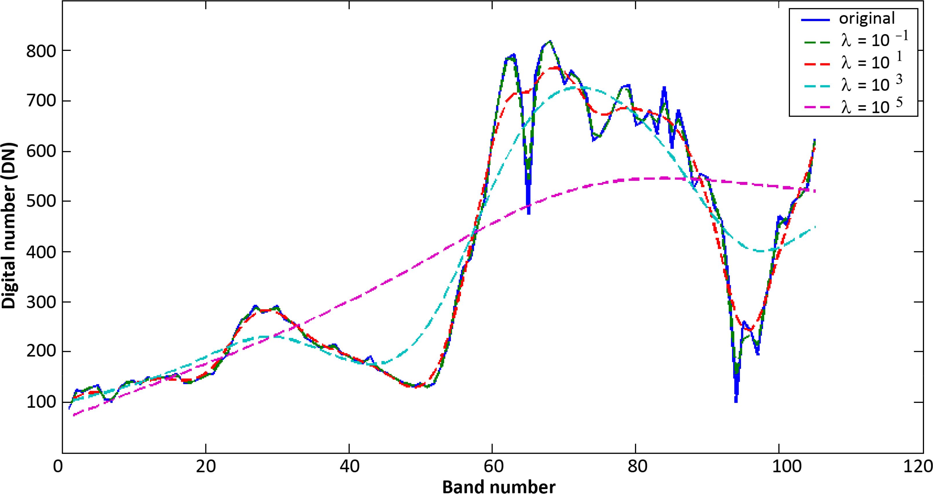
The smoothing algorithm used in ARCTIS was originally developed by Whittaker [52] and later modified and implemented in MATLAB® by Paul Eilers [44]. The “Whittaker smoother” is based on penalized least squares. It fits a discrete series to discrete data and penalizes the roughness of the smooth curve. In this way, it balances reliability of the data (ρλ) and roughness of the fitted data (ρ*λ). The smoother the result, the more it will deviate from the input data. A balanced combination of the two goals is the sum (Q):
The lack of fit to the data S is measured as the usual sum of squares of differences. The roughness of the smoothed curve R is expressed here as third order differences. The smoothing parameter λ is chosen by the user (trial-and-error). The aim of penalized least squares is to find the series that minimizes Q. The larger the parameter λ, the greater is the influence of R on the goal Q and the smoother will be the curve (at the cost of the degradation of the fit). For a detailed mathematical background of the Whittaker smoother, please refer to the mentioned original documents, as well as Atzberger and Eilers [53] and Atkinson et al. [54]. The latter two references apply the Whittaker smoother in the temporal domain.
In ARCTIS, each AIS pixel is smoothed independently along the z-axis (i.e., spectral dimension) leading to smoothed spectral profiles. For every pixel location, all layer values are taken and smoothed values are calculated and written into a new image. The smoother treats all bands as if they were equally spaced in the wavelength range. The number of input bands equals the number of output bands (see below for oversampling data using the Whittaker smoother). The roughness of the resulting curve is hereby solely defined by the so-called smoothing parameter lambda (λ), where the user is free to select the data point (pixel) displayed for “optimization” of λ.
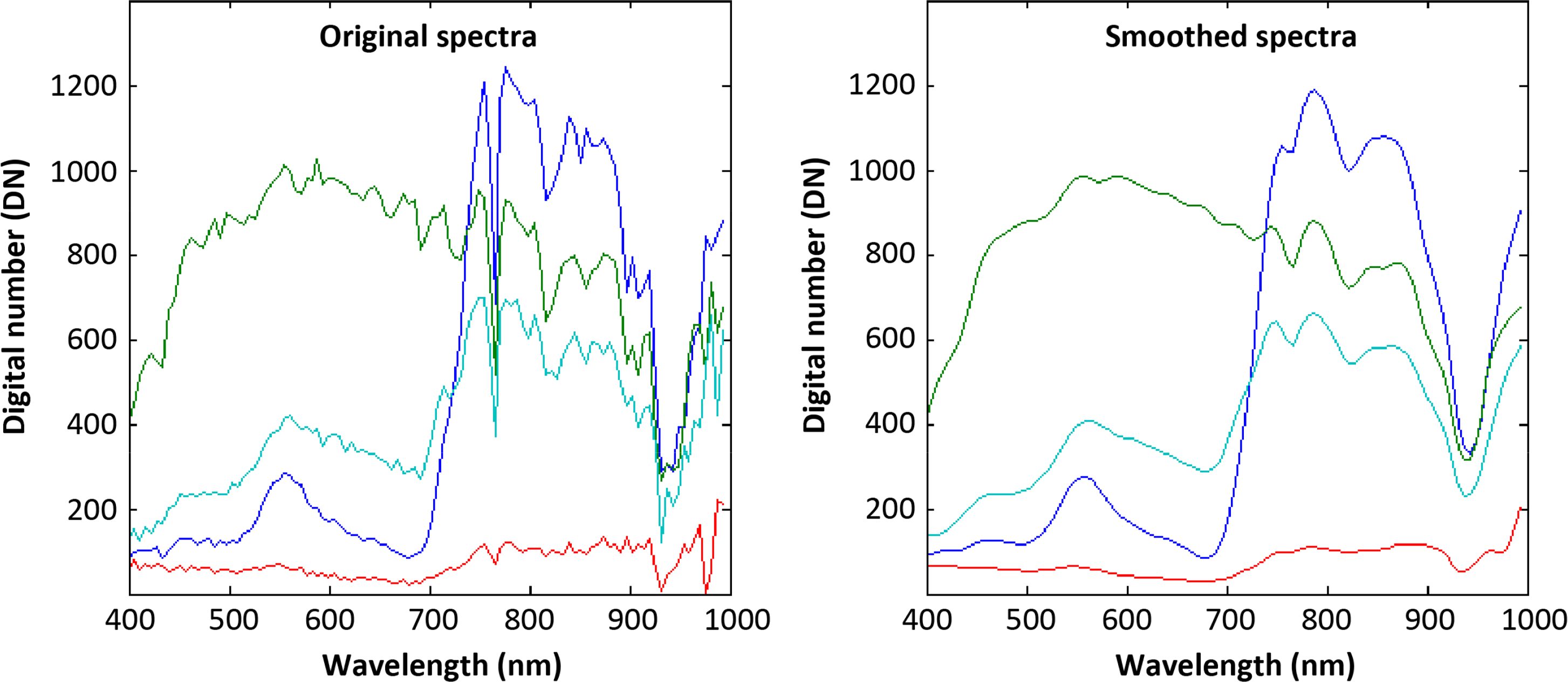
The effect of selecting different smoothing parameters on a noisy spectral signature is shown in Figure 4; the smaller the smoothing parameter the better are the original values fitted. However, at the same time, the resulting curve is rough with (too) many inflection points not referring to any known absorption feature. Example profiles before and after smoothing (with λ = 10) are shown in Figure 5. The value of λ = 10 was chosen after some trial-and-error. It can be seen that most of the noise in the data can be removed (e.g., data spikes). At the same time, the shape of the reflectance curve is well preserved.
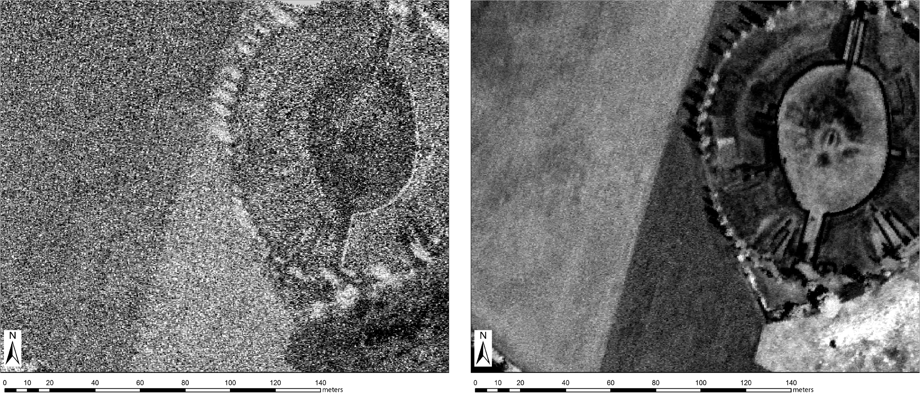
The (positive) effect of applying the Whittaker smoother is further illustrated in Figure 6 by showing the first derivative of the hyperspectral data cube for the green waveband around 540 nm. Whereas the first derivative shows a very noisy pattern when calculated from the original data (left), the same image looks much clearer if the data were smoothed before display (right).
3.2.2. Shape Descriptors: Inflection Points and Spectral Shifts
A number of studies have demonstrated the added value of detecting inflection points in the spectral shapes of vegetated pixels [55–59]. Different methods were designed to extract the desired wavelength position [40,60]. The theoretical analysis of [61] demonstrated that detecting inflection points (and, thus, spectral shifts) in vegetation spectra reduce the negative impacts of variations in soil brightness, irradiance conditions and atmospheric perturbations. Despite this long-lasting knowledge about the prospects of this indicator, currently, no commercial software has implemented suitable algorithms.
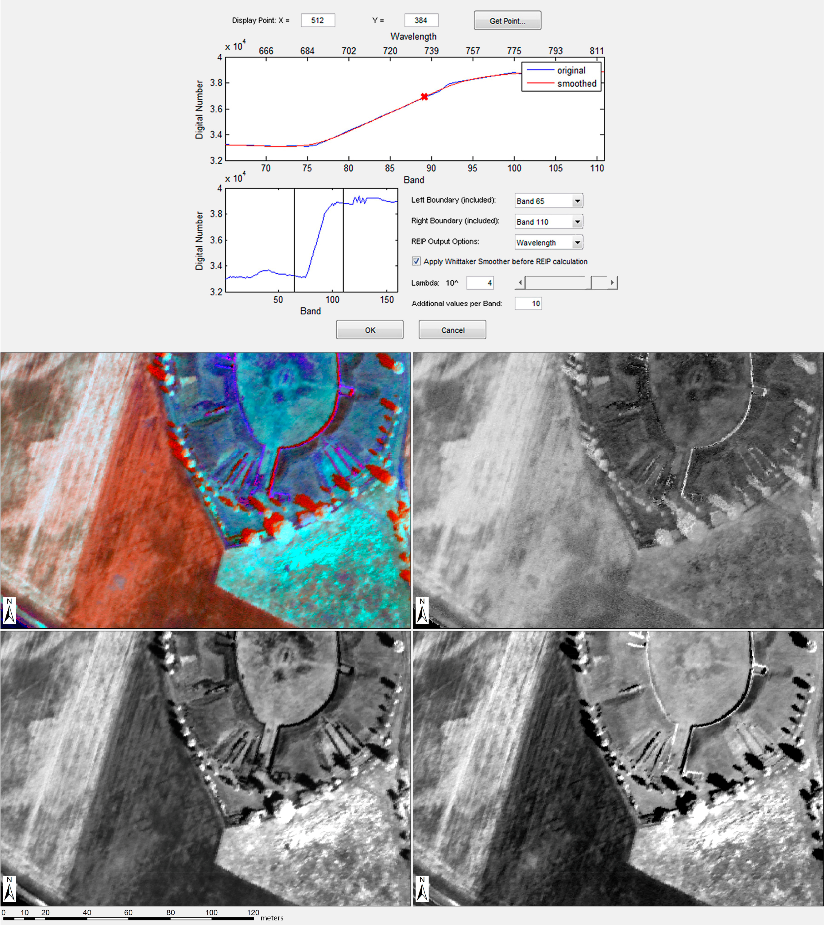
In ARCTIS, inflection points are included which identify for each pixel the location (in terms of band number) of the highest (absolute) gradient in the spectral profile (marked by the bold red “x” in Figure 7). In addition to this “inflection point” (first output layer), the algorithm also outputs two additional indicators linked to this point: the value of the gradient itself (second output), and the level of reflectance for the wavelength of maximum gradient (third output) (the three gray-level images in Figure 7 illustrate these outputs). Together, the three indicators were found very informative for archaeological research [62].
The search for the maximum derivate can be restricted in ARCTIS to a specific spectral range. In Figure 7(top), the restriction is set between bands 50 and 62 (corresponding to a spectral range of 676–746 nm); the edges are indicated by vertical lines in the lower part of the figure. Confining the algorithm to this so-called “red-edge” band will yield the “red edge inflection point” (REIP). The red edge is the steep increase of the reflectance curve between 690 nm and 750 nm where the chlorophyll absorption vanishes and the reflectance increases towards the NIR plateau. In this wavelength range, the REIP is directly proportional to the total canopy chlorophyll content [61]. However, it is also possible (and recommended) to analyze other absorption features, as, for example, around the green peak, or in vicinity to water absorption or protein bands [8].
Note that the standard calculation of REIP always yields inflection points being integers (e.g., one of the available bands). To get more accurate results (i.e., floating values), ARCTIS allows the user to first interpolate/oversample the original data by applying a Whittaker smoother to create a large number of fictional “bands” between the original data values before identifying the maximum of the first derivative. The positive effect of smoothing and smoothing/oversampling is illustrated in Figure 8. Clearly, more details can be seen when the REIP is calculated from smoothed data (Figure 8c) compared to the original data (Figure 8b). Even more details become visible when the oversampling procedure is applied before calculating of REIP. Two inflection point images calculated outside the red edge region are displayed in Figure 9 for comparison.
3.2.3. Distribution Fitting
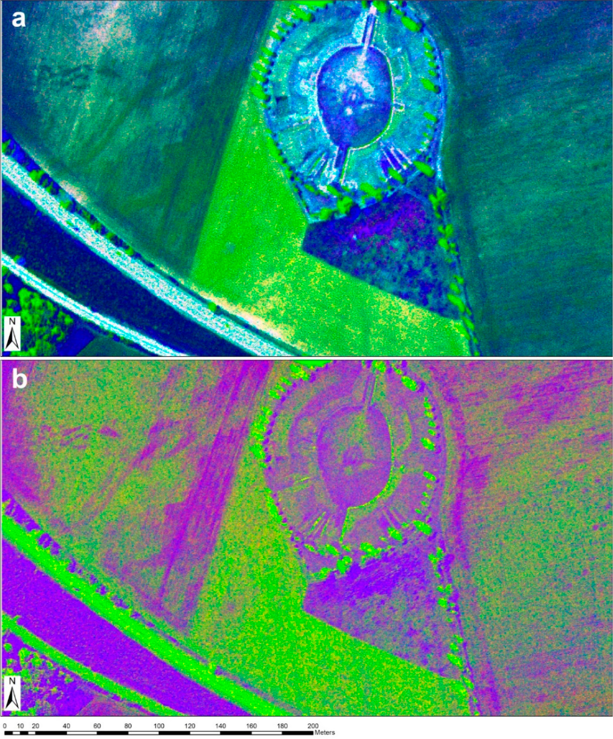
Usually, in remote sensing the bands in a (hyper-) spectral dataset are interpreted in their “natural order” following increasing wavelength. However, it is also possible to ignore wavelength information. In such a case, one associates to each pixel a vector of n values (from n spectral bands). If all the values from the vector are ordered by increasing value, they form a histogram (Figure 10). In the presented approach, a histogram is thus computed from all DNs describing one hyperspectral pixel (i.e., the complete spectral signature of that raster cell). This histogram can be considered a graphical representation of an empirical distribution [63]. Afterwards, a user-defined theoretical probability density function (PDF) is fitted to this histogram to mathematically describe this specific empirical distribution. Thus, a histogram is formed from the acquired signal (i.e., the pixel’s DNs) and the PDF is the corresponding curve that characterizes the distribution of the underlying process or population [64]. In ARCTIS, a number of discrete and continuous theoretical PDFs reside (although mathematicians would use the term Probability Mass Function (PMF) for discrete random variables [64]). Any of these PDFs is defined by one or more parameters. The normal PDF describing the normal distribution, for instance, is parameterized in terms of a mean parameter μ and a standard deviation σ [65]. All ARCTIS PDFs, parameterized by one to three parameters (Table 3), can be fitted (pixel-by-pixel) to the pixel-specific histograms. After fitting the selected PDF, the resulting parameter fields can be visualized as an image. The first promising results were obtained using this new technique by Verhoeven et al. [62].
Exemplary results are shown in Figure 11 illustrating the potential of this kind of data analysis. It has to be noted, however, that for some distributions, the fitting process uses an iterative algorithm. Hence, deriving these images can be quite time-consuming. To the author’s knowledge, no other software exists that currently offers this interesting feature. For a more elaborate discussion of this feature’s archaeological potential, consider [66].
3.3. Visualization Tools
As the main idea of the toolbox is to provide an easy to use means for exploring an AIS dataset, some visualization tools seemed to be necessary that would help the user to mine their hyperspectral data and identify spectral bands useful for best discriminating soil and vegetation marks.
As a standard tool, the reflectance curves of user-selected pixels can be displayed. More importantly, the entire image cube can be visualized along user-selected vertical or horizontal slices (Figure 12). A horizontal slice, for example, corresponds to all data (in column and layer direction) along a fixed row number. If located above a known soil or vegetation mark, this permits the user to detect band numbers (wavelengths) where these marks have maximum contrast to the surrounding matrix.
The human visual system is known to be very effective in recognizing structures and movements [67]. A number of animated visualization tools have therefore been added permitting to display the layers of the active image sequentially (and repeatedly) with a user-specified frequency (speed; in Hertz). As IS datasets store much information in local derivatives (i.e., along the wavelength axis), the user cannot only display animations of the original data (standard setting), but also first derivatives calculated on-the-fly in either original (signed) or absolute values (unsigned). Moreover, it is possible to display triplets of adjacent bands as RGB either in non-overlapping or overlapping mode. This latter option gives some information about the shape of the spectral signatures. All animations can be visualized in different colormaps and exported as animated GIF (Graphics Interchange Format), uncompressed AVI (Audio Video Interleave) movie file or lossless Motion JPEG 2000 compressed *.mj2 files.
4. Discussion
The main aim of this specific AIS toolbox (called ARCTIS) is to enable users to inspect, visualize and analyze hyperspectral data sets. Therefore, the toolbox includes a wide variety of tools to test currently available IS processing practices, as well as validate the value of completely new information extraction techniques. The starting point for its development was the need to collect and compile tools, which are especially useful for archaeologists who want to identify crop and soil marks from airborne IS data.
It was, therefore, necessary to adapt the software to the archaeologist’s needs. First of all, a GUI had to be designed that would even allow a non-specialist in remote sensing to apply ARCTIS in a straightforward way. Based on the authors’ conviction that only high spatial resolution datasets (GSD < 1 m) will be useful for archaeological prospection, the toolbox includes a Whittaker smoother to reduce the inherent sensor artifacts and noise while preserving the shape information of the observed spectral signature. Other needs are the assistance to identify information-rich layers, which is realized through tools for interactive visualization of the usually large number of spectral bands, and the application of data compression techniques (e.g., PCA), based on selected sample areas with known vegetation marks. New tools, which are otherwise not available in commercial IS software, are the calculation of inflection points in the red-edge and along the shoulders of other absorption bands as well as novel distribution fittings. They can yield new insights into crop vigor and crop stress. Their archaeological potential will investigated more thoroughly in a forthcoming paper [66].
The concept of history files is of high importance to assist testing and developing one’s own workflow for AIS processing. This allows the retrieving of all functions and their parameters, which have produced a specific output. In this way, processing of IS data becomes transparent and repeatable, which is a necessity for scientific use. This is even more important given the fact that the toolbox offers a variety of different image processing algorithms which can be consecutively arranged in a process chain.
These requirements, however, also resulted in restrictions. More than anything else, this toolbox and its residing algorithms must be considered a proto-typing and testing environment. It is well known that the high-level MATLAB® programming language focuses more on the ease of code development than on the performance often found in low-level languages such as C/C++ and Fortran. This characteristic becomes very apparent when executing the distribution fitting approach. Since all operations are executed on a pixel-by-pixel basis, the whole operation becomes very time-consuming in a MATLAB®-driven environment, which in turn restrains it from numerous test runs on large datasets. Although ARCTIS was initially developed to mine archaeological AIS data cubes, it is—at this stage—not the ideal tool for processing large datasets.
Therefore, this toolbox is currently used to tile large hyperspectral scenes during import and work on these individual tiles afterwards. Using these tiles, the currently embedded algorithms can be validated, while new processing methods can be proto-typed and still be called from the easy-to-use GUI. In the near future, when several AIS datasets have been processed and the outcome of specific processing workflows was validated by different practitioners, those specific algorithms (or combinations of them) that proved most useful will be implemented in C or C++ for faster execution, while the MATLAB® GUI can still be used to call these external programs.
Initially, ARCTIS was developed to purely serve academic archaeological purposes. Given the fact that many of its residing processing and visualization tools cannot be found elsewhere and commercial software is often costly and less straightforward to use, the authors decided to make the toolbox and its source code freely available under creative commons license for all interested parties (via download from http://luftbildarchiv.univie.ac.at). Together with some test datasets, this open access will enable interested students and remote sensing professionals to become acquainted with AIS, while other scientists can contribute with new algorithms to further expand and even optimize ARCTIS.
5. Conclusions
By programming ARCTIS as a specific airborne imaging spectroscopy (AIS) toolbox for archaeological purposes, a tool was created to test currently available AIS processing practices as well as validate the value of completely new information extraction techniques. The ARCTIS toolbox is programmed in MATLAB® (under Windows) and comes with a user-friendly graphical user interface (GUI). The GUI is conceived in such a way that also non-experts in remote sensing can retrieve useful information from this relatively new-but valuable-data source.
Compared to commercial software products, a number of features are found in this toolbox that permit an enhanced data processing and visualization. In particular, the Whittaker-based smoother, with its over-sampling capacity, permits to get rid of sensor noise while allowing the parameterization of curve features such as the red-edge inflection point (REIP) with unprecedented accuracy. Additional functionality is provided to permit further access to the spectral shape information offered by imaging spectroscopy. Interesting results can also be obtained from fitting probability density functions to the pixel-based histograms followed by a visualization of the fitted model parameters. A number of visualization tools further help the image analyst to detect subtle visibility marks. We therefore expect that this toolbox will be of great benefit in archaeological research, as well as in other disciplines dealing with hyperspectral datasets. The toolbox and its source code will be made available to interested researchers via download ( http://luftbildarchiv.univie.ac.at)—with need to reference to the current publication.
Acknowledgments
We gratefully acknowledge those people having made available their MATLAB® codes so that we could integrate the proposed functionalities into ARCTIS: P.H.C. Eilers for the MATLAB®-based implementation of the Whittaker smoother, D. Garcia for the two-dimensional smoothing and gap-filling algorithm, and B. Shoelsen for his zoom2cursor function which inspired the Stretch2Cursor and Zoom2Cursor functionality of ARCTIS. We also would like to thank F. Totir, J. Tuszynski and I. Howat for making their ENVI read/write scripts available on the MATLAB® File Exchange platform. Their work helped to overcome difficulties in handling ENVI files. We thank the independent reviewers for their useful comments.
Author Contributions
Clement Atzberger, Michael Doneus and Geert Verhoeven designed the needs leading to the ARCTIS software tool, which itself was programmed in Matlab by Clement Atzberger and Michael Wess. The paper was conceived and written by Clement Atzberger, Michael Doneus and Geert Verhoeven. Figures and illustrations were provided by Geert Verhoeven, Michael Doneus and Clement Atzberger.
Conflicts of Interest
The authors declare no conflict of interest.
References
- Verhoeven, G. Providing an archaeological bird’s-eye view: An overall picture of ground-based means to execute low-altitude aerial photography (LAAP) in Archaeology. Archaeol. Prospect 2009, 16, 233–249. [Google Scholar]
- Carter, G.A. Responses of leaf spectral reflectance to plant stress. Am. J. Bot 1993, 80, 239–243. [Google Scholar]
- Carter, G.A.; Rebbeck, J.; Percy, K. Leaf optical properties in Liriodendron tulipifera and Pinus strobus as influenced by increased atmospheric ozone and carbon dioxide. Can. J. For. Res 1995, 25, 407–412. [Google Scholar]
- Hendry, G.A.; Houghton, J.D.; Brown, S.B. Tansley review no. 11. The degradation of chorophyll—A biological enigma. New Phytol 1987, 107, 255–302. [Google Scholar]
- Knipling, E.B. Physical and physiological basis for the reflectance of visible and near-infrared radiation from vegetation. Remote Sens. Environ 1970, 1, 155–159. [Google Scholar]
- Peñuelas, J.; Filella, I. Visible and near-infrared reflectance techniques for diagnosing plant physiological status. Trends Plant Sci 1998, 3, 151–156. [Google Scholar]
- Carter, G.A. General spectral characteristics of leaf reflectance responses to plant stress and implications for the remote sensing of vegetation. Proceedings of the 2001 ASPRS Annual Conference: Gateway to the New Millennium, St. Louis, MO, USA, 23–27 April 2001.
- Adams, M.L.; Philpot, W.D.; Norvell, W.A. Yellowness index: An application of spectral second derivatives to estimate chlorosis of leaves in stressed vegetation. Int. J. Remote Sens 1999, 20, 3663–3675. [Google Scholar]
- Merzlyak, M.N.; Gitelson, A.A. Why and what for the leaves are yellow in Autumn? On the interpretation of optical spectra of senescing leaves (Acerplatanoides L.). J. Plant Physiol 1995, 145, 315–320. [Google Scholar]
- Young, A.; Britton, G. Carotenoids and stress. In Stress Responses in Plants; Alscher, R.G., Cumming, J.R., Eds.; Wiley-Liss: New York, NY, USA, 1990; pp. 87–112. [Google Scholar]
- Goetz, A.F. Three decades of hyperspectral remote sensing of the Earth: A personal view. Remote Sens. Environ 2009, 113, S5–S16. [Google Scholar]
- Schaepman, M.E.; Ustin, S.L.; Plaza, A.J.; Painter, T.H.; Verrelst, J.; Liang, S. Earth system science related imaging spectroscopy—An assessment. Remote Sens. Environ 2009, 113, 123–137. [Google Scholar]
- Ustin, S.L.; Roberts, D.A.; Gamon, J.A.; Asner, G.P.; Green, R.O. Using imaging spectroscopy to study ecosystem processes and properties. BioScience 2004, 54, 523–534. [Google Scholar]
- Borengasser, M.; Hungate, W.S.; Watkins, R.L. Hyperspectral Remote Sensing: Principles and Applications (Remote Sensing Applications Series); CRC Press: Boca Raton, FL, USA, 2008; p. 119. [Google Scholar]
- Berger, M.; Rast, M.; Wursteisen, P.; Attema, E.; Moreno, J.; Müller, A.A.; Beisl, U.; Richter, R.; Schaepman, M.E.; Strub, G.; et al. The DAISEX campaigns in support of a future land-surface-processes mission. ESA Bull 2001, 105, 101–111. [Google Scholar]
- Cocks, T.; Jenssen, R.; Stewart, A.; Wilson, I.; Shields, T. The HyMapTM airborne hyperspectral sensor: The system, calibration and performance. Proceedings of the 1st EARSEL Workshop on Imaging Spectroscopy, Zürich, Swiss, 6–8 October 1998.
- Green, R.O.; Eastwood, M.L.; Sarture, C.M.; Chrien, T.G.; Aronsson, M.; Chippendale, B.J.; Faust, J.A.; Pavri, B.E.; Chovit, C.J.; Solis, M.; et al. Imaging spectroscopy and the Airborne Visible/Infrared Imaging Spectrometer (AVIRIS). Remote Sens. Environ 1998, 65, 227–248. [Google Scholar]
- Holzwarth, S.; Müller, A.; Habermeyer, M.; Richter, R.; Hausold, A.; Thiemann, S.; Strobl, P. HySens-DAIS/ROSIS imaging spectrometers at DLR. Proceedings of the 3rd EARSeL Workshop on Imaging Spectroscopy, Herrsching, Germany, 13–16 May 2003.
- Müller, A.A.; Hausold, A.; Strobl, P.; Ehlers, M. HySens-DAIS/ROSIS imaging spectrometers at DLR. Proc. SPIE 2001, 4545. [Google Scholar] [CrossRef]
- Vane, G.; Green, R.O.; Chrien, T.G.; Enmark, H.T.; Hansen, E.G.; Porter, W.M. The Airborne Visible/Infrared Imaging Spectrometer (AVIRIS). Remote Sens. Environ 1993, 44, 127–143. [Google Scholar]
- Pearlman, J.S.; Barry, P.S.; Segal, C.C.; Shepanski, J.; Beiso, D.; Carman, S.L. Hyperion, a space-based imaging spectrometer. IEEE Trans. Geosci. Remote Sens 2003, 41, 1160–1173. [Google Scholar]
- Kaufmann, H.; Segl, K.; Chabrillat, S.; Hofer, S.; Stuffler, T.; Müller, A.A.; Richter, R.; Schreier, G.; Haydn, R.; Bach, H. EnMAP—A hyperspectral sensor for environmental mapping and analysis. Proceedings of the 2006 IEEE International Geoscience and Remote Sensing Symposium, Denver, CO, USA, 31 July–4 August 2006; pp. 1617–1619.
- Kaufmann, H.; Förster, S.; Wulf, H.; Segl, K.; Guanter, L.; Bochow, M.; Heiden, U.; Müller, A.; Heldens, W.; Schneiderhan, T.; et al. Science Plan of the Environmental Mapping and Analyis Program (EnMAP): Scientific Technical Report. Available online: http://www.enmap.org/sites/default/files/pdf/pub/121026_EnMAP_SciencePlan_dpi150.pdf (accessed on 6 March 2014).
- Hyperspectral Remote Sensing of Vegetation; Thenkabail, P.S., Lyon, J.G., Huete, A.R., Eds.; CRC Press: Boca Raton, FL, USA, 2012; p. 705.
- Aqdus, S.A.; Hanson, W.S.; Drummond, J. The potential of hyperspectral and multi-spectral imagery to enhance archaeological cropmark detection: A comparative study. J. Archaeol. Sci 2012, 39, 1915–1924. [Google Scholar]
- Bassani, C.; Cavalli, R.M.; Goffredo, R.; Palombo, A.; Pascucci, S.; Pignatti, S. Specific spectral bands for different land cover contexts to improve the efficiency of remote sensing archaeological prospection: The Arpi case study. J. Cult. Herit 2009, 10, e41–e48. [Google Scholar]
- Bennett, R.; Welham, K.; Hill, R.A.; Ford, A.L.J. The application of vegetation indices for the prospection of archaeological features in grass-dominated environments. Archaeol. Prospect 2012, 19, 209–218. [Google Scholar]
- Cavalli, R.M.; Colosi, F.; Palombo, A.; Pignatti, S.; Poscolieri, M. Remote hyperspectral imagery as a support to archaeological prospection. J. Cult. Herit 2007, 8, 272–283. [Google Scholar]
- Forte, E.; Pipan, M.; Sugan, M. Integrated geophysical study of archaeological sites in the Aquileia Area. Proceedings of the 1st Workshop on the New Technologies for Aquileia (NTA-2011), Aquileia, Italy, 2 May 2011.
- Merola, P. Tecniche di telerilevamento iperspettrale applicate alla ricerca archeologica. Il caso di Lilybaeum. Archeologia Aerea. Studi Aerotopografia Archeol 2005, 1, 301–317. [Google Scholar]
- Pascucci, S.; Cavalli, R.M.; Palombo, A.; Pignatti, S. Suitability of CASI and ATM airborne remote sensing data for archaeological subsurface structure detection under different land cover: The Arpi case study (Italy). J. Geophys. Eng 2010, 7, 183–189. [Google Scholar]
- Savage, S.H.; Levy, T.E.; Jones, I.W. Prospects and problems in the use of hyperspectral imagery for archaeological remote sensing: A case study from the Faynan copper mining district, Jordan. J. Archaeol. Sci 2012, 39, 407–420. [Google Scholar]
- Traviglia, A. A semi-empirical index for estimating soil moisture from MIVIS data to identify subsurface archaeological sites. Proceedings of the Atti della 9a Conferenza Nazionale ASITA, Catania, Italy, 15–18 November 2005; pp. 1969–1974.
- Traviglia, A. Archaeological usability of hyperspectral images: Successes and failures of image processing techniques. Proceedings of the 2nd International Conference on Remote Sensing in Archaeology, CNR, Rome, Italy, 4–7 December 2006; pp. 123–130.
- Traviglia, A. MIVIS hyperspectral sensors for the detection and GIS supported interpretation of subsoil archaeological sites. Proceedings of the 34th Conference on Digital Discovery: Exploring New Frontiers in Human Heritage, CAA 2006, Computer Applications and Quantitative Methods in Archaeology, Fargo, ND, USA, 24–26 April 2006.
- Beck, A.R. Archaeological applications of multi/hyper-spectral data-Challenges and potential. In Remote Sensing for Archaeological Heritage Management, Proceedings of the 2011 11th EAC Heritage Management Symposium, Reykjavík, Iceland, 25–27 March 2010; pp. 87–97.
- Verhoeven, G. Beyond Conventional Boundaries: New Technologies, Methodologies, and Procedures for the Benefit of Aerial Archaeological Data Acquisition and Analysis. Ph.D. Thesis. Ghent University, Ghent, Belgium, 2009. [Google Scholar]
- Bannari, A.; Morin, D.; Bonn, F.; Huete, A.R. A review of vegetation indices. Remote Sens. Rev 1995, 13, 95–120. [Google Scholar]
- Thenkabail, P.S.; Enclona, E.A.; Ashton, M.S.; van der Meer, B. Accuracy assessments of hyperspectral waveband performance for vegetation analysis applications. Remote Sens. Environ 2004, 91, 354–376. [Google Scholar]
- Cho, M.A.; Skidmore, A.K.; Atzberger, C. Towards red-edge positions less sensitive to canopy biophysical parameters for leaf chlorophyll estimation using properties optique spectrales des feuilles (PROSPECT) and scattering by arbitrarily inclined leaves (SAILH) simulated data. Int. J. Remote Sens 2008, 29, 2241–2255. [Google Scholar]
- Vogelmann, J.E.; Rock, B.N.; Moss, D.M. Red edge spectral measurements from sugar maple leaves. Int. J. Remote Sens 1993, 14, 1563–1575. [Google Scholar]
- Gao, B.-C. NDWI—A normalized difference water index for remote sensing of vegetation liquid water from space. Remote Sens. Environ 1996, 58, 257–266. [Google Scholar]
- Kokaly, R.F. Investigating a physical basis for spectroscopic estimates of leaf nitrogen concentration. Remote Sens. Environ 2001, 75, 153–161. [Google Scholar]
- Eilers, P.H.C. A perfect smoother. Anal. Chem 2003, 75, 3631–3636. [Google Scholar]
- Clevers, J.G.P.W.; Kooistra, L.; Salas, E.A.L. Study of heavy metal contamination in river floodplains using the red-edge position in spectroscopic data. Int. J. Remote Sens 2004, 25, 3883–3895. [Google Scholar]
- Dawson, T.P. The potential for estimating chlorophyll content from a vegetation canopy using the Medium Resolution Imaging Spectrometer (MERIS). Int. J. Remote Sens 2000, 21, 2043–2051. [Google Scholar]
- Trinks, I.; Neubauer, W.; Doneus, M. Prospecting archaeological landscapes. Proceedings of the 4th International Conference on Progress in Cultural Heritage Preservation, EuroMed 2012, Lemessos, Cyprus, 29 October–3 November 2012; pp. 21–29.
- Curran, P.J.; Dungan, J.L.; Macler, B.A.; Plummer, S.E.; Peterson, D.L. Reflectance spectroscopy of fresh whole leaves for the estimation of chemical concentration. Remote Sens. Environ 1992, 39, 153–166. [Google Scholar]
- Ruffin, C.; King, R.L.; Younan, N.H. A combined derivative spectroscopy and savitzky-golay filtering method for the analysis of hyperspectral data. GISci. Remote Sens 2008, 45, 1–15. [Google Scholar]
- Shafri, H.Z.M.; Yusof, M.R.M. Trends and issues in noise reduction for hyperspectral vegetation reflectance spectra. Eur. J. Sci. Res 2009, 29, 404–410. [Google Scholar]
- Vaiphasa, C. Consideration of smoothing techniques for hyperspectral remote sensing. ISPRS J. Photogramm. Remote Sens 2006, 60, 91–99. [Google Scholar]
- Whittaker, E.T. On a new method of graduation. Proc. Edinb. Math. Soc 1923, 41, 63–75. [Google Scholar]
- Atzberger, C.; Eilers, P.H.C. Evaluating the effectiveness of smoothing algorithms in the absence of ground reference measurements. Int. J. Remote Sens 2011, 32, 3689–3709. [Google Scholar]
- Atkinson, P.M.; Jeganathan, C.; Dash, J.; Atzberger, C. Inter-Comparison of four models for smoothing satellite sensor time-series data to estimate vegetation phenology. Remote Sens. Environ 2012, 123, 400–417. [Google Scholar]
- Boochs, F.; Kupfer, G.; Dockter, K.; Kühbauch, W. Shape of the red edge as vitality indicator for plants. Int. J. Remote Sens 1990, 11, 1741–1753. [Google Scholar]
- Baret, F.; Champion, I.; Guyot, G.; Podaire, A. Monitoring wheat canopies with a high spectral resolution radiometer. Remote Sens. Environ 1987, 22, 367–378. [Google Scholar]
- Gitelson, A.A.; Merzlyak, M.N.; Lichtenthaler, H.K. Detection of red edge position and chlorophyll content by reflectance measurements near 700 nm. J. Plant Physiol 1996, 148, 501–508. [Google Scholar]
- Darvishzadeh, R. Hyperspectral Remote Sensing of Vegetation Parameters Using Statistical and Physical Models., Ph.D. Thesis. Wageningen, University, Wageningen, The Netherlands, 2008.
- Darvishzadeh, R.; Atzberger, C.; Skidmore, A.K.; Abkar, A.A. Leaf Area Index derivation from hyperspectral vegetation indices and the red edge position. Int. J. Remote Sens 2009, 30, 6199–6218. [Google Scholar]
- Gupta, R.K.; Vijayan, D.; Prasad, T.S. Comparative analysis of red-edge hyperspectral indices. Adv. Space Res 2003, 32, 2217–2222. [Google Scholar]
- Baret, F.; Jacquemoud, S.; Guyot, G.; Leprieur, C. Modeled analysis of the biophysical nature of spectral shifts and comparison with information content of broad bands. Remote Sens. Environ 1992, 41, 133–142. [Google Scholar]
- Verhoeven, G.; Doneus, M.; Atzberger, C.; Wess, M.; Ruš, M.; Pregesbauer, M.; Briese, C. New approaches for archaeological feature extraction of airborne imaging spectroscopy data. Proceedings of the 10th International Conference on Archaeological Prospection, Vienna, Austria, 29 May–2 June 2013; pp. 13–15.
- Trauth, M.H. MATLAB® Recipes for Earth Sciences, 3rd ed.; Springer: Berlin/Heidelberg, Germany, 2010; p. 336. [Google Scholar]
- Smith, S.W. The Scientist and Engineer’s Guide to Digital Signal Processing, 1st ed.; California Technical Publishing: San Diego, CA, USA, 1997; p. 626. [Google Scholar]
- Introduction to the Practice of Statistics, 4th ed.; Moore, D.S., McCabe, G.P.W.H., Eds.; Freeman and Company: New York, NY, USA, 2003.
- Doneus, M.; Verhoeven, G.; Atzberger, C.; Wess, M.; Ruš, M. New ways to extract archaeological information from hyperspectral pixel. J. Archaeol. Sci 2014, 52, 84–96. [Google Scholar]
- Wolfe, J.M.; Kluender, K.R.; Levi, D.M.; Bartoshuk, L.M.; Herz, R.S.; Klatzky, R.L.; Lederman, S.J. Sensation & Perception. Sinauer Associates, Sunderland, 2006. Available online: http://www.neebo.com/Textbook/sensation-and-perceptionb9780878939381/ISBN-9780878939381 (accessed on 15 September 2014). [Google Scholar]


| Black and White Film | Color Film | Color Infrared Film | Digital Camera | Multispectral Scanner | Imaging Spectrometer | |
|---|---|---|---|---|---|---|
| Abbreviation | BW | Color | CIR | DC | MS | IS |
| Number of spectral bands | 1 | 3 | 3 | 4 | 4–10 | ≥10 |
| Spectral bandwidths (nm) | 300 | 100 | 100 | 100 | 100 | 10 |
| Storage medium | Film | Film | Film | Digital | Digital | Digital |
| Spectral coverage | VIS | VIS | VIS-NIR | VIS-NIR | VIS-NIR-SWIR-TIR | VIS-NIR-SWIR-TIR |
| Continuous spectral sampling | No | No | No | No | No | Yes |
| Spectral fingerprint accessible | No | No | No | No | No | Yes |
| Ground sampling distance | Very high | Very high | Very high | Very high | High | High |
| Signal-to-Noise ratio | Very high | Very high | Very high | Very high | High | Low |
| Costs | Very low | Very low | Very low | Very low | Low | High |
| Case Study Area | Carnuntum |
|---|---|
| Date of data acquisition | 5 June 2010 |
| Purpose of scan | Archaeology |
| Imaging spectrometer | AisaEAGLET (SPECIM) |
| Number of bands | 105 |
| Spectral sampling interval | 5.6 nm |
| Spectral resolution | 3.3 nm at FWHM |
| Spectral range | 400–1000 nm |
| Flying height above ground | 550/700 m |
| Ground sampling distance | 0.4 m/0.6 m |
| Speed of aircraft | 50 m/s |
| Digitization | 12-bit |
| Type | Resulting Parameter (Number) | MATLAB Function | |
|---|---|---|---|
| Poisson | Discrete | λp (1) | poissfit |
| Normal | Continuous | μ, σ (2) | normfit |
| Log-normal | Continuous | μ, σ (2) | lognfit |
| Beta | Continuous | a, b (2) | betafit |
| Gamma | Continuous | a, b (2) | gamfit |
| Weibull | Continuous | a, b (2) | wblfit |
| Generalized Extreme Value | Continuous | k, μ, σ (3) | gevfit |
© 2014 by the authors; licensee MDPI, Basel, Switzerland This article is an open access article distributed under the terms and conditions of the Creative Commons Attribution license (http://creativecommons.org/licenses/by/3.0/).
Share and Cite
Atzberger, C.; Wess, M.; Doneus, M.; Verhoeven, G. ARCTIS — A MATLAB® Toolbox for Archaeological Imaging Spectroscopy. Remote Sens. 2014, 6, 8617-8638. https://doi.org/10.3390/rs6098617
Atzberger C, Wess M, Doneus M, Verhoeven G. ARCTIS — A MATLAB® Toolbox for Archaeological Imaging Spectroscopy. Remote Sensing. 2014; 6(9):8617-8638. https://doi.org/10.3390/rs6098617
Chicago/Turabian StyleAtzberger, Clement, Michael Wess, Michael Doneus, and Geert Verhoeven. 2014. "ARCTIS — A MATLAB® Toolbox for Archaeological Imaging Spectroscopy" Remote Sensing 6, no. 9: 8617-8638. https://doi.org/10.3390/rs6098617