Large Differences in Terrestrial Vegetation Production Derived from Satellite-Based Light Use Efficiency Models

 ,
,
Abstract
: Terrestrial gross primary production (GPP) is the largest global CO2 flux and determines other ecosystem carbon cycle variables. Light use efficiency (LUE) models may have the most potential to adequately address the spatial and temporal dynamics of GPP, but recent studies have shown large model differences in GPP simulations. In this study, we investigated the GPP differences in the spatial and temporal patterns derived from seven widely used LUE models at the global scale. The result shows that the global annual GPP estimates over the period 2000–2010 varied from 95.10 to 139.71 Pg C·yr−1 among models. The spatial and temporal variation of global GPP differs substantially between models, due to different model structures and dominant environmental drivers. In almost all models, water availability dominates the interannual variability of GPP over large vegetated areas. Solar radiation and air temperature are not the primary controlling factors for interannual variability of global GPP estimates for most models. The disagreement among the current LUE models highlights the need for further model improvement to quantify the global carbon cycle.
1. Introduction
Vegetation gross primary production (GPP) is the largest CO2 flux of the carbon cycle in terrestrial ecosystems and impacts all of the carbon cycle variables [1]. Recent studies report the strong regulation of GPP on the atmospheric CO2 concentration variation and, potentially, climate change [2,3]. Terrestrial GPP also provides important societal services through the provision of food, fiber, and energy. Therefore, accurate simulation of terrestrial GPP is very important for better understanding of the state and controlling mechanisms of the current ecosystem production.
Numerous models have been developed to estimate terrestrial ecosystem production [4–6]. However, model estimates differ substantially in magnitude, spatial and temporal variability. For example, global net primary production (NPP) simulations differ substantially among 17 models, with a more than 20 Pg C·yr−1 difference over the global scale [7]. GPP estimates by three terrestrial biosphere models over Europe show large differences in magnitude, spatial pattern, and interannual variation [8]. In Asia, the GPP estimates of eight models exhibit large discrepancies over various ecosystems in terms of spatial pattern and magnitude [9].
Satellite-based light use efficiency (LUE) models are important tools in simulating GPP at the continental to global scale due to practicability [10–13]. Among all of the model methods, LUE models are driven by satellite data, which may have the most potential to adequately address the spatial and temporal dynamics of vegetation production [14]. Independently or as a part of the integrated ecosystem models, the LUE approach has been used to estimate GPP or NPP at various spatial and temporal scales [15–17]. During the past three decades, many LUE models have been developed with various algorithm combinations [18–22]. Most LUE models are developed based on eddy covariance measurements and have been calibrated and evaluated for various ecosystem types and geographical regions [23–25]. A recent comparison of seven satellite-based LUE models using CO2 flux measurements from 157 globally-distributed eddy covariance towers shows the large differences among models [26]. However, to our knowledge, no study has been conducted to compare the model differences over the global scale.
GPP estimates by the LUE models depend on some key environmental variables, including solar radiation, air temperature, water availability, and vegetation conditions. The understanding of how these factors influence GPP remains unclear due to the complex interactions of these factors and the vegetation [27]. Therefore, the performance of LUE models depends on how a model integrates environmental variables to describe the mechanisms that drive the ecosystem processes [28,29]. Model inter-comparison can provide insights to help resolve model discrepancies in GPP estimates and improve our understanding of the terrestrial production.
It should be noted that the inter-comparison of models can also provide other insights on model differences, which are useful for model development and global estimates. In a previous study, we examined the performance of seven LUE models using eddy covariance measurements of 157 global sites [26]. All models are calibrated and evaluated at sites, and their performances are comparable at the site scale [26]. However, the simulations of models over large scale show substantial differences [17,30,31]. The model inter-comparison can provide the direct results on the differences of large-scale GPP estimates and interannual variability [32,33]. These results are important for understanding the differences of GPP estimates among models [7]. Moreover, the inter-comparison of models can identify the simulation differences induced by different environmental variables integrated into the models. Although all models consider the impacts of water and temperature stresses on vegetation production, there are substantial differences in environmental regulations, which is a major cause for spatial and temporal differences of GPP estimates.
In this study, we compared seven LUE models for simulating terrestrial GPP over the period 2000–2010, and the specific objects were to (1) compare the model differences on the spatial and temporal patterns of GPP simulations and (2) investigate the environmental regulations on GPP estimates of LUE models at the global scale.
2. Models and Data
2.1. Light Use Efficiency Models
Seven light use efficiency (LUE) models were compared at the global scale in this study, including the Carnegie–Ames–Stanford Approach (CASA, [18,34]), Carbon Fixation (CFix, [35,36]), Carbon Flux (CFlux, [20,37]), Eddy Covariance-Light Use Efficiency (EC-LUE, [38,39]), Moderate Resolution Imaging Spectroradiometer GPP algorithm (MODIS, [12]), Vegetation Photosynthesis Model (VPM, [19]), and Vegetation Photosynthesis and Respiration Model (VPRM, [21]).
These models are based on two assumptions: (1) that ecosystem GPP is directly related to absorbed photosynthetically active radiation (APAR) through LUE, where LUE is defined as the amount of carbon produced per unit of APAR and (2) that realized LUE may be reduced below its theoretical potential value by environmental stresses such as low temperatures or water shortages [10,12]. LUE models are therefore generalized as:
We used 157 FLUXNET eddy covariance sites to calibrate and evaluate these models [26]. Specifically, fifty percent of the sites were randomly selected to calibrate model parameters and the remaining sites were used to evaluate models. This parameterization process was repeated until all possible combinations of the 50% sites were achieved. The performance of these models has been evaluated using CO2 flux measurements from these sites [26]. In the present study, the global terrestrial GPP were simulated using the seven models each with the mean values of the calibrated parameters.
2.2. Data
The model input variables used NASA’s Modern ERA-Retrospective Analysis for Research and Applications of Global Modeling and Assimilation (MERRA) and MODIS products. MERRA provides surface meteorological variables, such as radiation, air temperature, and atmospheric conditions, from 1979 to the present, with a spatial resolution of 0.5° (latitude) × 0.6° (longitude) [40]. In our study, the MERRA monthly product was used, including the photosynthetically active radiation (PAR), cloud fraction (CLD), net radiation (Rn), air temperature (Ta), specific humidity (Sh), air pressure (Ps), and wind speed (Ws).
Several global MODIS products were used, including 8 day 1 km Leaf Area Index/Fraction of Photosynthetically Active Radiation (LAI/FPAR, MOD15A2) and 500 m surface reflectance (MOD09A1, used to calculate the Land Surface Water Index, LSWI), 16 day 1 km Normalized Difference Vegetation Index/Enhanced Vegetation Index (NDVI/EVI, MOD13A2), and yearly 500 m land cover (MCD12Q1). Quality control flags in these products were examined to screen and reject poor quality data. The missing and unreliable values in the sub-monthly products were filled based on their accompanying quality assessment data fields according to the method proposed by Zhao et al., [41]. The 8 and 16 day MODIS products were composited into monthly data using maximum value composite (MVC) method [42].
Several models (i.e., CASA, CFix, CFlux, and EC-LUE) use ecosystem evapotranspiration (ET) to indicate water stress of vegetation production (please see model introduction in the SOM). This study used a satellite-based ET model (i.e., the revised RS-PM) to estimate global ET [39]. This model can simulate canopy transpiration and soil evaporation, respectively, and uses the Beer-Lambert law to exponentially partition net radiation between the canopy and the soil surface. This model has been calibrated and validated using measurements at 54 eddy covariance towers globally, and the model explained 82% and 68% of the observed variations of ET for all the calibration and validation sites, respectively [39]. In addition, we used a global Palmer Drought Severity Index (PDSI) data to analyze the effect of drought on vegetation production [3]. A lower PDSI generally implies a drier condition. All MERRA and MODIS datasets used in this study were resampled to 10 km × 10 km for driving models with one month temporal resolution [41–43].
2.3. Statistics
We used correlation analysis to quantify the magnitude of dependence of GPP estimates with environmental variables and vegetation indices. Over the global scale, the correlation coefficient was calculated between GPP estimates of all LUE models with several environmental variables and vegetation indices.
3. Results
3.1. Spatial and Temporal Differences of Global GPP Estimates
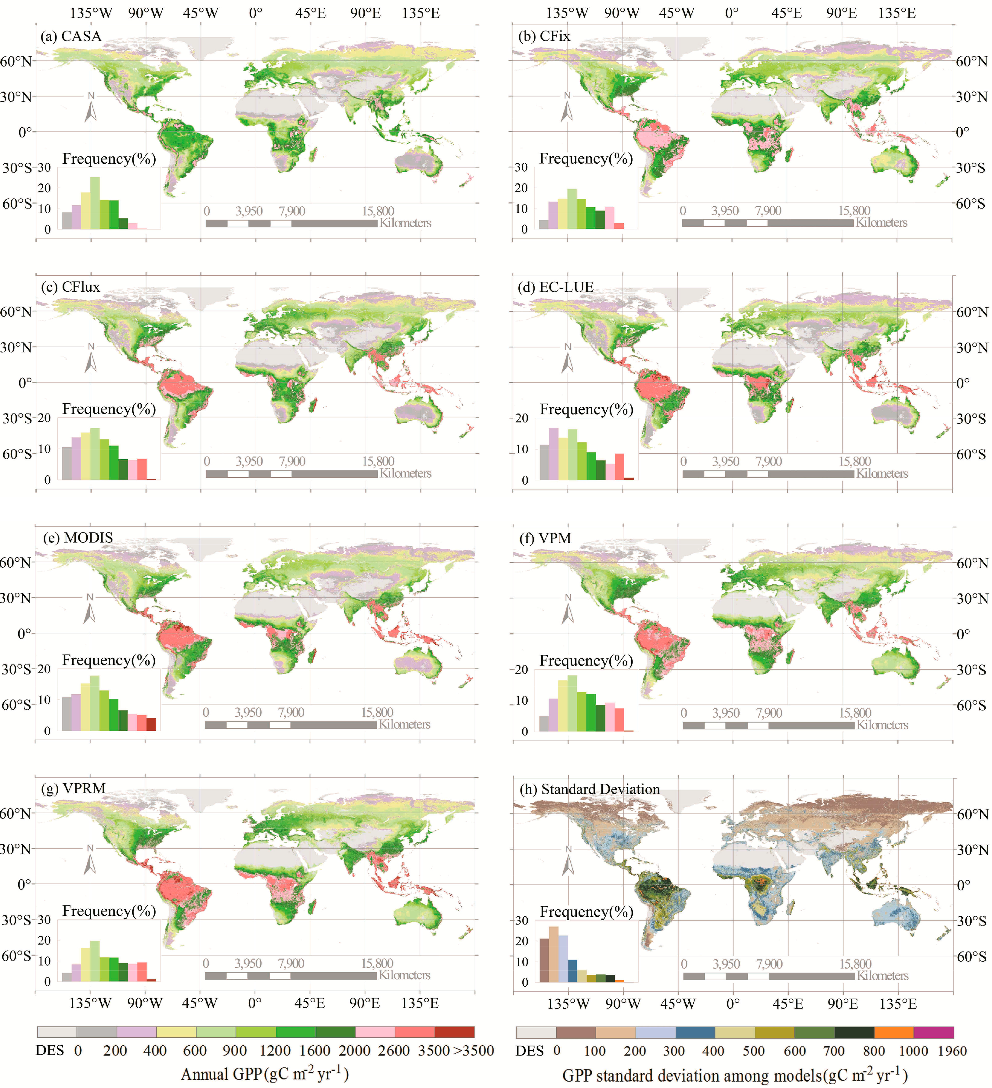
All seven LUE models showed similar spatial patterns of GPP estimates (Figure 1). The annual GPP was the highest in the humid tropics and sub-tropics, intermediate in temperate regions, and the lowest in both cold and arid regions where either temperature or water availability was the limiting factor of GPP. The seven models, however, revealed substantial differences in the GPP estimates across geographical regions and ecosystem types (Figure 1, Tables 1 and 2). For example, the CASA model simulated the lowest GPP over nearly all regions, which accounted for 68% of the highest GPP estimate from the VPRM model (Figure 1). Overall, the largest difference in the GPP estimates occurred in tropical and humid areas with high levels of production (Figure 1h). The annual GPP on the global scale ranged between 95.10 and 139.71 Pg C·yr−1, and the GPP estimates differed substantially at the various vegetation types (Tables 1 and 2). Three vegetation types (i.e., shrubland, grassland, and savanna) differed most pronounced in GPP simulations among models, as indicated by the largest coefficient of variation values (CV = 20.59%–31.07%, Table 1). Evergreen broadleaf forest, evergreen needleleaf forest, and cropland also showed considerable variability (CV = 19.07%–20.24%, Table 1). For example, evergreen broadleaf forest accounted for 22.26%–33.97% of the global GPP estimates among models, with a 19.84 Pg·C·yr−1 difference between the maximum (EC-LUE) and the minimum (CASA) GPP estimates for this type (Tables 1 and 2).
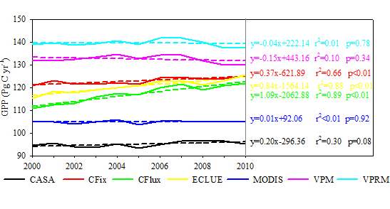
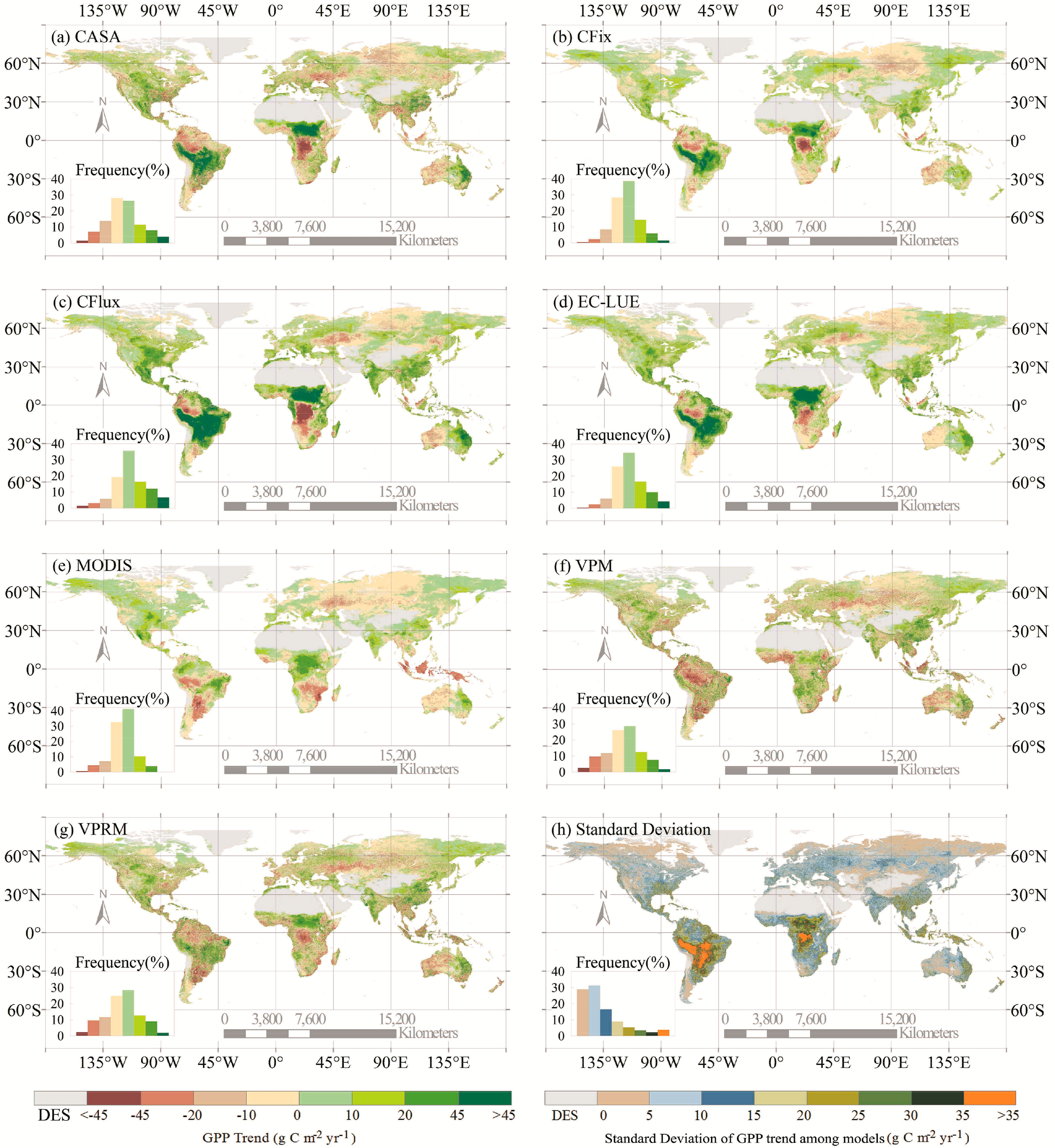
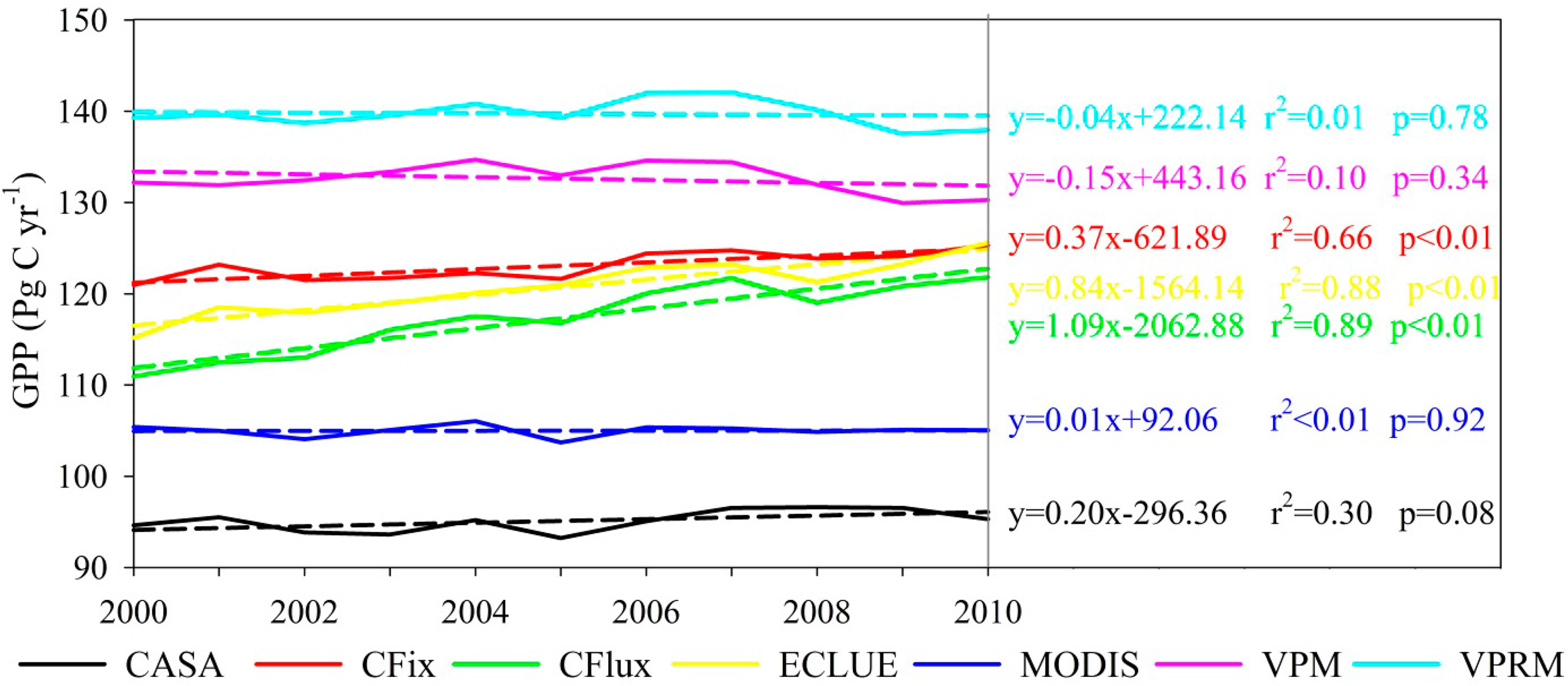
The long-term changes in GPP estimates differed among the seven LUE models (Figures 2 and 3). There were large differences in the long-term GPP trend from 2000 to 2010 over almost the entire vegetated areas of the globe (Figure 2). More than 50% of the vegetation areas had increasing GPP in more than half of the seven models (i.e., CFix, CFlux, EC-LUE, and MODIS models) (Figure 2). In terms of global annual GPP trend, three of the seven models (i.e., CFix, CFlux, and EC-LUE) showed a significant GPP increase from 2000 to 2010, with the trend ranging from 0.37 to 1.09 Pg·C·yr−1, and the largest increase of GPP was found in the CFlux model (Figure 3). The CASA and MODIS models presented relatively constant long-term change (0.20 Pg·C·yr−1, p = 0.08 and 0.01 Pg·C·yr−1, p = 0.92, respectively), and the other two models (i.e., VPM and VPRM) showed slightly decreased GPP (−0.15 Pg·C·yr−1, p = 0.34 and −0.04 Pg·C·yr−1, p = 0.78, respectively) (Figure 3).
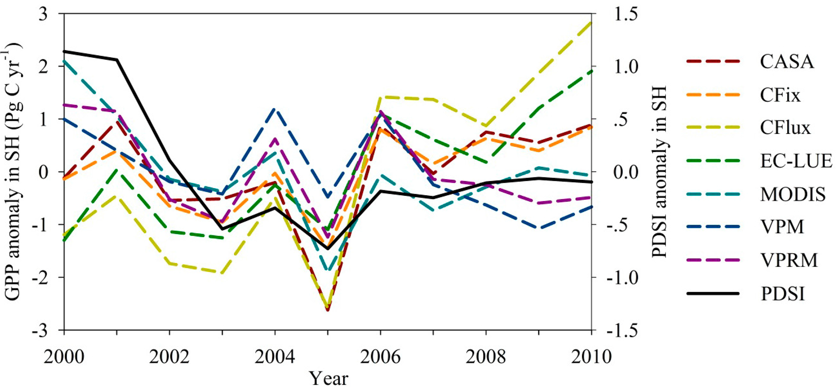
All of the seven LUE models showed the decline of GPP in 2005 and then increase trend (Figure 3). Moreover, interannual variability of GPP highly correlated with the Palmer Drought Severity Index (PDSI) in the Southern Hemisphere (Figure 4). Two models (i.e., MODIS and VPRM) showed significant correlation (r = 0.88 and 0.71, respectively, p < 0.05) between GPP and PDSI in the Southern Hemisphere. Three models (i.e., CASA, CFix, and VPM) showed weak correlation (r = 0.32–0.44, p > 0.05).
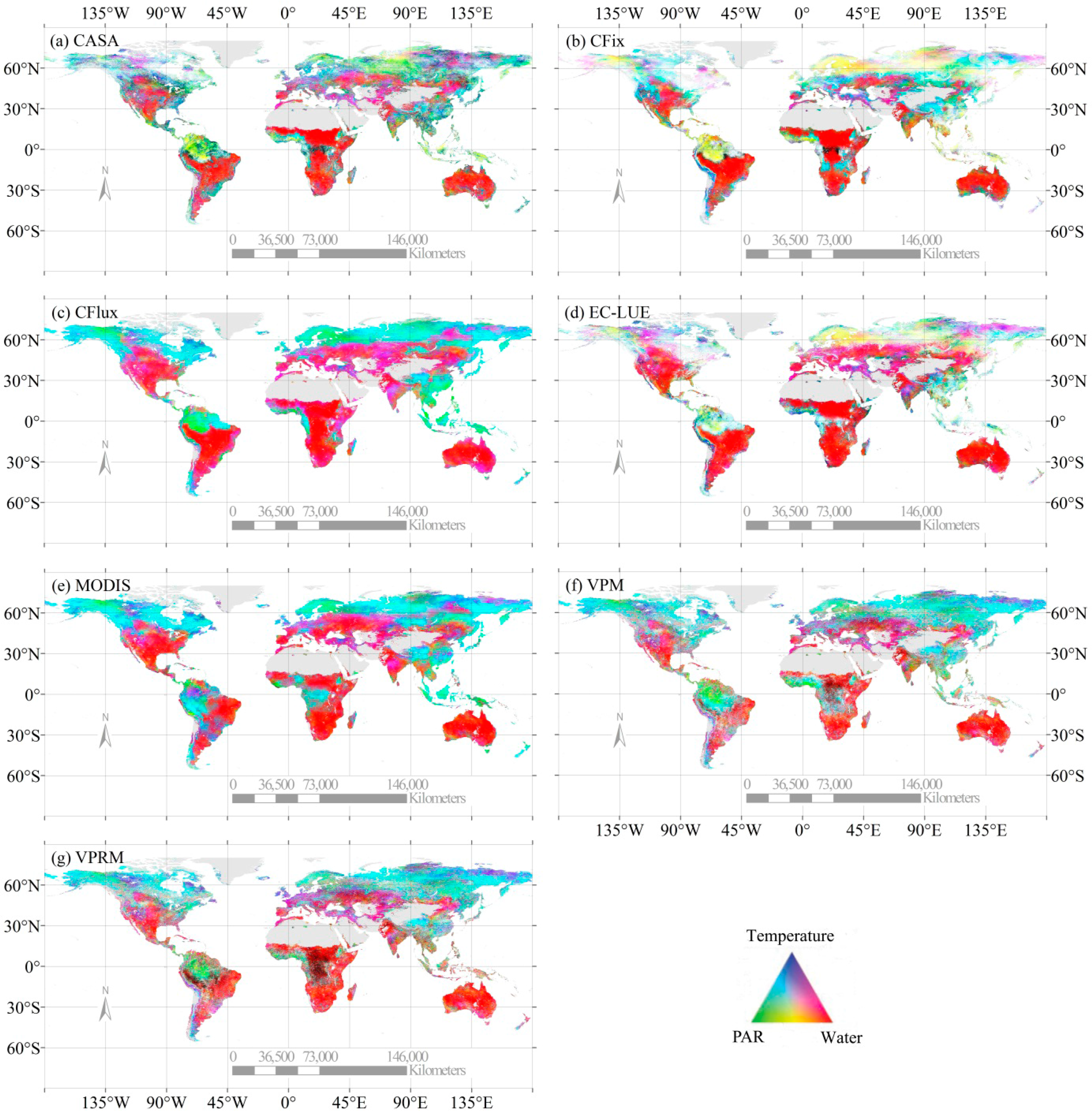
3.2. Differences in Environmental and Vegetation Regulations of the LUE Models
The simulated GPP of LUE models were regulated by many factors, including solar radiation, surface moisture, air temperature, and vegetation indices. In this study, almost all models showed strongly positive correlations between GPP and water availability (indicated by ET, inverted VPD, and LSWI) over the Southern Hemisphere, such as southern South America, Africa, Australia, and Northern arid areas, North America, and Western Europe (Figures 5 and S1–S7d). For most of the models, the air temperature dominated the GPP variability in the North high latitudes and the Tibetan Plateau (Figures 5 and S1–S7c). However, very weak temperature contributions to GPP were found over the high latitudes within the CFix and EC-LUE models (Figure 5b,d). Solar radiation played an important role in regulating the GPP interannual variability in Amazon rainforest within CASA, VPM, and VPRM models (Figure 5a,f,g). In contrast, three models (i.e., CFix, CFlux, and EC-LUE) showed strong water-dominated GPP variability over this region (Figure 5b,c,d).
Vegetation indices also played an important role in regulating the ecosystem GPP in most of the LUE models. More than half of the seven models positively correlated vegetation indices (shown by NDVI, EVI, and FPAR) with GPP estimates over more than half (i.e., 56.19%–65.02%) of the global vegetated areas (Table 3), such as Amazon, Australia, Southeast Asia, North America, and Western Europe (data not shown). In particular, CFix and EC-LUE had more vegetated areas showing positive correlations of vegetation indices with GPP compared with other models (Table 3).
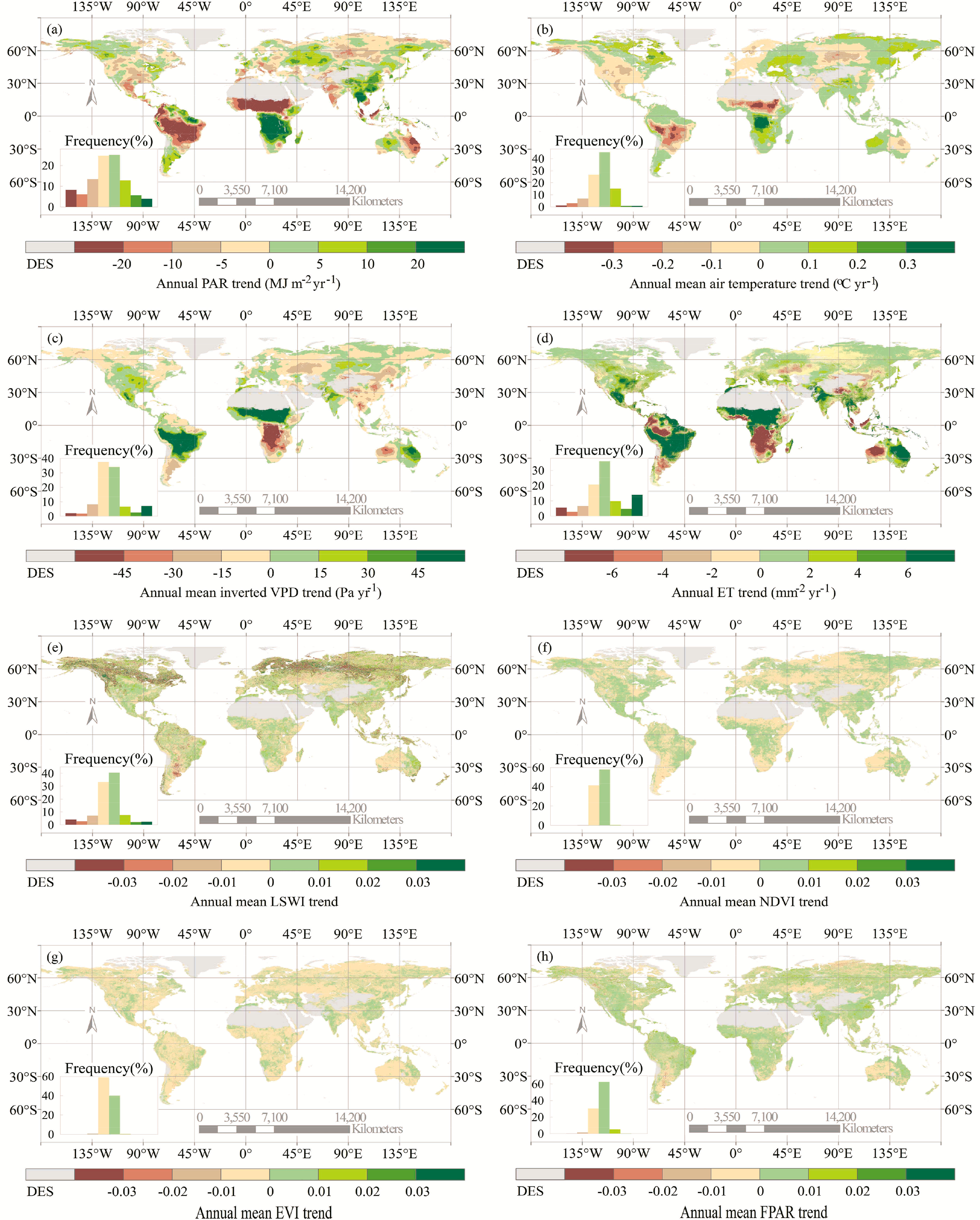
Differences in the model input variables resulted in significant differences in the interannual variability of GPP estimates among LUE models. Obvious spatial trends of the long-term GPP estimates were substantially different over the 11 years. Figure 6 showed that the key environmental variables and vegetation indices related with GPP, such as solar radiation, water availability, and air temperature, all changed significantly over the globe. Correlation analyses showed strong positive relationships between the GPP estimates and ET over large areas within the CFix, CFlux, and EC-LUE models (Figure 5b–d). This environmental variable increased between 2000 and 2010 in corresponding geographical regions (Figure 6d), which resulted in interannual variations of GPP estimates. At areas such as the southern South America, South Africa, North America, and Southeast Asia, GPP estimates were correlated with ET in the three models, and the increased ET led to consistent GPP increase (Figure 4b–d).
4. Discussion
4.1. The Differences in the Magnitude and Trend of GPP Estimates
Gross primary productivity (GPP) is the largest component flux of the global carbon cycle, and the accuracy of GPP estimates strongly determines terrestrial carbon fluxes and carbon budget [44]. A recent study shows that LUE models perform as well as the best process-based models evaluated by observations from 36 North American flux towers [45]. One of the major reasons is that LUE models are always calibrated and evaluated based on flux tower eddy covariance measurements across various geographic and climate areas [12,19–21,35,38]. The seven LUE models used in this study have utilized parameters calibrated using eddy covariance measurements [26]. The global GPP estimates of these models is 119.07 ± 15.29 Pg·C·yr−1, which is comparable to the flux-tower-based simulations of 119.4 ± 5.9 Pg·C·yr−1 and 123 ± 8 Pg·C·yr−1 using model tree ensemble approach and data-driven method, respectively [1,46]. However, large uncertainties still exist in GPP simulations by LUE models, one of which is associated with uncertainty of model input data. For instance, it is difficult to characterize water available for plants and its effect on photosynthesis over large areas from modeling, and this limits the accuracy of any spatial GPP models [26]. The estimated ET of the revised RS-PM model driven by the global MERRA meteorological data can explain 67% of the variations of annual mean ET across 54 flux sites [39], which indicates that ET model errors will further reduce the performance of LUE models [47].
Therefore, though site-scale model parameterization and evaluation can improve the performance of LUE models, large differences still exist over the global scale. These large differences are unexpected because all models have been calibrated. Difference in model formulations is probably a major cause. Previous studies have shown that different GPP estimates among models are caused by model structural differences [48–50]. For example, changes in the formulations of LUE models result in large differences in the spatial pattern of the simulated GPP [49]. Changes in the model structures will change the model outputs, as suggested by inter-comparison of 26 models, including 6 LUE models [50]. Our study showed that GPP simulations of shrubland, grassland, and savanna differed most pronounced among models (Tables 1 and 2). These ecosystems are vulnerable to water limitation. Previous study has revealed water stress algorithms generate the largest variation among models compared to temperature factors [26]. Hence, the GPP difference of these ecosystems may be attributed to the model discrepancy in quantifying water stress. GPP of evergreen broadleaf forest and cropland also showed large differences among models (Tables 1 and 2). Plant photosynthesis of evergreen broadleaf forest is jointly determined by various environmental variables, increasing the difficulty in modeling [26,51]. Cropland is heavily influenced by complex anthropogenic activities, which is not formulated into models [52,53]. Therefore, it is necessary to conduct model inter-comparison to understand the impacts of algorithms of LUE models on GPP estimates [48,54].
The interannual variability of GPP estimates also differed among the seven models from the spatial perspective. Several site-based studies have revealed the same conclusion [26,33,45]. For example, a model comparison, which assessed the performance of 16 terrestrial biosphere models and 3 remote sensing products at 11 forested sites in North America, has found that none of the models consistently reproduce the observed interannual variability [33]. Large difference in environmental regulations and vegetation indices is one of the major causes (see Sections 4.2 and 4.3).
4.2. Differences in Environmental Regulations of LUE Models
Terrestrial ecosystem GPP variations are primarily determined by changes in environmental drivers, such as solar radiation, air temperature, water availability, and vegetation indices, because GPP estimates of LUE models mainly depend on these model inputs. In this study, most of the models found strong positive correlation between GPP estimates and the water availability across large areas and various ecosystems (Figure 5). Our results are consistent with previous global and regional studies. A study has confirmed that water availability influences the vegetation photosynthesis in 40% of the global vegetated areas in recent years [1]. At the regional scale, the spatial variations of annual GPP are positively influenced by rainfall and ET, as evaluated at 35 eddy covariance flux sites [55]. Net ecosystem production has decreased with reduced water availability observed at 14 European sites [56]. However, different LUE models showed varied areas displaying a positive correlation of water availability and GPP estimates (Table 3). Therefore, it can be inferred that different LUE models will give varied GPP estimates in the future, due to varied projections of the ecosystem water balance [57].
We found a negative correlation between GPP and solar radiation, particularly in savanna, shrubland, and grassland across the globe (Figures S1–S7b and S8), which may indicate an additional indirect effect of radiation or temperature on GPP through the water balance [58]. High levels of radiation are usually associated with high temperature and high evapotranspiration rates, which exert high stomatal conductance on the vegetation canopy and thus yield high water stress for primary production in these water-limited ecosystems [1] and vice versa. Therefore, the interannual variability of the CO2 exchange in savanna, shrubland, and grassland ecosystems depends upon the duration of the wet season [59–61]. In our study, we found that radiation and water availability showed contrasting trends in these ecosystems, and the latter positively correlated with GPP (Figures S1–S7b,d), indicating that water availability plays a more important role than radiation in regulating the GPP variability due to the above interactions between water and radiation.
There are debates on the impacts of radiation and drought on vegetation production in Amazon rainforest. The seven LUE models exhibited different effects of environmental variables on GPP estimates at Amazon (Figure 5). Three models (i.e., CFix, CFlux, and EC-LUE) showed that water dominated the GPP variations in this region (Figure 5b,c,d). Other lines of results support this conclusion that drought in Amazon area decreased the GPP [62–64]. For example, Amazon Basin accumulated 1.2–1.6 Pg·C·yr−1 less carbon during the drought period of 2004–2005 than in previous years [62]. In contrast, CASA, VPM, and VPRM models exhibited an important role of solar radiation in regulating GPP estimates in Amazon rainforest. The decreased GPP estimates at this region are due to declined radiation for plants (Figures 5a,f,g, and 6a).
Despite the large difference of water regulations on GPP estimates among models, all of the seven LUE models showed the decline of global annual GPP estimates in 2005 (Figure 3). Previous studies have reported the strong impacts of large-scale drought on vegetation production over the Southern Hemisphere, and resulted into the substantial reduction of global vegetation production [3,65]. In this study, all seven models estimate the same decreased GPP in 2005, which implies the high confidence of model estimates. Our results also support the previous studies that drought is a major cause for the GPP anomaly in 2005 (Figure 4).
Temperature shows an important influence on vegetation production at high latitudes because it is a limiting factor for plants in these regions [66]. All of the LUE models in this study integrate the impact of temperature on GPP. Our results showed that air temperature dominated the GPP variations in boreal areas in most of the models (Figure 5). This is consistent with previous studies. For example, increasing temperature may stimulate GPP due to a lengthened growing season in these regions [67].
4.3. Differences in Vegetation Regulations of LUE Models
The LUE-type models are predominantly applied in satellite-based models, where the fraction of solar radiation intercepted by terrestrial vegetation (FPAR) is calculated from remote sensing data. In this study, FPAR was either a MODIS product (MOD15) or was derived from NDVI and EVI. Although NDVI and EVI are complementary vegetation indices [68], there was a remarkable difference in the long-term change between NDVI and EVI over the global scale (Figure 6f,g). The NDVI is the integration of near infrared (NIR) and red reflectance bands, while the EVI is the composition of three reflectance bands including NIR, red, and blue bands. Difference of the interannual variability of the reflectance bands may cause different NDVI and EVI trends [68–70]. We recommend that future studies may quantitative analyze the possible reasons for the differences in the long-term changes of vegetation indices.
5. Conclusions
We compared seven LUE models (CASA, CFix, CFlux, EC-LUE, MODIS, VPM, and VPRM) for simulating terrestrial ecosystem GPP over the period 2000–2010, and our results revealed large discrepancies among models. Though calibrated by the observations from FLUXNET sites, LUE models estimated terrestrial GPP with large differences in the magnitude, spatial, and temporal variation. Differences in model formulations and model drivers can cause large discrepancies in the spatial and temporal changes of GPP estimates. In particular, water availability (indicated by ET, inverted VPD, and LSWI) and vegetation conditions (shown by NDVI, EVI, and FPAR) played more important roles than radiation and air temperature in regulating interannual variability of GPP across large vegetated areas, including the Amazon, South Africa, Australia, Southeast Asia, North America, and Western Europe. Although the LUE models have significant advantages, such as the simplicity of implementation and the ability to combine remotely sensed data, they are limited in considering the various impacts on plant photosynthesis. To improve our understanding of terrestrial GPP, model inter-comparison has been performed at the global scale and a comprehensive analysis revealing differences of global GPP estimates has been conducted. Our study suggested that LUE models need to examine the representation of vegetation indices and the nonlinear functional dependencies of GPP on environmental drivers, especially water availability.
Supplementary Information
remotesensing-06-08945-s001.pdfAcknowledgments
This study was supported by the National Science Foundation for Excellent Young Scholars of China (41322005), the National High Technology Research and Development Program of China (863 Program) (2013AA122003), the National Natural Science Foundation of China (41201078), the Program for New Century Excellent Talents in University (NCET-12-0060), and the Fundamental Research Funds for the Central Universities.
Author Contributions
Wenwen Cai performed the research reported in this paper and wrote the manuscript. Wenping Yuan, Shuguang Liu, Shunlin Liang and Wenjie Dong contributed to the development and refinement of the manuscript. Yang Chen simulated the global ET data. Dan Liu and Haicheng Zhang downloaded all of the data sets used for model runs.
Conflict of Interest
The authors declare no conflict of interest.
References
- Beer, C.; Reichstein, M.; Tomelleri, E.; Ciais, P.; Jung, M.; Carvalhais, N.; Rödenbeck, C.; Arain, M.A.; Baldocchi, D.; Bonan, G.B.; et al. Terrestrial gross carbon dioxide uptake: Global distribution and covariation with climate. Science 2010, 329, 834–838. [Google Scholar]
- Raupach, M.R.; Canadell, J.G.; Le Quéré, C. Anthropogenic and biophysical contributions to increasing atmospheric CO2 growth rate and airborne fraction. Biogeosciences 2008, 5, 1601–1613. [Google Scholar]
- Zhao, M.; Running, S.W. Drought-induced reduction in global terrestrial net primary production from 2000 through 2009. Science 2010, 329, 940–943. [Google Scholar]
- Prince, S.D.; Goward, S.N. Global primary production: A remote sensing approach. J. Biogeogr 1995, 22, 815–835. [Google Scholar]
- Ruimy, A.; Dedieu, G.; Saugier, B. TURC: A diagnostic model of continental gross primary productivity and net primary productivity. Glob. Biogeochem. Cycles 1996, 10, 269–285. [Google Scholar]
- Landsberg, J.J.; Waring, R.H.; Coops, N.C. Performance of the forest productivity model 3-PG applied to a wide range of forest types. For. Ecol. Manag 2003, 172, 199–214. [Google Scholar]
- Cramer, W.; Kicklighter, D.W.; Bondeau, A.; Moore, B., III; Churkina, G.; Nemry, B.; Ruimy, A.; Schioss, A.L. The participants of the Potsdam NPP Model Intercomparison. Comparing global models of terrestrial net primary productivity (NPP): Overview and key results. Glob. Chang. Biol 1999, 5, 1–15. [Google Scholar]
- Jung, M.; Vetter, M.; Herold, M.; Churkina, G.; Reichstein, M.; Zaehle, S.; Ciais, P.; Viovy, N.; Bondeau, A.; Chen, Y.; et al. Uncertainties of modeling gross primary productivity over Europe: A systematic study on the effects of using different drivers and terrestrial biosphere models. Glob. Biogeochem. Cycles 2007, 21, 1–12. [Google Scholar]
- Ichii, K.; Kondo, M.; Lee, Y.-H.; Wang, S.-Q.; Kim, J.; Ueyama, M.; Lim, H.-J.; Shi, H.; Suzuki, T.; Ito, A.; et al. Site-level model-data synthesis of terrestrial carbon fluxes in the CarboEastAsia eddy-covariance observation network: Toward future modeling efforts. J. For. Res 2012, 18, 13–20. [Google Scholar]
- Monteith, J.L. Solar radiation and productivity in tropical ecosystems. J. Appl. Ecol 1972, 9, 747–766. [Google Scholar]
- Field, C.B.; Randerson, J.T.; Malmström, C.M. Global net primary production: Combining ecology and remote sensing. Remote Sens. Environ 1995, 51, 74–88. [Google Scholar]
- Running, S.W; Neman, R.R.; Heinsch, F.A.; Zhao, M.; Reeves, M.; Hashimoto, H. A continuous satellite-derived measure of global terrestrial primary production. BioScience 2004, 54, 547–560. [Google Scholar]
- Yuan, W.; Liu, D.; Dong, W.; Liu, S.; Zhou, G.; Yu, G.; Zhao, T.; Feng, J.; Ma, Z.; Chen, J.; et al. Multiyear precipitation reduction strongly decreases carbon uptake over northern China. J. Geophys. Res 2014, 119, 881–896. [Google Scholar]
- Cai, W.; Yuan, W.; Liang, S.; Zhang, X.; Dong, W.; Xia, J.; Fu, Y.; Chen, Y.; Liu, D.; Zhang, Q. Improved estimations of gross primary production using satellite-derived photosynthetically active radiation. J. Geophys. Res 2014, 119, 110–123. [Google Scholar]
- Landsberg, J.J.; Waring, R.H. A generalised model of forest productivity using simplified concepts of radiation-use efficiency, carbon balance and partitioning. For. Ecol. Manag 1997, 95, 209–228. [Google Scholar]
- Law, B.E.; Williams, M.; Anthoni, P.M.; Baldocchi, D.D.; Unsworth, M.H. Measuring and modeling seasonal variation of carbon dioxide and water vapor exchange of a pinus ponderosa forest subject to soil water deficit. Glob. Chang. Biol 2000, 6, 613–630. [Google Scholar]
- Coops, N.C.; Ferster, C.J.; Waring, R.H.; Nightingale, J. Comparison of three models for predicting gross primary production across and within forested ecoregions in the contiguous United States. Remote Sens. Environ 2009, 113, 680–690. [Google Scholar]
- Potter, C.S.; Randerson, J.T.; Field, C.B.; Matson, P.A.; Vitousek, P.M.; Mooney, H.A.; Klooster, S.A. Terrestrial ecosystem production: A process model based on global satellite and surface data. Glob. Biogeochem. Cycles 1993, 7, 811–841. [Google Scholar]
- Xiao, X.; Hollinger, D.; Aber, J.; Goltz, M.; Davidson, E.A.; Zhang, Q.; Moore, B., III. Satellite-based modeling of gross primary production in an evergreen needleleaf forest. Remote Sens. Environ 2004, 89, 519–534. [Google Scholar]
- Turner, D.P.; Ritts, W.D.; Styles, J.M.; Yang, Z.; Cohen, W.B.; Law, B.E.; Thornton, P.E. A diagnostic carbon flux model to monitor the effects of disturbance and interannual variation in climate on regional NEP. Tellus 2006, 58B, 476–490. [Google Scholar]
- Mahadevan, P.; Wofsy, S.C.; Matross, D.M.; Xiao, X.; Dunn, A.L.; Lin, J.C.; Gerbig, C.; Munger, J.W.; Chow, V.Y.; Gottlieb, E.W. A satellite-based biosphere parameterization for net ecosystem CO2 exchange: Vegetation photosynthesis and respiration model (VPRM). Glob. Biogeochem. Cycles 2008, 22. [Google Scholar] [CrossRef]
- Chen, Y.; Xia, J.; Liang, S.; Feng, J.; Fisher, J.; Li, X.; Li, X.; Liu, S.; Ma, Z.; Miyata, A.; et al. Comparison of satellite-based evapotranspiration models over terrestrial ecosystems in China. Remote Sens. Environ 2014, 140, 279–293. [Google Scholar]
- Heinsch, F.A.; Zhao, M.; Running, S.W.; Kimball, J.S.; Nemani, R.R.; Davis, K.J.; Bolstad, P.V.; Cook, B.D.; Desai, A.R.; Ricciuto, D.M.; et al. Evaluation of remote sensing based terrestrial productivity from MODIS using regional tower eddy flux network observations. IEEE Trans. Geosci. Remote Sens 2006, 44, 1908–1925. [Google Scholar]
- Desai, A.R.; Richardson, A.D.; Moffat, A.M.; Kattge, J.; Hollinger, D.Y.; Barr, A.; Falge, E.; Noormets, A.; Papale, D.; Reichstein, M.; et al. Cross-site evaluation of eddy covariance GPP and RE decomposition techniques. Agric. For. Meteorol 2008, 148, 821–838. [Google Scholar]
- Li, X.; Liang, S.; Yu, G.; Yuan, W.; Cheng, X.; Xia, J.; Zhao, T.; Feng, J.; Ma, Z.; Ma, M.; et al. Estimation of gross primary production over the terrestrial ecosystems in China. Ecol. Model 2013, 261–262, 80–92. [Google Scholar]
- Yuan, W.; Cai, W.; Xia, J.; Chen, J.; Liu, S.; Dong, W.; Merbold, L.; Law, B.; Arain, A.; Beringer, J.; et al. Global comparison of light use efficiency models for simulating terrestrial vegetation gross primary production based on the LaThuile database. Agric. For. Meteorol 2014, 192–193, 108–120. [Google Scholar]
- Chapin, F.S., III; Matson, P.A.; Vitousek, P. Carbon inputs to ecosystems. In Principles of Terrestrial Ecosystem Ecology, 2nd ed.; Springer: New York, NY, USA, 2011; pp. 123–156. [Google Scholar]
- Yuan, W.; Liu, S.; Dong, W.; Liang, S.; Zhao, S.; Chen, J.; Xu, W.; Li, X.; Barr, A.; Black, T.; et al. Differentiating moss from higher plants is critical in studying the carbon cycle of the boreal biome. Nat. Commun 2014, 5. [Google Scholar] [CrossRef]
- Yuan, W.; Liu, S.; Liang, S.; Tan, Z.; Liu, H.; Young, C. Estimations of evapotranspiration and water balance with uncertainty over the Yukon River Basin. Water Resour. Manag 2012, 26, 2147–2157. [Google Scholar]
- Nightingale, J.M.; Coops, N.C.; Waring, R.H.; Hargrove, W.W. Comparison of MODIS gross primary production estimates for forests across the U.S.A. with those generated by a simple process model, 3-PGS. Remote Sens. Environ 2007, 109, 500–509. [Google Scholar]
- Joseph, S.; van Laake, P.E.; Thomas, A.P.; Eklundh, L. Comparison of carbon assimilation estimates over tropical forest types in India based on different satellite and climate data products. Int. J. Appl. Earth Obs. Geoinf 2012, 18, 557–563. [Google Scholar]
- Huntzinger, D.N.; Post, W.M.; Wei, Y.; Michalak, A.M.; West, T.O.; Jacobson, A.R.; Baker, I.T.; Chen, J.M.; Davis, K.J.; Hayes, D.J.; et al. North American Carbon Program (NACP) regional interim synthesis: Terrestrial biospheric model intercomparison. Ecol. Model 2012, 232, 144–157. [Google Scholar]
- Keenan, T.; Baker, I.; Barr, A.; Ciais, P.; Davis, K.; Dietze, M.; Dragoni, D.; Gough, C.M.; Grant, R.; Hollinger, D. Terrestrial biosphere model performance for inter-annual variability of land-atmosphere CO2 exchange. Glob. Chang. Biol 2012, 18, 1971–1987. [Google Scholar]
- Van der Werf, G.R.; Randerson, J.T.; Collatz, G.J.; Giglio, L. Carbon emissions from fires in tropical and subtropical ecosystems. Glob. Chang. Biol 2003, 9, 547–562. [Google Scholar]
- Veroustraete, F.; Sabbe, H.; Eerens, H. Estimation of carbon mass fluxes over Europe using the C-Fix model and Euroflux data. Remote Sens. Environ 2002, 83, 376–399. [Google Scholar]
- Verstraeten, W.W.; Veroustraete, F.; Feyen, J. On temperature and water limitation of net ecosystem productivity: Implementation in the C-Fix model. Ecol. Model 2006, 199, 4–22. [Google Scholar]
- King, D.A.; Turner, D.P.; Ritts, W.D. Parameterization of a diagnostic carbon cycle model for continental scale application. Remote Sens. Environ 2011, 115, 1653–1664. [Google Scholar]
- Yuan, W.; Liu, S.; Zhou, G.; Zhou, G.Y.; Tieszen, L.L.; Baldocchi, D.; Bernhofer, C.; Gholz, H.; Goldstein, A.H.; Goulden, M.L.; et al. Deriving a light use efficiency model from eddy covariance flux data for predicting daily gross primary production across biomes. Agric. For. Meteorol 2007, 143, 198–207. [Google Scholar]
- Yuan, W.; Liu, S.; Yu, G.; Bonnefond, J.-M.; Chen, J.; Davis, K.; Desai, A.R.; Goldstein, A.H.; Gianelle, D.; Rossi, F.; et al. Global estimates of evapotranspiration and gross primary production based on MODIS and global meteorology data. Remote Sens. Environ 2010, 114, 1416–1431. [Google Scholar]
- Global Modeling and Assimilation Office (GMAO); Goddard Space Flight Center. File Specification for GEOS-5 DAS Gridded Output. Available online: http://gmao.gsfc.nasa.gov/ (accessed on 18 January 2012).
- Zhao, M.; Heinsch, F.A.; Nemani, R.R.; Running, S.W. Improvements of the MODIS terrestrial gross and net primary production global data set. Remote Sens. Environ 2005, 95, 164–176. [Google Scholar]
- Holben, B.N. Characteristics of maximum-value composite images from temporal AVHRR data. Int. J. Remote Sens 1986, 7, 1417–1434. [Google Scholar]
- United States Geological Survey (USGS). General Cartographic Transformation Package (GCTP). Available online: http://gcmd.nasa.gov/records/USGS-GCTP.html (accessed on 12 October 2011).
- Canadell, J.G.; Mooney, H.A.; Baldocchi, D.D.; Berry, J.A.; Ehleringer, J.R.; Field, C.B.; Gower, S.T.; Hollinger, D.Y.; Hunt, J.E.; Jackson, R.B.; et al. Carbon metabolism of the terrestrial biosphere: A multitechnique approach for improved understanding. Ecosystems 2000, 3, 115–130. [Google Scholar]
- Raczka, B.M.; Davis, K.J.; Huntzinger, D.; Neilson, R.P.; Poulter, B.; Richardson, A.D.; Xiao, J.; Baker, I.; Ciais, P.; Keenan, T.F.; et al. Evaluation of continental carbon cycle simulations with North American flux tower observations. Ecol. Monogr 2013, 83, 531–556. [Google Scholar]
- Jung, M.; Reichstein, M.; Margolis, H.A.; Cescatti, A.; Richardson, A.D.; Arain, M.A.; Arneth, A.; Bernhofer, C.; Bonal, D.; Chen, J.; et al. Global patterns of land-atmosphere fluxes of carbon dioxide, latent heat, and sensible heat derived from eddy covariance, satellite, and meteorological observations. J. Geophys. Res 2011, 116, G00J07. [Google Scholar]
- Mu, Q.; Zhao, M.; Kimball, J.S.; McDowell, N.G.; Running, S.W. A remotely sensed global terrestrial drought severity index. Bull. Am. Meteorol. Soc 2013, 94, 83–98. [Google Scholar]
- Ogutu, B.O.; Dash, J. Assessing the capacity of three production efficiency models in simulating gross carbon uptake across multiple biomes in conterminous USA. Agric. For. Meteorol 2013, 174–175, 158–169. [Google Scholar]
- McCallum, I.; Franklin, O.; Moltchanova, E.; Merbold, L.; Schmullius, C.; Shvidenko, A.; Schepaschenko, D.; Fritz, S. Improved light and temperature responses for light-use-efficiency-based GPP models. Biogeosciences 2013, 10, 6577–6590. [Google Scholar]
- Schaefer, K.; Schwalm, C.R.; Williams, C.; Arain, M.A.; Barr, A.; Chen, J.M.; Davis, K.J.; Dimitrov, D.; Hilton, T.W.; Hollinger, D.Y.; et al. A model-data comparison of gross primary productivity: Results from the North American Carbon Program site synthesis. J. Geophys. Res 2012, 117, G03010. [Google Scholar]
- Xiao, X.; Zhang, Q.; Saleska, S.; Hutyra, L.; Camargo, P.D.; Wofsy, S.; Frolking, S.; Boles, S.; Keller, M.; Moore, B., III. Satellite-based modeling of gross primary production in a seasonally moist tropical evergreen forest. Remote Sens. Environ 2005, 94, 105–112. [Google Scholar]
- Guanter, L.; Zhang, Y.; Jung, M.; Joiner, J.; Voigt, M.; Berry, J.A.; Frankenberg, C.; Huete, A.R.; Zarco-Tejada, P.; Lee, J.-E.; et al. Global and time-resolved monitoring of crop photosynthesis with chlorophyll fluorescence. Proc. Natl. Acad. Sci. USA 2014, 111, E1327–E1333. [Google Scholar]
- Bradford, J.B.; Hicke, J.A.; Lauenroth, W.K. The relative importance of light-use efficiency modifications from environmental conditions and cultivation for estimation of large-scale net primary productivity. Remote Sens. Environ 2005, 96, 246–255. [Google Scholar]
- Vinukollu, R.K.; Meynadier, R.; Sheffield, J.; Wood, E.F. Multi-model, multi-sensor estimates of global evapotranspiration: Climatology, uncertainties and trends. Hydrol. Process 2011, 25, 3993–4410. [Google Scholar]
- Garbulsky, M.F.; Peñuelas, J.; Papale, D.; Ardö, J.; Goulden, M.L.; Kiely, G.; Richardson, A.D.; Rotenberg, E.; Veenendaal, E.M.; Filella, I. Patterns and controls of the variability of radiation use efficiency and primary productivity across terrestrial ecosystems. Glob. Ecol. Biogeogr 2010, 19, 253–267. [Google Scholar]
- Granier, A.; Reichstein, M.; Bréda, N.; Janssens, I.A.; Falge, E.; Ciais, P.; Grünwald, T.; Aubinet, M.; Berbigier, P.; Bernhofer, C.; et al. Evidence for soil water control on carbon and water dynamics in European forests during the extremely dry year: 2003. Agric. For. Meteorol 2007, 143, 123–145. [Google Scholar]
- IPCC. Summary for policymakers. In Climate Change 2013: The Physical Science Basis Contribution of Working Group I to the Fifth Assessment Report of the Intergovernmental Panel on Climate Change; Stocker, T.F., Qin, D., Plattner, G.K., Tignor, M., Allen, S.K., Boschung, J., Nauels, A., Xia, Y., Bex, V., Midgley, P.M., Eds.; Cambridge University Press: Cambridge, UK/Cambridge, NY, USA, 2012; pp. 3–29. [Google Scholar]
- Beer, C.; Reichstein, M.; Ciais, P.; Farquhar, G.D.; Papale, D. Mean annual GPP of Europe derived from its water balance. Geophys. Res. Lett 2007, 34, L05401. [Google Scholar]
- Luo, H.; Oechel, W.C.; Hastings, S.J.; Zulueta, R.; Qian, Y.; Kwon, H. Mature semiarid chaparral ecosystems can be a significant sink for atmospheric carbon dioxide. Glob. Chang. Biol 2007, 13, 386–396. [Google Scholar]
- Ma, S.; Baldocchi, D.D.; Xu, L.; Hehn, T. Inter-annual variability in carbon dioxide exchange of an oak/grass savanna and open grassland in California. Agric. For. Meteorol 2007, 147, 157–171. [Google Scholar]
- Paw, U.K.T.; Falk, M.; Suchanek, T.H.; Ustin, S.L.; Chen, J.; Park, Y.-S.; Winner, W.E.; Thomas, S.C.; Hsiao, T.C.; Shaw, R.H.; et al. Carbon dioxide exchange between an old-growth forest and the atmosphere. Ecosystems 2004, 7, 513–524. [Google Scholar]
- Phillips, O.L.; Aragão, L.E.O.C.; Lewis, S.L.; Fisher, J.B.; Lloyd, J.; López-González, G.; Malhi, Y.; Monteagudo, A.; Peacock, J.; Quesada, C.A.; et al. Drought sensitivity of the Amazon rainforest. Science 2009, 323, 1344–1347. [Google Scholar]
- Lewis, S.L.; Brando, P.M.; Phillips, O.L.; van der Heijden, G.M.F.; Nepstad, D. The 2010 Amazon drought. Science 2011, 331. [Google Scholar] [CrossRef]
- Lee, J.-E.; Frankenberg, C.; van der Tol, C.; Berry, J.A.; Guanter, L.; Boyce, C.K.; Fisher, J.B.; Morrow, E.; Worden, J.R.; Asefi, S.; et al. Forest productivity and water stress in Amazonia: Observations from GOSAT chlorophyll fluorescence. Proc. R. Soc. B 2013, 280. [Google Scholar] [CrossRef]
- Meir, P.; Brando, P.M.; Nepstad, D.; Vasconcelos, S.; Costa, A.C.L.; Davidson, E.; Almeida, S.; Fisher, R.A.; Sotta, E.D.; Zarin, D.; et al. The effects of drought on Amazonian rain forests. In Amazonia and Global Change; Keller, M., Bustamante, M., Gash, J., Dias, P.S., Eds.; American Geophysical Union: Washington, DC, USA, 2013; pp. 429–449. [Google Scholar]
- Baldocchi, D. Breathing of the terrestrial biosphere: Lessons learned from a global network of carbon dioxide flux measurement systems. Aust. J. Bot 2008, 56, 1–26. [Google Scholar]
- Flanagan, L.B.; Syed, K.H. Stimulation of both photosynthesis and respiration in response to warmer and drier conditions in a boreal peatland ecosystem. Glob. Chang. Biol 2011, 17, 2271–2287. [Google Scholar]
- Huete, A.; Didan, K.; Miura, T.; Rodriguez, E.P.; Gao, X.; Ferreira, L.G. Overview of the radiometric and biophysical performance of the MODIS vegetation indices. Remote Sens. Environ 2002, 83, 195–213. [Google Scholar]
- Zhou, L.; Tian, Y.; Myneni, R.B.; Ciais, P.; Saatchi, S.; Liu, Y.Y.; Piao, S.; Chen, H.; Vermote, E.F.; Song, C.; et al. Widespread decline of Congo rainforest greenness in the past decade. Nature 2014, 509, 86–90. [Google Scholar]
- Forkel, M.; Carvalhais, N.; Verbesselt, J.; Mahecha, M.; Neigh, C.; Reichstein, M. Trend change detection in NDVI time series: Effects of inter-annual variability and methodology. Remote Sens 2013, 5, 2113–2144. [Google Scholar]


| GPP | CASA | CFix | CFlux | EC-LUE | MODIS | VPM | VPRM | CV (%) |
|---|---|---|---|---|---|---|---|---|
| ENF | 4.63 | 3.92 | 4.67 | 4.23 | 4.01 | 2.72 | 2.88 | 20.24 |
| EBF | 21.17 | 32.52 | 36.19 | 41.00 | 35.31 | 36.94 | 40.31 | 19.17 |
| DNF | 1.86 | 1.87 | 1.99 | 2.00 | 1.75 | 1.59 | 1.71 | 8.23 |
| DBF | 3.11 | 4.23 | 4.24 | 4.43 | 3.49 | 4.30 | 4.39 | 12.76 |
| MIF | 6.82 | 7.10 | 8.66 | 8.11 | 6.63 | 6.86 | 7.36 | 10.22 |
| SHR | 9.75 | 10.31 | 8.15 | 7.24 | 6.77 | 11.14 | 11.61 | 20.59 |
| SAV | 25.68 | 33.97 | 29.50 | 18.15 | 15.23 | 35.85 | 20.58 | 31.07 |
| GRA | 8.14 | 10.71 | 7.44 | 6.88 | 6.52 | 12.00 | 11.96 | 26.35 |
| CRO | 13.95 | 18.43 | 16.44 | 15.55 | 14.27 | 21.20 | 22.40 | 19.07 |
| Total | 95.10 | 123.07 | 117.29 | 120.71 | 104.99 | 132.61 | 139.71 | 12.85 |
ENF: evergreen needleleaf forest, EBF: evergreen broadleaf forest, DNF: deciduous needleleaf forest, DBF: deciduous broadleaf forest, MIF: mixed forest, SHR: shrubland, SAV: savanna, GRA: grassland, CRO: cropland. CV: the coefficient of variation. The unit of GPP is Pg·C·yr−1.
| Percentage (%) | CASA | CFix | CFlux | EC-LUE | MODIS | VPM | VPRM |
|---|---|---|---|---|---|---|---|
| ENF | 4.87 | 3.18 | 3.98 | 3.50 | 3.82 | 2.05 | 2.06 |
| EBF | 22.26 | 26.42 | 30.86 | 33.97 | 33.64 | 27.85 | 28.85 |
| DNF | 1.96 | 1.52 | 1.69 | 1.65 | 1.67 | 1.20 | 1.22 |
| DBF | 7.00 | 3.44 | 3.61 | 3.67 | 3.32 | 4.00 | 3.15 |
| MIF | 7.17 | 5.77 | 7.39 | 6.72 | 6.32 | 5.17 | 5.27 |
| SHR | 10.25 | 8.38 | 6.96 | 6.00 | 6.46 | 8.40 | 8.31 |
| SAV | 27.00 | 27.61 | 25.15 | 25.90 | 24.98 | 27.04 | 26.54 |
| GRA | 8.56 | 8.71 | 6.35 | 5.70 | 6.21 | 9.05 | 8.56 |
| CRO | 14.67 | 14.97 | 14.02 | 12.88 | 13.59 | 15.99 | 16.03 |
ENF: evergreen needleleaf forest, EBF: evergreen broadleaf forest, DNF: deciduous needleleaf forest, DBF: deciduous broadleaf forest, MIF: mixed forest, SHR: shrubland, SAV: savanna, GRA: grassland, CRO: cropland. The unit of GPP is Pg·C·yr−1.
| Percentage (%) | PAR a | Ta b | Water c | Vegetation d | ||||
|---|---|---|---|---|---|---|---|---|
| N e | P f | N | P | N | P | N | P | |
| CASA | 13.02 | 6.94 | 15.07 | 3.66 | 0.45 | 25.70 | 0.75 | 35.42 |
| CFix | 12.66 | 36.26 | 17.37 | 16.06 | 0.65 | 54.85 | 0.05 | 61.78 |
| CFlux | 27.40 | 22.45 | 13.39 | 9.51 | 0.20 | 80.88 | 0.30 | 49.63 |
| EC-LUE | 23.56 | 20.79 | 18.96 | 13.24 | 0.02 | 84.53 | 0.06 | 65.02 |
| MODIS | 18.11 | 12.08 | 13.78 | 13.38 | 11.27 | 23.62 | 0.55 | 30.84 |
| VPM | 6.23 | 19.21 | 7.11 | 11.14 | 0.93 | 35.43 | 0.23 | 56.19 |
| VPRM | 12.77 | 7.99 | 11.68 | 10.56 | 0.85 | 37.95 | 0.23 | 57.63 |
a:Annual photosynthetically active radiation;b:annual mean air temperature;c:water availability, indicated by annual evapotranspiration (ET) in the CASA, CFix, CFlux, and EC-LUE models, annual mean inverted Vapor Pressure Deficit (VPD) in the MODIS model, and annual mean Land Surface Water Index (LSWI) in the VPM and VPRM models;d:vegetation conditions, shown by the annual mean Normalized Difference Vegetation Index (NDVI) in the CASA, CFix, and EC-LUE models, annual mean Fraction of absorbed PAR by vegetation canopy (FPAR) in the CFlux and MODIS models, and annual mean Enhance Vegetation Index (EVI) in the VPM and VPRM models;e:significant negative correlation between annual GPP estimates and environmental variables or vegetation indices (p < 0.05);f:significant positive correlation between annual GPP estimates and environmental variables or vegetation indices (p < 0.05).
© 2014 by the authors; licensee MDPI, Basel, Switzerland This article is an open access article distributed under the terms and conditions of the Creative Commons Attribution license (http://creativecommons.org/licenses/by/3.0/).
Share and Cite
Cai, W.; Yuan, W.; Liang, S.; Liu, S.; Dong, W.; Chen, Y.; Liu, D.; Zhang, H. Large Differences in Terrestrial Vegetation Production Derived from Satellite-Based Light Use Efficiency Models. Remote Sens. 2014, 6, 8945-8965. https://doi.org/10.3390/rs6098945
Cai W, Yuan W, Liang S, Liu S, Dong W, Chen Y, Liu D, Zhang H. Large Differences in Terrestrial Vegetation Production Derived from Satellite-Based Light Use Efficiency Models. Remote Sensing. 2014; 6(9):8945-8965. https://doi.org/10.3390/rs6098945
Chicago/Turabian StyleCai, Wenwen, Wenping Yuan, Shunlin Liang, Shuguang Liu, Wenjie Dong, Yang Chen, Dan Liu, and Haicheng Zhang. 2014. "Large Differences in Terrestrial Vegetation Production Derived from Satellite-Based Light Use Efficiency Models" Remote Sensing 6, no. 9: 8945-8965. https://doi.org/10.3390/rs6098945