A Hierarchical Approach to Persistent Scatterer Network Construction and Deformation Time Series Estimation

Abstract

This paper presents a hierarchical approach to network construction and time series estimation in persistent scatterer interferometry (PSI) for deformation analysis using the time series of high-resolution satellite SAR images. To balance between computational efficiency and solution accuracy, a dividing and conquering algorithm (i.e., two levels of PS networking and solution) is proposed for extracting deformation rates of a study area. The algorithm has been tested using 40 high-resolution TerraSAR-X images collected between 2009 and 2010 over Tianjin in China for subsidence analysis, and validated by using the ground-based leveling measurements. The experimental results indicate that the hierarchical approach can remarkably reduce computing time and memory requirements, and the subsidence measurements derived from the hierarchical solution are in good agreement with the leveling data.

1. Introduction

As a newly arisen space geodetic technique, synthetic aperture radar interferometry (InSAR) is well known as an effective and powerful tool for monitoring land deformation. By analyzing the temporal deformation behavior using time series of phase signals, multi-temporal InSAR is able to mitigate the negative effects of two major limitations in conventional InSAR for deformation tracking, i.e., spatiotemporal decorrelation and atmospheric artifacts [1,2,3,4]. In the past decade, several advanced approaches to multi-temporal InSAR have been proposed to adapt to the specific applications, including permanent scatterer interferometry [1,2], small baseline subset method [3], coherent pixel technique [4], persistent scatterer interferometry (PSI) [5,6], persistent scatterer (PS) networking analysis [7,8,9,10], and temporarily coherent point InSAR [11].

Previous investigations indicate that the PS networking approach has advantages in eliminating geometric inconsistency and raising quality of deformation measurements, e.g. [7,8,9,10,11]. The network, formed by using all the PSs in a study area, contains a number of connections (i.e., arcs) between adjacent PSs. Therefore, the differential modeling of phase data can be implemented for every arc to cancel out or decrease the impact of spatially-correlated atmospheric delay and other systematic errors [7,8,9,10], thus benefiting deformation extraction by a least squares (LS) estimator. 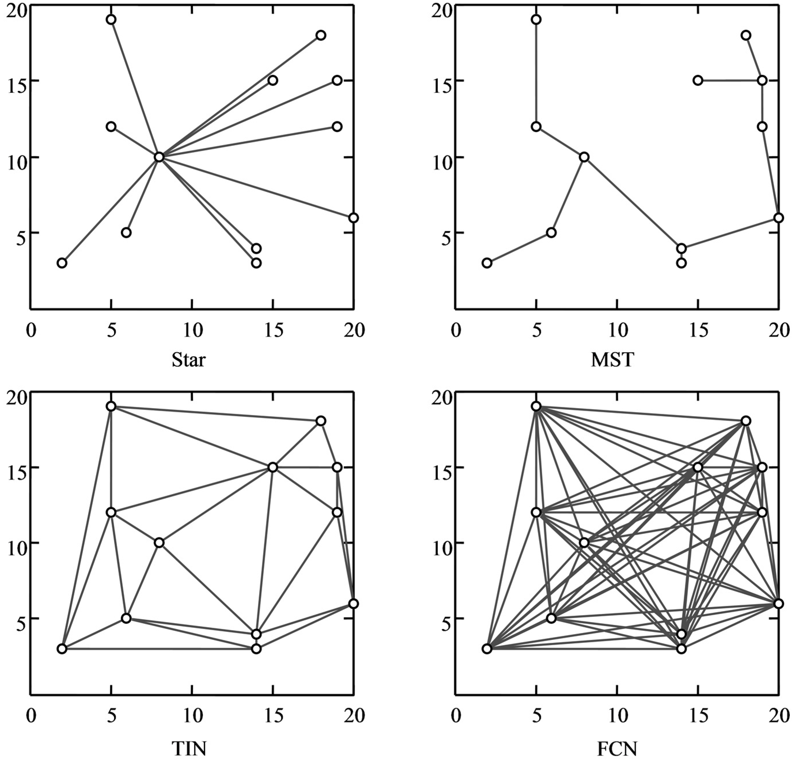As shown in Figure 1, several types of PS networks, including star network, minimum spanning tree (MST) network, triangular irregular network (TIN), and freely connected network (FCN), have been used for differential modeling and time-series deformation analysis. For the above four types of network, the former two types (i.e., star and MST) are relatively simple and cannot be used for the LS-based estimation, while the latter two types (i.e., TIN and FCN) with the redundant connections and differential phases can be used for the LS-based estimation [4,7,8,9,10,11,12,13,14]. It is understood that more connections between adjacent PSs in a network can result in a more reliable solution of deformation measurements by the LS adjustment, but decreases computational efficiency. High density of PSs for deformation analysis benefits from high-resolution SAR imagery (e.g., TerraSAR-X and COSMO-SkyMed data) [9], but the computer time and memory requirements increase significantly for the LS-based PS solution.

To balance between computational efficiency and solution accuracy, this paper presents a hierarchical approach to PS networking and solution for deformation analysis using a time series of high-resolution satellite SAR images. We propose a dividing and conquering algorithm for estimating deformation rates at all the PSs in the area of interest, in which two levels of PS network construction and LS-based solution are performed, and the results derived from the first-level analysis are used as the reference data for the second-level analysis. All the PSs in the imaged area are first divided into multiple subsets by gridding division. For the first-level solution, a global control network (GCN) is constructed by using the feature PSs in each grid cell (see Section 2.2.1). The feature PSs mean having high signal-to-noise ratio (SNR) in phase measurements and they are empirically selected as the primary control points (PCPs) for estimating deformation rates at the PCPs by a LS-based solution. For the second-level solution, the PSs in each grid cell are used to form a localized triangular irregular network (LTIN) for estimating deformation rates at all PSs through a LS solution by taking the PCPs in the grid cell as reference points. The algorithm will be tested using 40 high-resolution TerraSAR-X (TSX) images collected by SpotLight mode between March 2009 and December 2010 over Tianjin in China for subsidence analysis, and validated by using ground-based leveling measurements obtained at seven leveling benchmarks (BM) and six man-made corner reflectors (CR). In terms of both computing time and memory required for PS solution, the results derived by the hierarchical method will be compared with those derived by a conventional method, i.e., a single level of TIN-based solution.

Figure 1. Several typical PS networks used elsewhere, including star network, minimum spanning tree (MST) network, triangular irregular network (TIN), and freely connected network (FCN).

Figure 1. Several typical PS networks used elsewhere, including star network, minimum spanning tree (MST) network, triangular irregular network (TIN), and freely connected network (FCN).

2. Methodology

Unlike the methodology for a single level of PS networking and solution as described in [7,8], a novel hierarchical approach will be described in this section for estimating deformation rates by using time series of high-resolution satellite SAR images. The deformation rates at all the PSs can be estimated by a dividing and conquering algorithm, in which the two levels of PS networking and LS-based solution are performed, and the results derived from the first-level network are used as the reference data for the second-level network. This investigation mainly concentrates on estimating the linear deformation rates. The procedures for estimating nonlinear deformation can still be applied by following the method as described in [7], which will not be repeatedly presented here.

2.1. Gridding Division of Persistent Scatterers

The grid size for partition of PSs should be determined reasonably to make the data quantity be moderate for two levels of PS networking. We determine the grid size by using the following equation:

$$S=N/\overline{\rho }$$

(1)

where S stands for the grid size, $\overline{\rho }$ for the averaged PS density of the imaged area, and N for the objective number of PSs in each grid cell (see Section 4.1), which can be used as a criterion for determining the grid size.

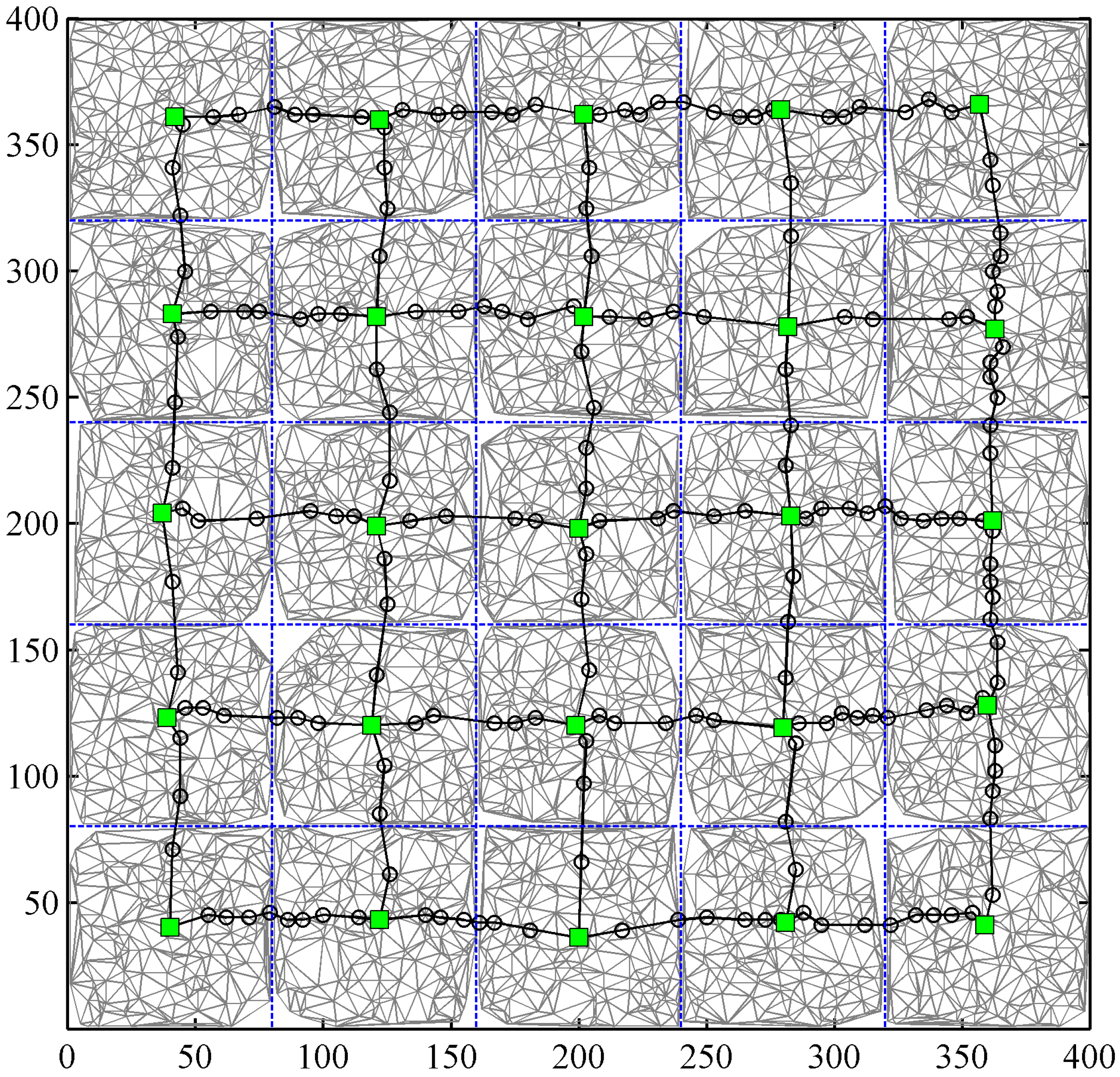
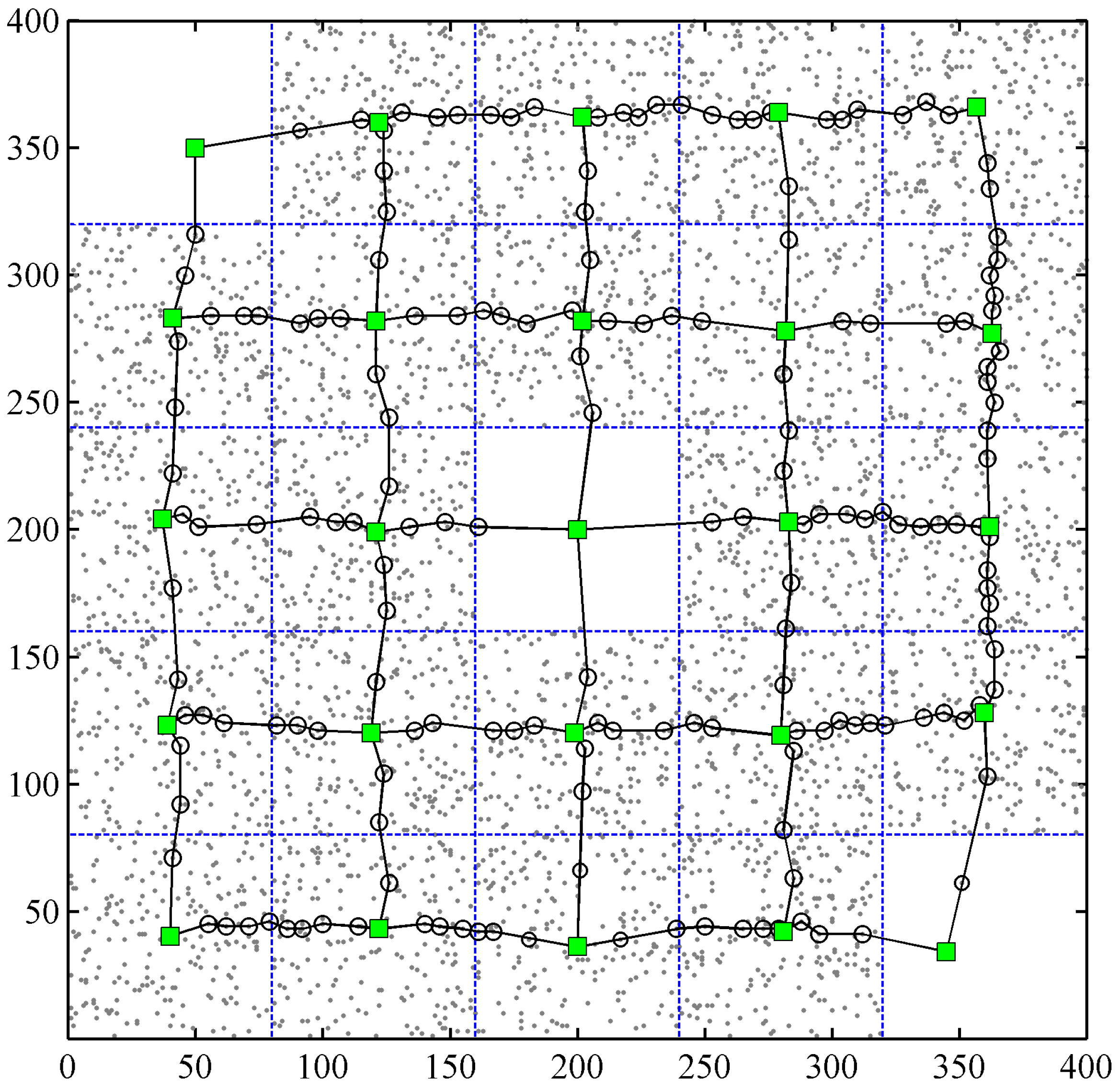
For better understanding, Figure 2 shows an example of gridding division of the 5000 PSs simulated for an area with a size of 400 × 400 pixels and the averaged PS density $\overline{\rho }$ of 1/32. If expecting the number N of PSs in each grid cell to be 100, one can simply infer by (1) that the grid size S should be of 6400 pixels, i.e., a square of 80 × 80 pixels. As shown in Figure 2, the imaged area is therefore divided into 5 × 5 grid cells.

Figure 2. An example of the global control network (GCN) and the localized triangular irregular networks (LTINs) constructed with the 5000 PSs (marked by dark dots) simulated for an area with a size of 400×400 pixels. A primary control point (PCP, marked by a filled green square) is selected for each grid, and the PCPs in adjacent grids are linked by the transition PCPs (marked by black circles), thus forming the GCN (marked by black lines). All the PSs in each grid are connected to form the LTIN (marked by gray lines).

Figure 2. An example of the global control network (GCN) and the localized triangular irregular networks (LTINs) constructed with the 5000 PSs (marked by dark dots) simulated for an area with a size of 400×400 pixels. A primary control point (PCP, marked by a filled green square) is selected for each grid, and the PCPs in adjacent grids are linked by the transition PCPs (marked by black circles), thus forming the GCN (marked by black lines). All the PSs in each grid are connected to form the LTIN (marked by gray lines).

2.2. Global Control Network Construction and Least Squares Solution

As mentioned previously, the two levels of PS networks, i.e., global control network (GCN) and localized triangular irregular network (LTIN), are constructed for estimating deformation rates. The former consists of the feature PSs selected from all the grid cells, while the latter consists of all the PSs in each grid cell. Such feature PSs are termed the primary control points (PCPs), which should be evenly distributed in the entire study area. Deformation rates at the PCPs can be estimated using LS adjustment.

2.2.1. Primary Control Point Selection and Global Control Network Construction

The PCPs are selected by considering two aspects, i.e., high SNR in phase measurements and proper location. For each grid cell, a representative PS is first selected as a core PCP that should have the smallest amplitude dispersion index [2] and the shortest distance to the center of the grid cell. The selection process for the core PCP can be represented by:

$$\text{Core PCP}\iff \text{minimize}\{AD{I}_i \times D_i\} i=1, 2, \mathrm{...}, n$$

(2)

where ADI_i stands for the amplitude dispersion index of the i^th PS (i = 1, 2, …, n) in the grid cell, n for the total number of PSs in the grid cell, and D_i for the distance between the grid center and the location of the i^th PS.

Considering that atmospheric delay varies quickly in space domain, the shorter distance between neighboring PCPs means a higher spatial correlation for neighborhood differential modeling. As the separation between two adjacent core PCPs is generally too large, we add some transition PCPs to shorten the distance.

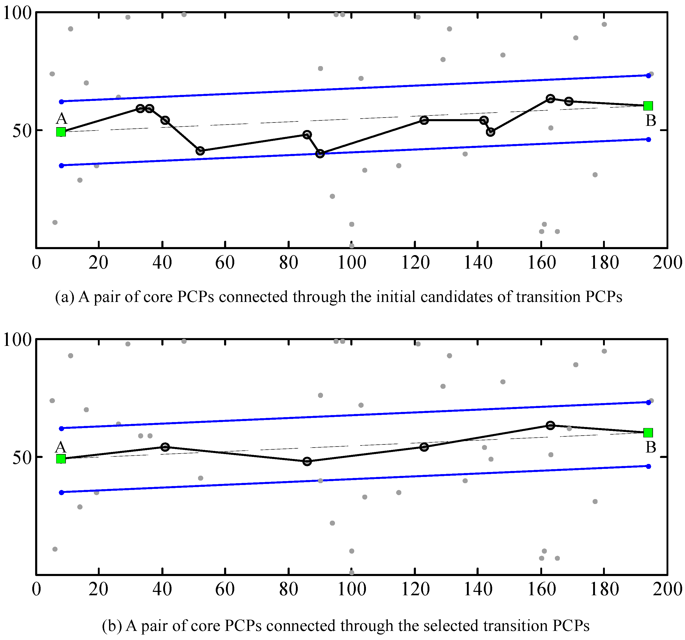
The transition PCPs should be determined using some definite criteria. Here we propose a two-step method for choosing the transition PCPs. As an example, Figure 3 shows how the transition PCPs between the two core PCPs (i.e., A and B) are identified properly. The first step is to set a boundary (i.e., blue lines in Figure 3) around the line AB (a band of 30 pixels used for this example), and the PSs within the boundary and located nearest to the line AB in each normal direction are chosen as the initial candidates of transition PCPs. The second step is to further discard some candidates through removing some very short arcs by using a distance threshold (30 pixels used for this example), thus obtaining the final transition PCPs. The points and connections derived by the two steps can be exemplified by Figure 3a and b, respectively. It can be seen from this example that four PSs are eventually selected as the transition PCPs from 11 PSs (i.e., the initial candidates for transition PCPs) through the two-step selection process.

It should be noted that there is only a core PCP for each grid (marked by a filled green square in Figure 2), and the transition PCPs (marked by black circles in Figure 2) between any two core PCPs from two adjacent grids should be identified using the procedures described above. Once both the core and transition PCPs are identified, they generally distribute along the longitudinal and transverse directions. We connect the two types of PCPs by minimizing the accumulative distance between adjacent PCPs, thus forming a grid-like network that is referred to as the GCN. As an example, Figure 2 shows the GCN constructed by using the core PCPs and transition PCPs selected from the simulated data. As a remark, special treatment should be given to the grids at the margin of the imaged area or other grids where only few PSs are available due to localized temporal decorrelation. If the total number of PSs in a grid is not greater than 4, all the PSs are chosen as the core or transition PCPs. If a grid is located at the image margin, the connections between the PCPs may be very weak (e.g., long arcs), thus resulting in some isolated arcs and PCPs. Therefore, we connect those PCPs to the core or transition PCPs in the adjacent grids, thus forming a closed path for further analysis. As an example, Figure 4 demonstrates such special treatment for constructing a GCN in the case of few PSs being available for some grids.

Figure 3. An example of the selection process of the transition primary control points (PCPs). The transition PCPs are selected from all the PSs located in the buffer defined by the blue lines around line AB, as shown in (a) to (b).

Figure 3. An example of the selection process of the transition primary control points (PCPs). The transition PCPs are selected from all the PSs located in the buffer defined by the blue lines around line AB, as shown in (a) to (b).

Figure 4. An example of global control network in the case of few PSs being available in several grids. Only one or two PSs are located in the top-left and bottom-right grid, respectively, and there is no PS in the central grid.

Figure 4. An example of global control network in the case of few PSs being available in several grids. Only one or two PSs are located in the top-left and bottom-right grid, respectively, and there is no PS in the central grid.

2.2.2. Least Squares Solution Based on the Global Control Network

For a PCP with pixel coordinates (x, y), the interferometric phase ${\text{Φ}}_i\left(x,t_i\right)$ in the i^th interferogram with temporal baseline t_i can be expressed by [2]:

$${\text{Φ}}_i(x,y;T_i)=\frac{4\text{π}}{\lambda \cdot R\cdot \text{sinθ}}\times B_i^{\perp }\times \text{ε}(x,y)+\frac{4\text{π}}{\lambda }\times T_i\times v(x,y)+{\varphi }_i^{res}(x,y;T_i)$$

(3)

where $B_i^{\perp }$ and T_i are the perpendicular (spatial) and temporal baselines, respectively; λ, R, and θ are the radar wavelength (3.1 cm for TSX case), the sensor-to-PCP distance, and the radar incidence angle, respectively; and $\text{ε}\left(x,y\right)$, $v\left(x,y\right)$, and ${\varphi }_i^{res}\left(x,y;T_i\right)$ are the elevation error, linear deformation rate along radar line of sight (LOS), and residual phase, respectively.

For an arc connecting two adjacent PCPs (l and p) in the GCN, the differential phase can be derived using Equation (3), i.e.,

$$\begin{array}{l}\text{Δ}{\text{Φ}}_i(x_l, y_l; x_p, y_p; T_i)=\frac{4\text{π}}{\lambda \cdot \overline{R}\cdot \text{sin}\overline{\text{θ}}}\times {\overline{B}}_i^{\perp }\times \text{Δε}(x_l, y_l; x_p, y_p)\\ +\frac{4\text{π}}{\lambda }\times T_i\times \text{Δ}v(x_l, y_l; x_p, y_p)+\text{Δ}{\varphi }_i^{res}(x_l, y_l; x_p, y_p; T_i)\end{array}$$

(4)

where ${\overline{B}}_i^{\perp }$, $\overline{R}$ and $\overline{\theta }$ are the mean perpendicular baseline, the mean sensor-to-PCP distance, and the mean incident angle of the two PCPs, respectively; and $\text{Δε}$ and $\text{Δ}v$ are the differential elevation error and the differential linear deformation rate between the two PCPs. With M interferograms generated from N SAR images, M observation equations as shown in Equation (4) can be obtained for any arc of the GCN.

By following the methodology proposed by Ferretti et al. [1,2], the unknowns $\text{Δε}$ and $\text{Δ}v$ of all the arcs in the GCN can be derived. Then, a LS solution can be applied to the GCN for the purpose of eliminating geometric inconsistency and deriving the most probable values for the deformation rate and elevation error for each PCP. For deformation rate estimation, the observation equation for the deformation rate increment between two adjacent PCPs is:

$${\widehat{v}}_p-{\widehat{v}}_l=\text{Δ}{v}_{pl}+r_{pl}, p\ne l, \forall p,l=1, 2, \dots , K$$

(5)

Where ${\widehat{v}}_l$ and ${\widehat{v}}_p$ are the deformation rates along radar LOS of the PCP l and PCP p, respectively; $\text{Δ}{v}_{pl}$ is the increment of deformation rates between the two PCPs; $r_{pl}$ is the residual of $\text{Δ}{v}_{pl}$; and K is the total number of PCPs in the GCN. The matrix form of the observation equations is written as:

$$\underset{Q\times K}{B}\times \underset{K\times 1}{X}=\underset{Q\times 1}{L}+\underset{Q\times 1}{R}$$

(6)

where B is a coefficient matrix; L and R are the vectors of the observations (i.e., deformation rate increments) and the residuals, respectively; Q is the total number of arcs in the GCN; and X is the vector of unknown deformation rates to be estimated, i.e.,

$$X=\left[\begin{array}{cccc}{\widehat{v}}_1,& {\widehat{v}}_2,& ...& {\widehat{v}}_K\end{array}\right]$$

(7)

Furthermore, let the weight matrix be

$$P=\left[\begin{array}{cccc}{\gamma }_1^2& 0& 0& 0\\ 0& {\gamma }_2^2& 0& 0\\ \text{M}& \text{M}& \text{M}& \text{M}\\ 0& 0& 0& {\gamma }_Q^2\end{array}\right]$$

(8)

whose diagonal elements are the squares of the model coherence (MC) values previously estimated for the PS pairs. Ferretti et al. indicate that if $\text{Δ}{\varphi }_i^{res}$ is small enough, say $\left|\text{Δ}{\varphi }_i^{res}\right|<\pi$, it is possible to estimate both $\text{Δε}$ and $\text{Δ}v$ directly from the M wrapped differential interferograms by maximizing the following objective function [1,2]:

$$\gamma =\left|\frac{1}{M}{\displaystyle \sum _{i=1}^M\left(\text{cos}\Delta {\omega }_i+j\times \text{sin}\Delta {\omega }_i\right)}\right|$$

(9)

where γ is the MC value of the two PS points; $j=\sqrt{-1}$, and $\text{Δ}{\omega }_i$ denotes the difference between the measured and the estimated phase values,

$$\Delta {\omega }_i=\Delta {\Phi }_i-\frac{4\pi }{\lambda \cdot \overline{R}\cdot \text{sin}\overline{\theta }}\times {\overline{B}}_i^{\perp }\times \text{Δ}\epsilon -\frac{4\pi }{\lambda }\times T_i\times \text{Δ}v$$

(10)

Therefore, the LS solution of the unknowns X can be expressed by:

$$X={(B^{T}PB)}^{-1}{B}^{T}PL$$

(11)

It should be noted that a reference point (e.g., a PCP without any movement or a leveling point with the known deformation rate) needs to be chosen for the LS solution, and the deformation rates of all other PCPs are derived relative to this reference point.

2.3. Localized Triangular Irregular Network Construction and Least Squares Solution

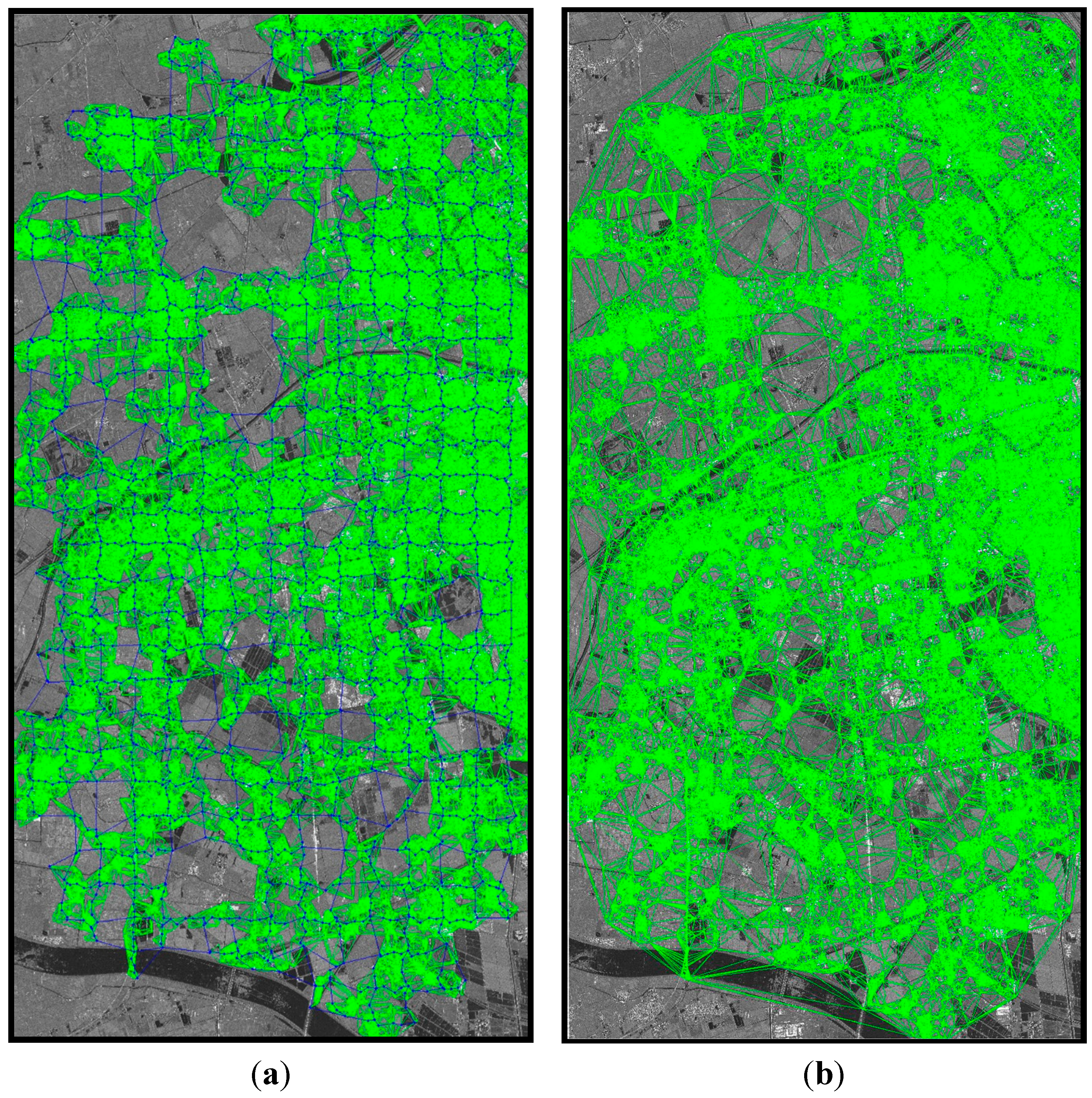
Upon completion of the first level networking and solution, the PCPs can be used as control points with the known deformation rates for the second-level analysis, which is performed on a grid-by-grid basis. For any grid cell, all the PSs (including the PCPs) are connected using the Delaunay triangulation method to form a localized triangular irregular network (LTIN). For the simulated data, Figure 2 also shows the resultant LTINs for all the grid cells and the associated GCN. It should be emphasized that each individual LTIN is related to the adjacent LTINs by the GCN, and considered as an individual processing unit. The estimation of deformation rates at the non-PCP PSs can be conducted by following the same procedures as described for the GCN-based LS solution in Section 2.2. The deformation rates at the PCPs derived by the first-level analysis are used as known data in the observation equations, thus providing the reference datum for the second level LS solution.

3. Study Area and Data Source

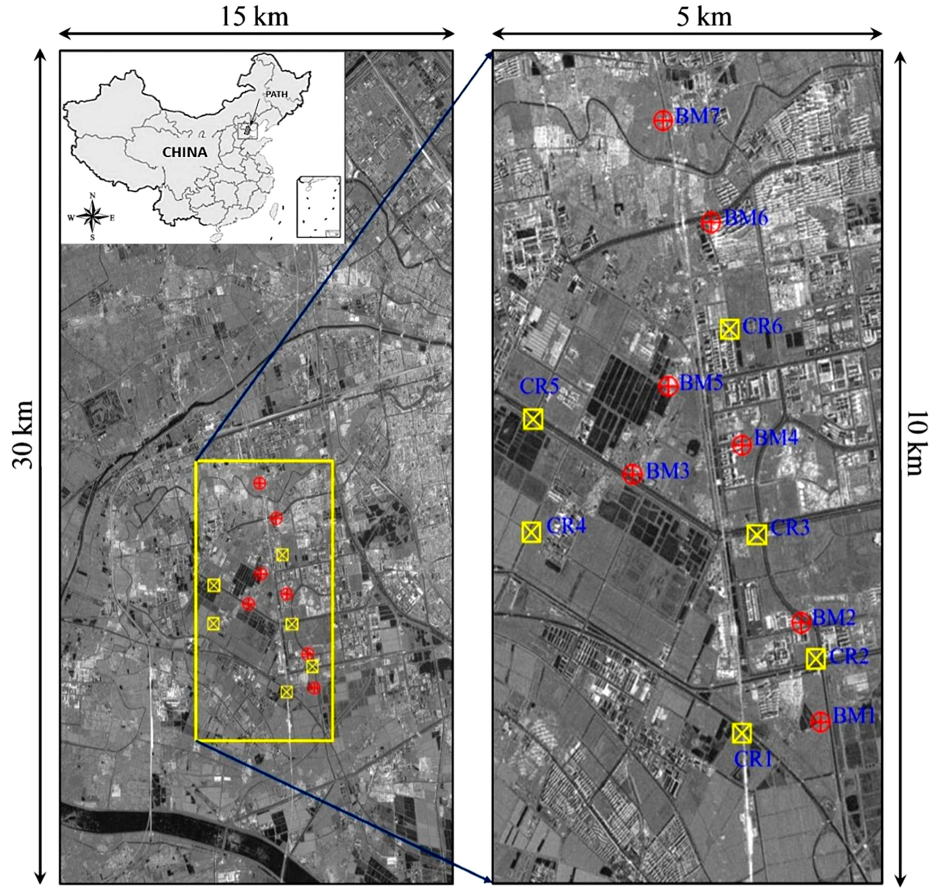
For validation purposes, we selected the northwestern part of Tianjin in China as the study area. As shown in Figure 5, the study area of 450 km² belongs to the alluvial plain of the Haihe River and has very flat relief with a relative elevation difference of 2–3 m [9]. As one of the biggest cities in China, Tianjin suffers water shortage due to its natural geographic condition and semi-arid climate [15]. To meet its industrial and agricultural needs, a large amount of groundwater has been exploited in Tianjin since the 1920s, thus resulting in severe land subsidence in many areas [16]. In recent years, some effective measures such as groundwater injection and restricting or prohibiting groundwater extraction in some planned zones have been taken to mitigate subsidence, and the subsidence rates in urban areas have slowed down to about 10–20 mm/year [17,18]. However, serious subsidence is still ongoing around suburban areas and reaches up to 100 mm/year due to overuse of groundwater [18,19].

Figure 5. The location map and the study area around Tianjin in China. The insert at the top-left corner shows the location map and the coverage of the TSX scenes. The left panel shows the amplitude image (averaged from 40 TSX images) in which the study area is marked by the rectangle. The right panel shows the enlarged amplitude image of the study area in which the seven benchmarks (BMs) and six corner reflectors (CRs) are annotated for later analysis.

Figure 5. The location map and the study area around Tianjin in China. The insert at the top-left corner shows the location map and the coverage of the TSX scenes. The left panel shows the amplitude image (averaged from 40 TSX images) in which the study area is marked by the rectangle. The right panel shows the enlarged amplitude image of the study area in which the seven benchmarks (BMs) and six corner reflectors (CRs) are annotated for later analysis.

For subsidence extraction, we used 40 TSX images acquired by SpotLight mode along descending orbits between 27 March 2009 and 25 December 2010 (all imaging at 6:17 am local time with pixel spacing of 1.36 m in slant range and 1.90 m in azimuth). The 376 interferometric pairs were generated by setting the spatial baseline threshold to 120 m. Although the study area is flat, the SRTM DEM with a spacing of 3 arc sec was used to remove topographic effects from all 376 interferograms. As seen in Figure 5, the seven BMs and six CRs were used for verification purpose. The four epochs of second-order leveling campaigns (with accuracy of 2 mm/km in height difference) were conducted on both the BMs and the CRs during the period of the TSX acquisitions. The leveling dates for the four epochs are around 20 April 2009, 5 September 2009, 15 April 2010, and 30 October 2010, respectively.

4. Experimental Results and Analysis

4.1. The Global Control Network and Localized Triangular Irregular Networks Constructed

The PSs in this study area were screened out using the 40 TSX amplitude images through statistical calculation of ADI on a pixel-by-pixel basis [8]. Any pixel with an ADI value less than 0.25 is identified as a PS. Then, 1,004,024 PSs were selected from the study area of 450 km² that was imaged with 7500 and 15,000 pixels in slant range and azimuth, respectively. The averaged density of the PSs in the entire study area is 2230 per square kilometer. The gridding division of the identified PSs was then performed by letting the expected number of PSs in each grid cell be about 2300. With N = 2300 and $\overline{\rho }$ = 1/112, we can deduce that the grid size S ≈ 250,000. This means that the grid size should be 500 × 500 pixels (i.e., corresponding to about 1 km² for the TSX case), thus resulting in 15 × 30 grid cells for the study area. Based on further analysis, the selected PSs are distributed among 404 grid cells, and the remaining 46 grid cells do not have PSs due to serious temporal decorrelation in farming lands.

By following the procedures as described for PCP selection and GCN construction in Section 2.2, 404 core PCPs and 952 transition PCPs were identified. For selecting the transition PCPs between two adjacent core PCPs, we used a band of 60 pixels (i.e., an interval of about 120 m) for choosing the initial candidates and a threshold of 25 pixels (i.e., 50 m) for removing the short arcs. As shown in Figure 6a, the GCN and the multiple LTINs can be constructed by following the procedures as described above. As shown in Figure 6b, we also constructed a global TIN for later comparison analysis. There are 2832 arcs in the GCN, and 2,998,810 arcs in all the LTINs (including 1,995,195 triangles), while there are 3,011,804 arcs in the global TIN (including 2,007,781 triangles).

4.2. Subsidence Rates and Evaluation

4.2.1. Subsidence Rates at Persistent Scatterers

Figure 7 shows the subsidence rates at all the PSs estimated through the hierarchical approach of networking and solution in the study area. To derive a unique solution, we took the BM3 as a reference point for the LS-based adjustment, whose subsidence rate was calculated using the four epochs of leveling measurements. For comparison purposes, we also carried out a solution for the global TIN as shown in Figure 6b, thus obtaining another set of subsidence rates at all the PSs.

Figure 6. The two types of PS networking for the study area: The left panel (a) shows the global control network (GCN) plus localized triangular irregular networks (LTINs) in the 15 × 30 grids of the study area, including 2832 arcs in the GCN and 2998810 arcs in the LTINs. The right panel (b) shows the global triangular irregular network (TIN) of the study area, including 3011804 arcs.

Figure 6. The two types of PS networking for the study area: The left panel (a) shows the global control network (GCN) plus localized triangular irregular networks (LTINs) in the 15 × 30 grids of the study area, including 2832 arcs in the GCN and 2998810 arcs in the LTINs. The right panel (b) shows the global triangular irregular network (TIN) of the study area, including 3011804 arcs.

As seen in Figure 7, the subsidence rates derived by the hierarchical approach in the entire study area range between 0 and 110 mm/year, and exhibit an uneven distribution. Although the subsidence rates range between 0 and 20 mm/year in the main urbanized areas (i.e., the east side in Figure 7), the subsidence rates in the suburban areas are obviously higher. As indicated by ovals (i.e., A, B, C, and D) in Figure 7, four remarkable subsidence troughs appear in the suburban areas, whose maximum subsidence rates reach up to 75, 68, 52, and 110 mm/year, corresponding to Shuangjie, Qingguang, Shanghetou, and Jingwu towns, respectively. This confirms that the subsidence rates in the downtown areas have been slowed down due to the reduction of groundwater extraction that has been executed in Tianjin as a municipal management action in recent years [15,16,17,18]. However, remarkable land subsidence has taken place in the suburban areas due to increasing extraction of groundwater primarily for agricultural production [19].

Figure 7. The subsidence rates at all the PSs derived by the proposed hierarchical approach. Four remarkable subsidence troughs appeared in the suburban areas, as marked by ovals (i.e., A, B, C, and D), corresponding to Shuangjie, Qingguang, Shanghetou, and Jingwu towns, respectively.

Figure 7. The subsidence rates at all the PSs derived by the proposed hierarchical approach. Four remarkable subsidence troughs appeared in the suburban areas, as marked by ovals (i.e., A, B, C, and D), corresponding to Shuangjie, Qingguang, Shanghetou, and Jingwu towns, respectively.

4.2.2. Quality Assessment and Uncertainty Analysis

By statistical calculation, we analyzed the differences of subsidence rates between the two types of solutions (i.e., based on the GCN-LTINs and the global TIN). Figure 8 shows the discrepancies at all the PSs. It can be concluded that the two types of solution are globally in close agreement with each other. However, a closer inspection of Figure 8 indicates that some minor jumps in the discrepancies appear in the image space.

Figure 8. The distribution of discrepancies of subsidence rates at all the PSs between two types of solutions based on the global control network plus localized triangular irregular networks and the global triangular irregular network, respectively.

Figure 8. The distribution of discrepancies of subsidence rates at all the PSs between two types of solutions based on the global control network plus localized triangular irregular networks and the global triangular irregular network, respectively.

Figure 9 shows the histogram of the discrepancies between the subsidence rates derived from the two types of solutions. It can be observed that the discrepancies range between −2.5 and 1.9 mm/year, and approximately follow the normal distribution. The mean and the root mean squared error (RMSE) of the discrepancies are −0.04 and ±0.74 mm/yr, respectively. This means that the subsidence rates derived from the global TIN evolve more smoothly in space than those derived from the GCN-LTINs. It can be understood that more connections in the global TIN are advantageous in smoothing the subsidence rates derived from the LS-based solution. The relatively weak connections in the GCN may cause slight jumps in the subsidence rates between neighboring grids, although the resultant errors are negligible for this study. Further investigation will be performed in our future work to overcome such drawbacks.

Figure 9. The histogram of discrepancies of subsidence rates at all the PSs between two types of solutions based on the global control network plus localized triangular irregular networks and the global triangular irregular network, respectively.

Figure 9. The histogram of discrepancies of subsidence rates at all the PSs between two types of solutions based on the global control network plus localized triangular irregular networks and the global triangular irregular network, respectively.

For validation purposes, we utilized the leveling measurements at BM1–BM7 and CR1–CR6 as the reference data to analyze the quality of subsidence time series derived from the two types of PSI solutions based on the GCN-LTINs and the global TIN, respectively. The comparison analysis on subsidence rates at all the checkpoints shows that the mean and RMSE of discrepancies between the leveling and the GCN-LTINs PSI solution are 0.7 mm/year and ±2.4 mm/year, respectively, while the mean and RMSE related to the global-TIN PSI solution are 0.7 mm/year and ±2.3 mm/year, respectively. Moreover, the statistical calculation shows that the RMSEs between subsidence values derived from leveling data and the GCN-LTINs PSI solution at all the checkpoints are ±2.0, ±3.4, and ±3.4 mm, respectively, for the three consecutive time spans (i.e., April to September of 2009, September of 2009 to April of 2010, and April to October of 2010), while the RMSEs related to the global-TIN PSI solution are ±2.2, ±3.3, and ±3.1 mm, respectively. For the entire time span, the RMSEs related to the GCN-LTINs and global-TIN PSI solution are ±2.5 and ±2.4 mm, respectively. This means that the subsidence time series derived from the hierarchical (i.e., GCN-LTINs) PSI solution is in good agreement with the leveling measurements and those derived from the global-TIN PSI solution. This indicates that the algorithm proposed in this paper is useful for extracting deformation time series.

4.2.3. Analysis of Computational Efficiency

For further analysis of computational efficiency, the computer time and memory used were recorded for the two types of LS-based PSI solutions in the study area, i.e., the GCN-LTINs- and global-TIN-based solutions. All the data reduction procedures were performed using the same desktop computer. Based on the system record, Table 1 lists the comparison of data quantity (i.e., total arcs), computing time, and memory used for the two types of PSI solutions. Although the total number of arcs in the GCN-LTINs is similar to that in the global TIN, a 78% time decrease and 95% memory reduction have been achieved by using the hierarchical approach for estimating the subsidence rates in the study area when compared to the global-TIN-based method. As the computation cost for the LS solution increases exponentially with an increase in the number of unknown parameters to be estimated (see Equation (11)), the dividing and conquering method with the GCN-LTINs can significantly decrease the computation cost.

It also should be emphasized that computer memory overflow issues can be generally avoided by using the two levels of PS network construction and solution. Therefore, the hierarchical approach proposed in this paper is very suitable for estimating deformation rates even over a huge area of interest with the use of time series of high-resolution SAR images. Moreover, the reduction of computer time for the PSI solution will play a crucial role when dealing with emergency situations [20].

Table 1. Comparison of computing time and memory required for the two types of solutions based on the global control network plus localized triangular irregular networks and the global triangular irregular network, respectively.

Method of PS Networking	Global TIN	GCN-LTINs
		GCN	LTINs
Total arcs	3011804	2832	2998810 [7, 48,473] × 404
Computer time used	98.6 min	3.7 s	21.6 min [0.01, 18.6] s × 404
Computer memory used	30.2 GB	128 MB	<1.4 GB

Table 1. Comparison of computing time and memory required for the two types of solutions based on the global control network plus localized triangular irregular networks and the global triangular irregular network, respectively.

Method of PS Networking	Global TIN	GCN-LTINs
		GCN	LTINs
Total arcs	3011804	2832	2998810 [7, 48,473] × 404
Computer time used	98.6 min	3.7 s	21.6 min [0.01, 18.6] s × 404
Computer memory used	30.2 GB	128 MB	<1.4 GB

Although the computation cost has been estimated only with the single thread operation, the hierarchical approach proposed in this paper can be extended to the parallel computation, thus leaving room for future work. In addition, we believe that the hierarchical approach has great potential for dealing with other high-resolution SAR images acquired by the new sensors, such as C-band Sentinel and L-band ALOS/PALSAR-2.

5. Conclusions

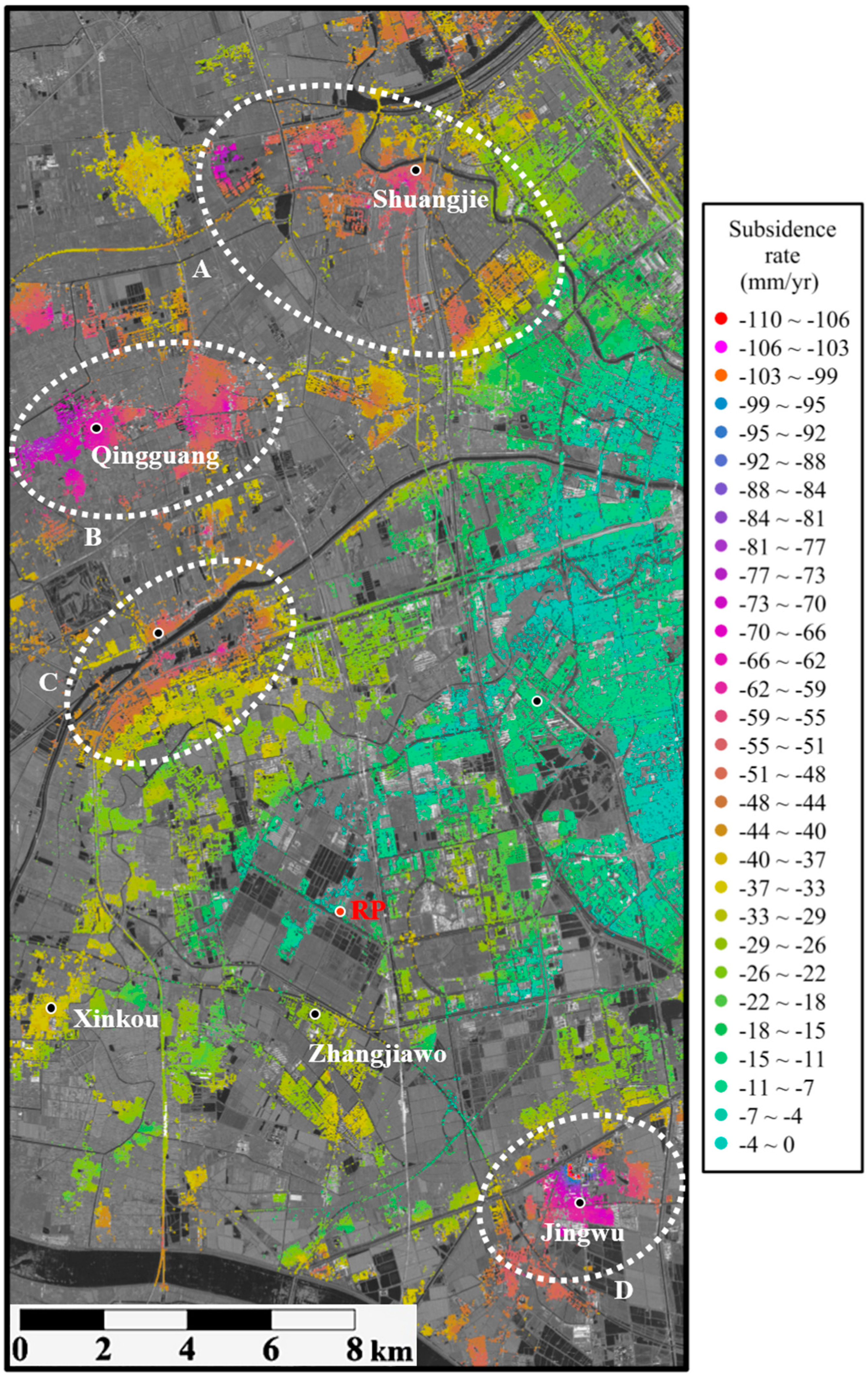
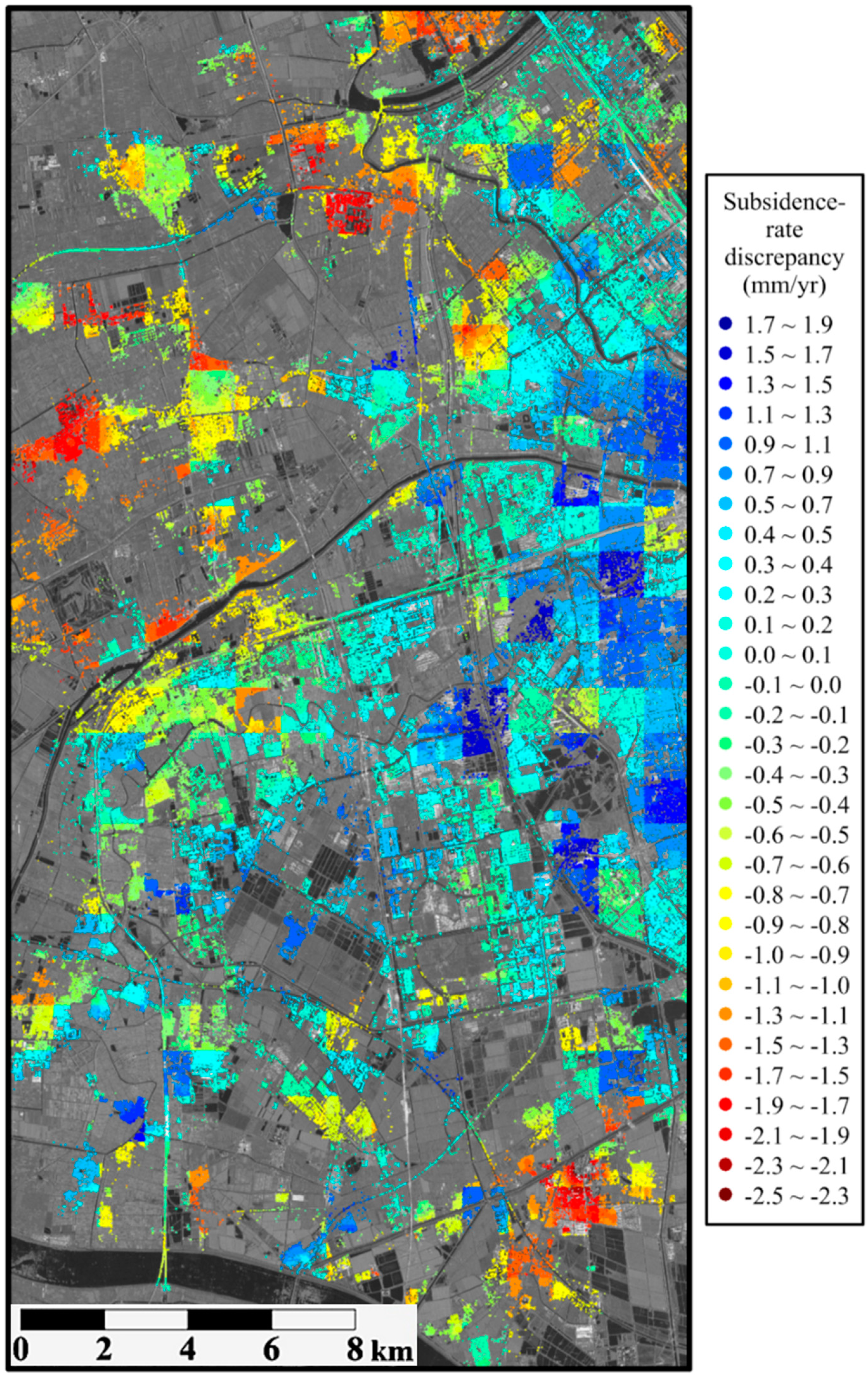
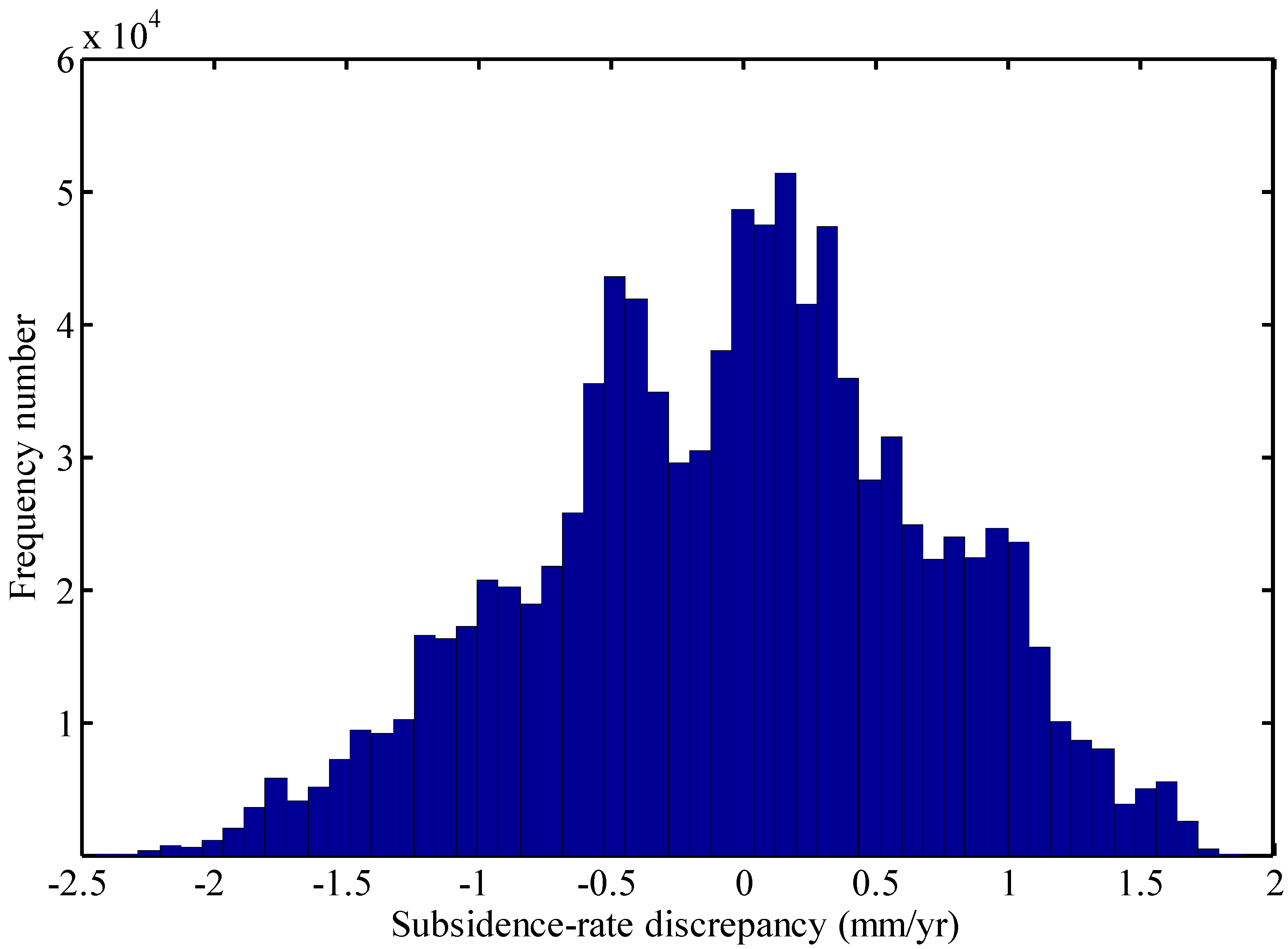
For the purpose of balancing between computational efficiency and solution accuracy, this paper presents a hierarchical approach in PSI, i.e., two levels of PS networking and solution, for estimating deformation rates with time series of high-resolution satellite SAR images. For validation purposes, the algorithm was tested using 40 high-resolution TSX images collected by SpotLight mode between 2009 and 2010 over Tianjin in China. The subsidence rates estimated by the hierarchical solution varied between 0 and 110 mm/year in the study area of 450 km². The subsidence rates in the suburban areas range between 30 and 110 mm/year, which are higher than those (0 to 20 mm/year) in the urban areas. This confirms that subsidence due to ground water extraction is still severe in the suburban areas.

The subsidence rates derived by the leveling and the hierarchical (i.e., GCN-LTINs) PSI solution are comparable at seven BMs and six CRs, and the mean and RMSE of their discrepancies are 0.7 mm/year and ±2.4 mm/year, respectively. The subsidence time series derived from the hierarchical PSI solution is in good agreement with the leveling measurements and those derived from the global-TIN PSI solution. Moreover, the hierarchical method for estimating subsidence rates in the study area raises the computational efficiency and reduces the memory consumption if compared with the method based on the global TIN. It can be concluded that the hierarchical approach proposed in this paper is very suitable for estimating deformation rates even over a huge area with time series of high-resolution SAR images.

It should be pointed out that the relatively weak connections in the GCN used in this study may cause slight jumps in the subsidence rates between neighboring grids. Although the resultant errors are negligible for this study, further investigation should be performed to overcome such drawbacks in the hierarchical approach, thus leaving room for future work.