
Deriving Snow Cover Metrics for Alaska from MODIS


Abstract
:
1. Introduction
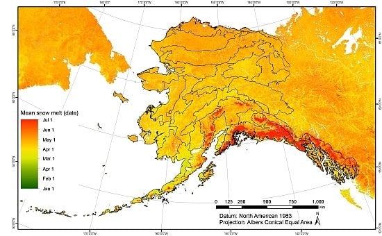
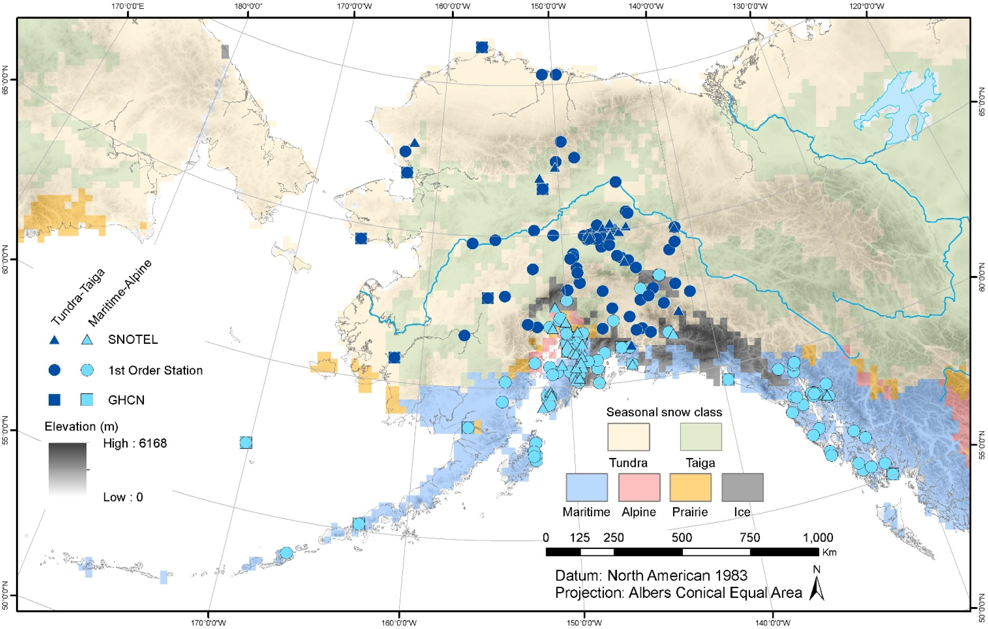
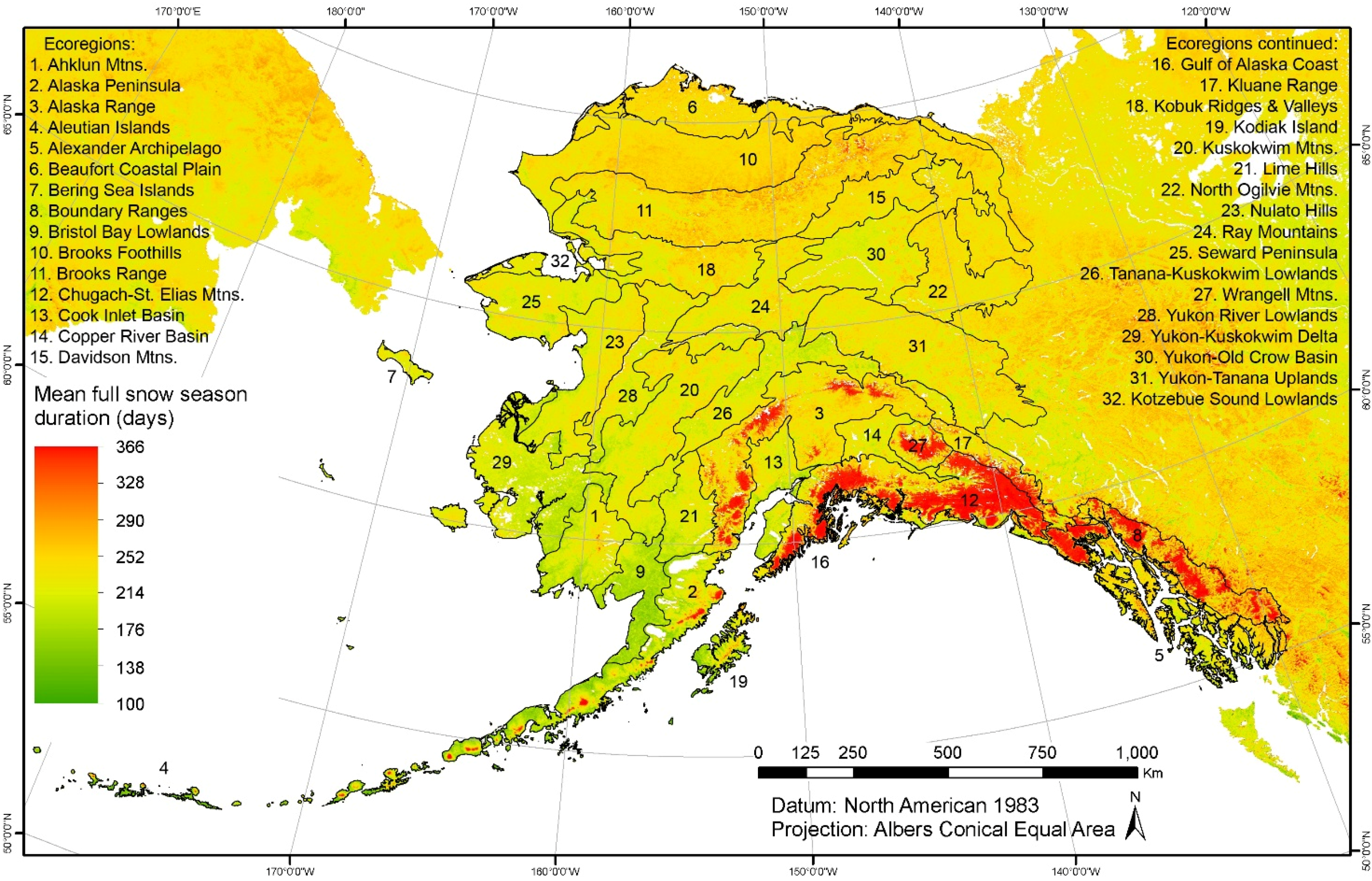
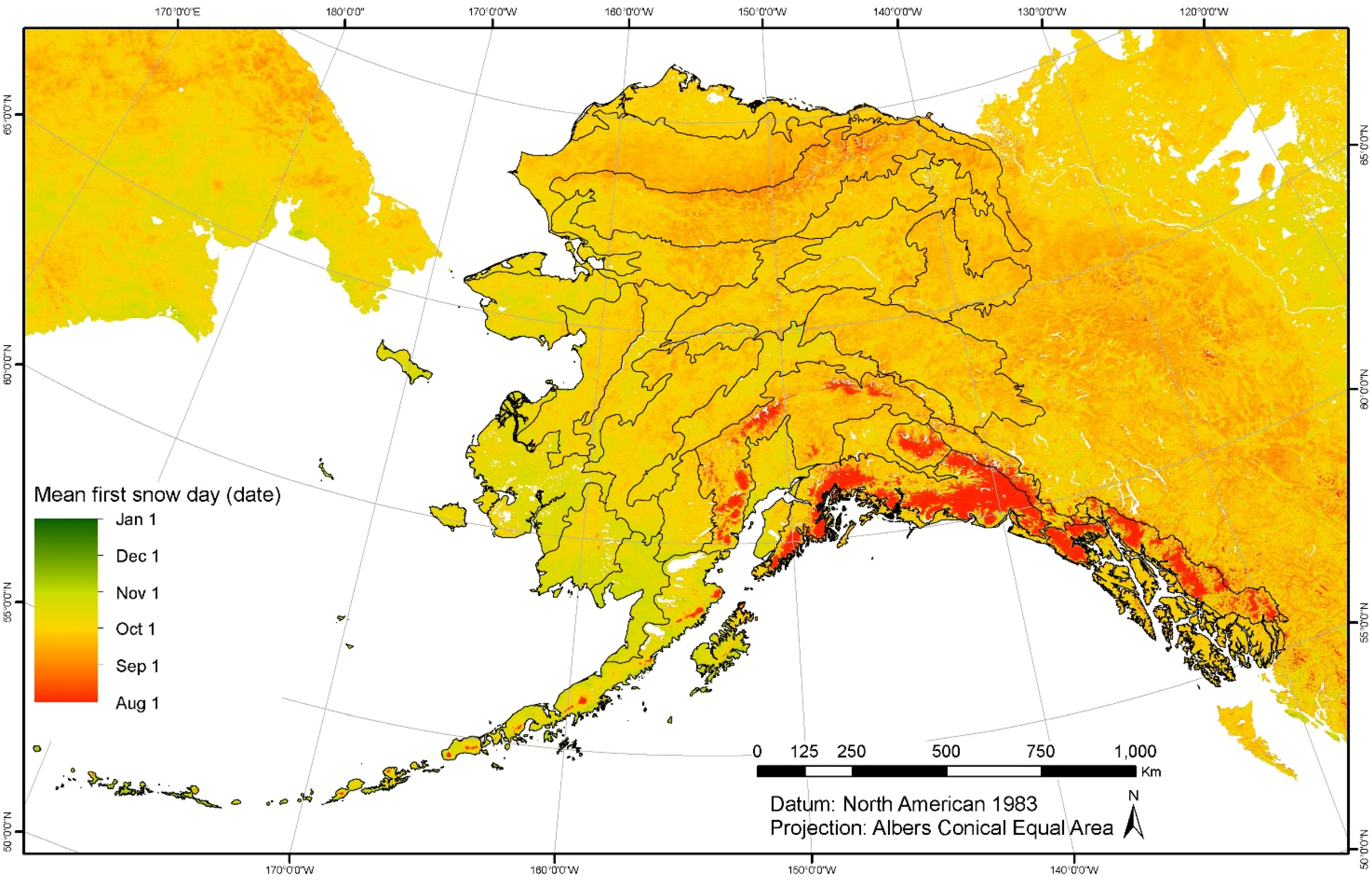
1.1. Study Area

2. Methods
2.1. Satellite and In Situ Data
2.1.1. MODIS Snow Product
2.1.2. In Situ Snow Onset and Snow Melt Dates
2.2. Filtering Algorithm
2.2.1. Spatial Filtering
2.2.2. Temporal Filtering
2.2.3. Snow Cycle Filtering
2.2.4. Reclassification of Permanent Snow and Ice
2.3. Snow Metrics
2.3.1. Definitions and Calculations

| Metrics Band Name | Metrics Description | Acronym | GeoTIFF Band |
|---|---|---|---|
| first_snow_day * | First snow day of the full snow season | FSD | 1 |
| last_snow_day * | Last snow day of the full snow season | LSD | 2 |
| first_last_snow_day_range | Duration of the full snow season | FLSDR | 3 |
| longest_css_first_day * | First snow day of the longest continuous snow season | LCFD | 4 |
| longest_css_last_day * | Last day of the longest continuous snow season | LCLD | 5 |
| longest_css_day_range | Duration of the longest continuous snow season | LCDR | 6 |
| snow_days | Number of days classified as snow after filtering | SD | 7 |
| no_snow_days | Number of days not classified as snow after filtering | NSD | 8 |
| css_segment_num | Number of segments within continuous snow season | CSN | 9 |
| mflag | Overall surface condition and snow-cover character for pixel | 10 | |
| cloud_days | Number of days classified as cloud after filtering | CD | 11 |
| tot_css_days | Total number of days within all continuous snow season segments | TCD | 12 |
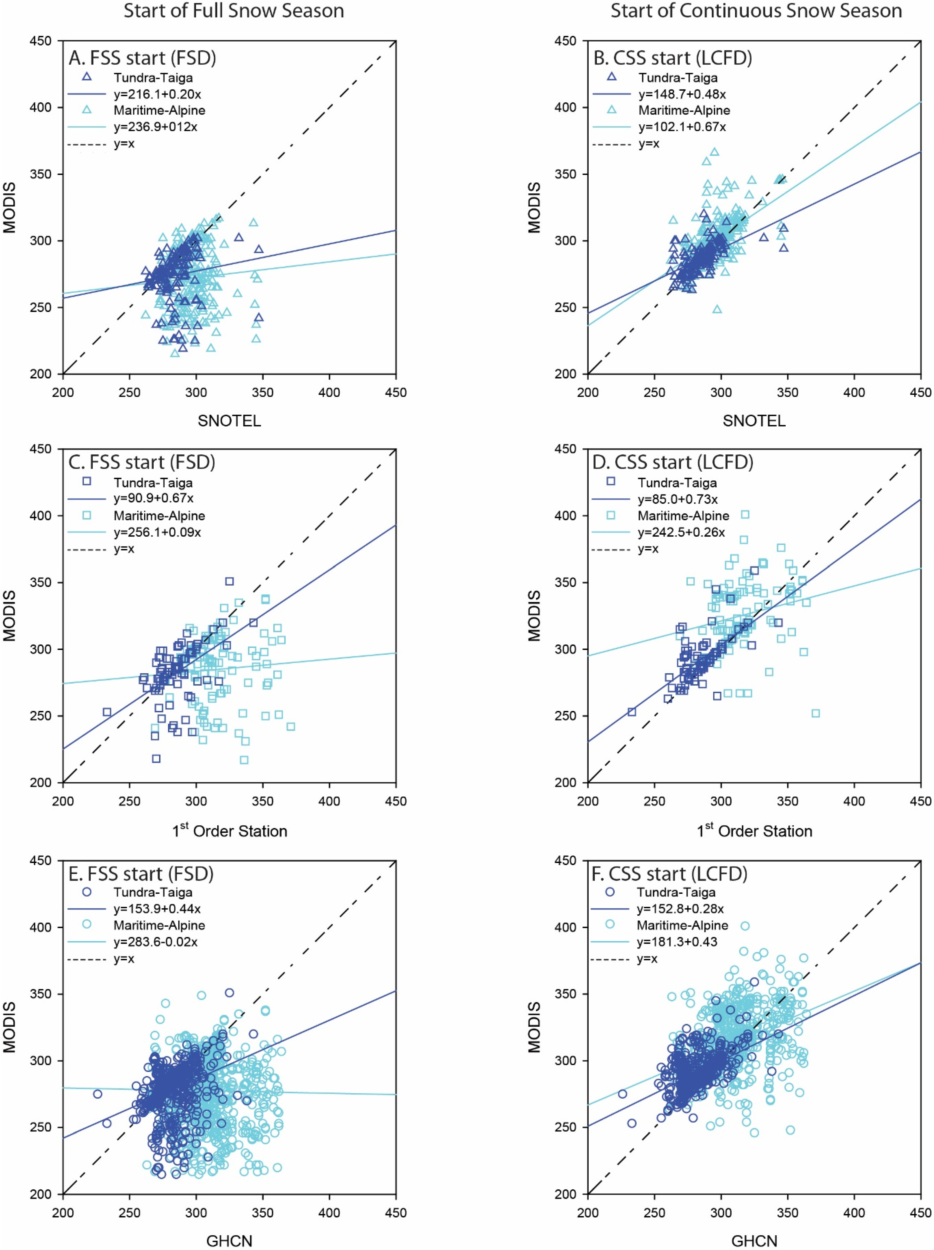
2.3.2. Accuracy Assessment
3. Results and Discussion
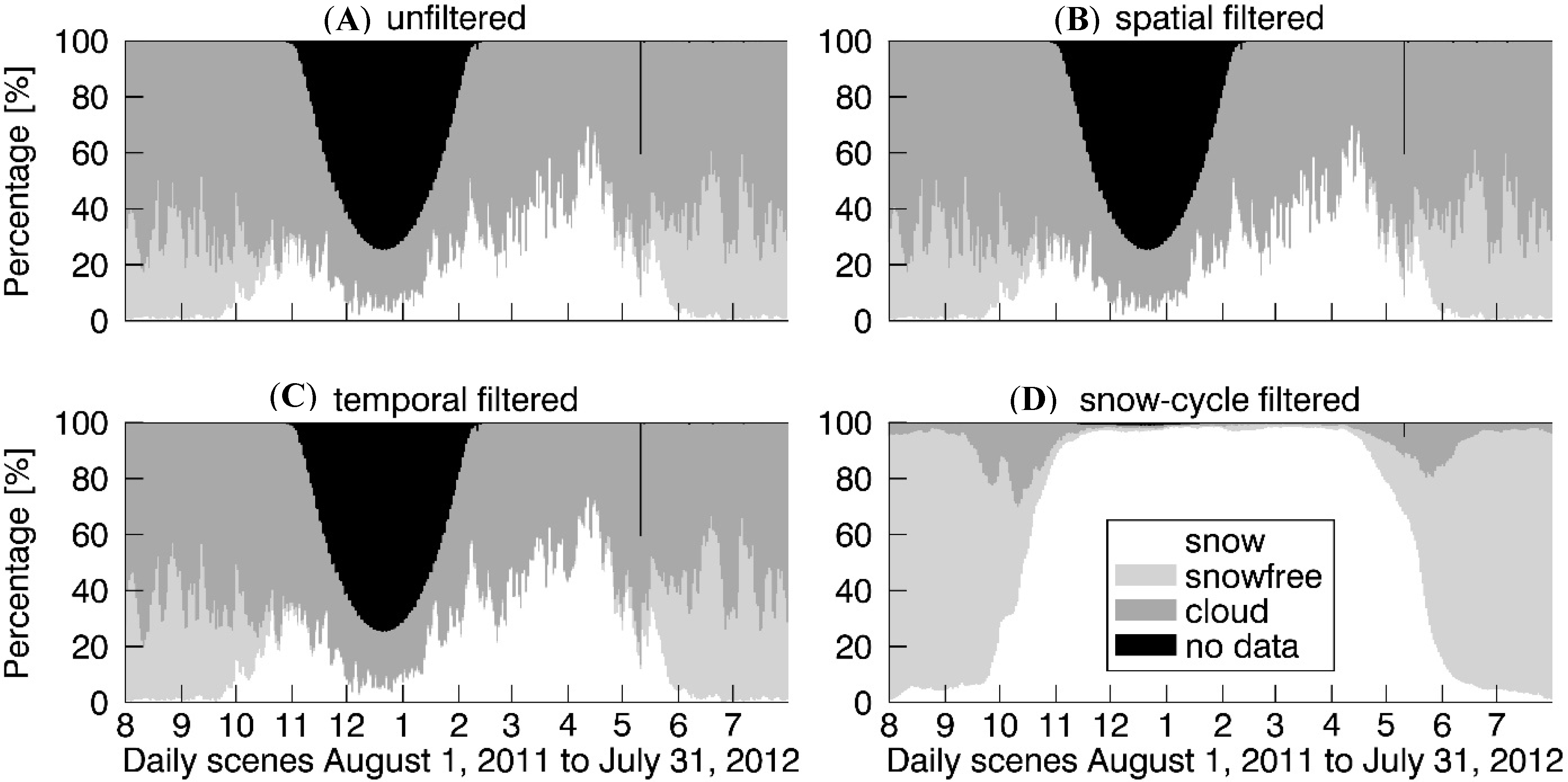
3.1. Effectiveness of Cloud-Filling Procedures

| Pixel Type | Filtering Step | Min (%) | Lower Quartile (%) | Median (%) | Upper Quartile (%) | Max (%) | Pixels (Nobs) | Pixels (%) | Change (%) |
|---|---|---|---|---|---|---|---|---|---|
| Cloud | No filter | 15.9 | 47.2 | 60.8 | 70.1 | 83.8 | 3,135,933,945 | 27.7 | |
| Spatial | 15.9 | 46.8 | 59.9 | 69.5 | 83.1 | 3,107,994,184 | 27.5 | −0.2 | |
| Temporal | 14.0 | 39.9 | 54.0 | 64.3 | 79.2 | 2,836,469,457 | 25.1 | −2.6 | |
| Snow cycle | 0.18 | 0.74 | 2.39 | 6.38 | 29.9 | 346,893,903 | 3.1 | −24.6 | |
| No data | No filter | 0.35 | 0.37 | 0.39 | 8.14 | 74.9 | 6,529,890,453 | 57.7 | |
| Spatial | 0.35 | 0.37 | 0.39 | 8.14 | 74.9 | 6,529,890,453 | 57.7 | 0.0 | |
| Temporal | 0.35 | 0.37 | 0.39 | 8.14 | 74.9 | 6,529,890,453 | 57.7 | 0.0 | |
| Snow cycle | 0.34 | 0.34 | 0.35 | 0.39 | 5.33 | 5,818,261,223 | 51.5 | −6.2 | |
| Snow | No filter | 0.31 | 1.76 | 11.7 | 27.4 | 69.0 | 899,588,089 | 8.0 | |
| Spatial | 0.31 | 1.76 | 11.8 | 27.9 | 69.4 | 917,672,537 | 8.1 | 0.1 | |
| Temporal | 0.32 | 1.84 | 13.2 | 32.4 | 72.9 | 1,067,052,916 | 9.4 | 1.4 | |
| Snow cycle | 0.66 | 6.41 | 82.1 | 97.3 | 98.7 | 3,196,893,025 | 28.3 | 20.3 | |
| Snow free | No filter | 0.10 | 0.63 | 3.70 | 26.7 | 58.9 | 742,185,329 | 6.6 | |
| Spatial | 0.10 | 0.63 | 3.70 | 27.0 | 59.4 | 752,040,642 | 6.7 | 0.1 | |
| Temporal | 0.12 | 0.68 | 4.27 | 31.5 | 65.1 | 874,184,990 | 7.7 | 1.1 | |
| Snow cycle | 0.23 | 1.14 | 9.38 | 87.3 | 95.5 | 1,945,549,665 | 17.2 | 10.6 |
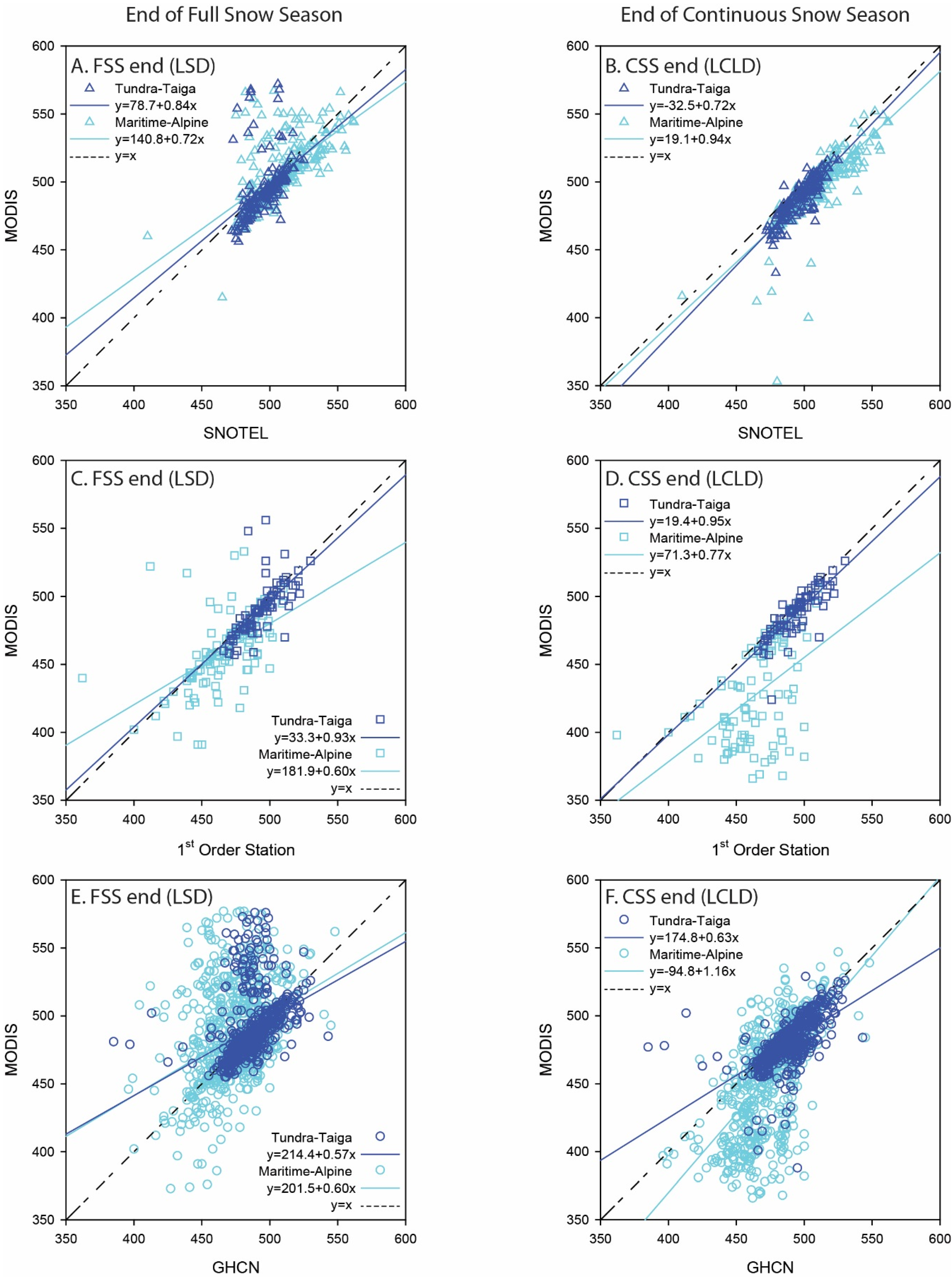
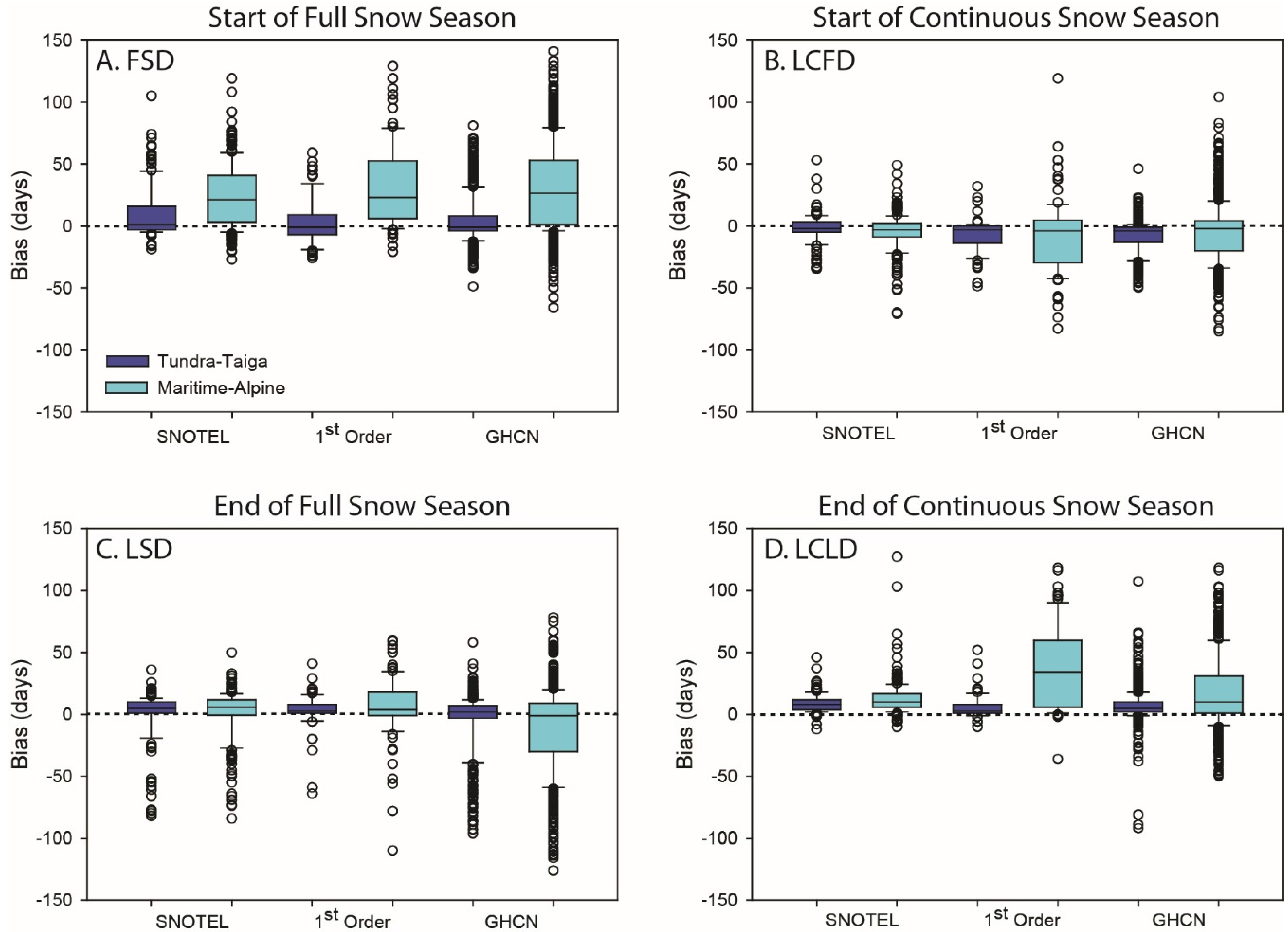
3.2. Accuracy Assessment
| Metric | Station Type | Snow Class | Number Obs. | RMSE (days) | Modeled Mean Bias (days) | SE(days) | r |
|---|---|---|---|---|---|---|---|
| FSD | SNOTEL | Tundra/Taiga | 147 | 23.4 | 11.2 | 2.4 | 0.15 |
| Maritime/Alpine | 223 | 35.5 | 22.0 | 1.8 | 0.02 | ||
| 1st Order | Tundra/Taiga | 79 | 19.3 | 0.7 | 3.3 | 0.51 | |
| Maritime/Alpine | 105 | 45.0 | 30.0 | 3.0 | 0.79 | ||
| GHCN | Tundra/Taiga | 592 | 19.1 | 6.1 | 1.4 | 0.33 | |
| Maritime/Alpine | 724 | 45.5 | 25.3 | 1.1 | −0.01 | ||
| LCFD | SNOTEL | Tundra/Taiga | 147 | 11.4 | −2.6 | 1.7 | 0.58 |
| Maritime/Alpine | 223 | 15.5 | −5.1 | 1.3 | 0.64 | ||
| 1st Order | Tundra/Taiga | 78 | 15.7 | −12.2 | 2.3 | 0.67 | |
| Maritime/Alpine | 104 | 30.4 | −4.1 | 2.2 | 0.72 | ||
| GHCN | Tundra/Taiga | 588 | 15.1 | −10.2 | 1.0 | 0.70 | |
| Maritime/Alpine | 716 | 23.7 | −4.6 | 0.8 | 0.44 | ||
| LSD | SNOTEL | Tundra/Taiga | 149 | 20.1 | 3.9 | 2.3 | 0.45 |
| Maritime/Alpine | 225 | 19.6 | 1.3 | 1.8 | 0.63 | ||
| 1st Order | Tundra/Taiga | 77 | 14.5 | 5.7 | 3.2 | 0.69 | |
| Maritime/Alpine | 104 | 26.0 | 8.3 | 3.0 | 0.85 | ||
| GHCN | Tundra/Taiga | 589 | 23.0 | −4.7 | 1.4 | 0.34 | |
| Maritime/Alpine | 737 | 34.7 | −5.7 | 1.0 | 0.37 | ||
| LCLD | SNOTEL | Tundra/Taiga | 149 | 11.5 | 9.7 | 2.0 | 0.87 |
| Maritime/Alpine | 225 | 19.1 | 33.9 | 2.5 | 0.89 | ||
| 1st Order | Tundra/Taiga | 77 | 11.1 | 9.0 | 2.7 | 0.83 | |
| Maritime/Alpine | 99 | 49.4 | 33.9 | 2.5 | 0.94 | ||
| GHCN | Tundra/Taiga | 590 | 15.0 | 9.0 | 1.1 | 0.55 | |
| Maritime/Alpine | 713 | 32.9 | 16.1 | 0.9 | 0.69 |


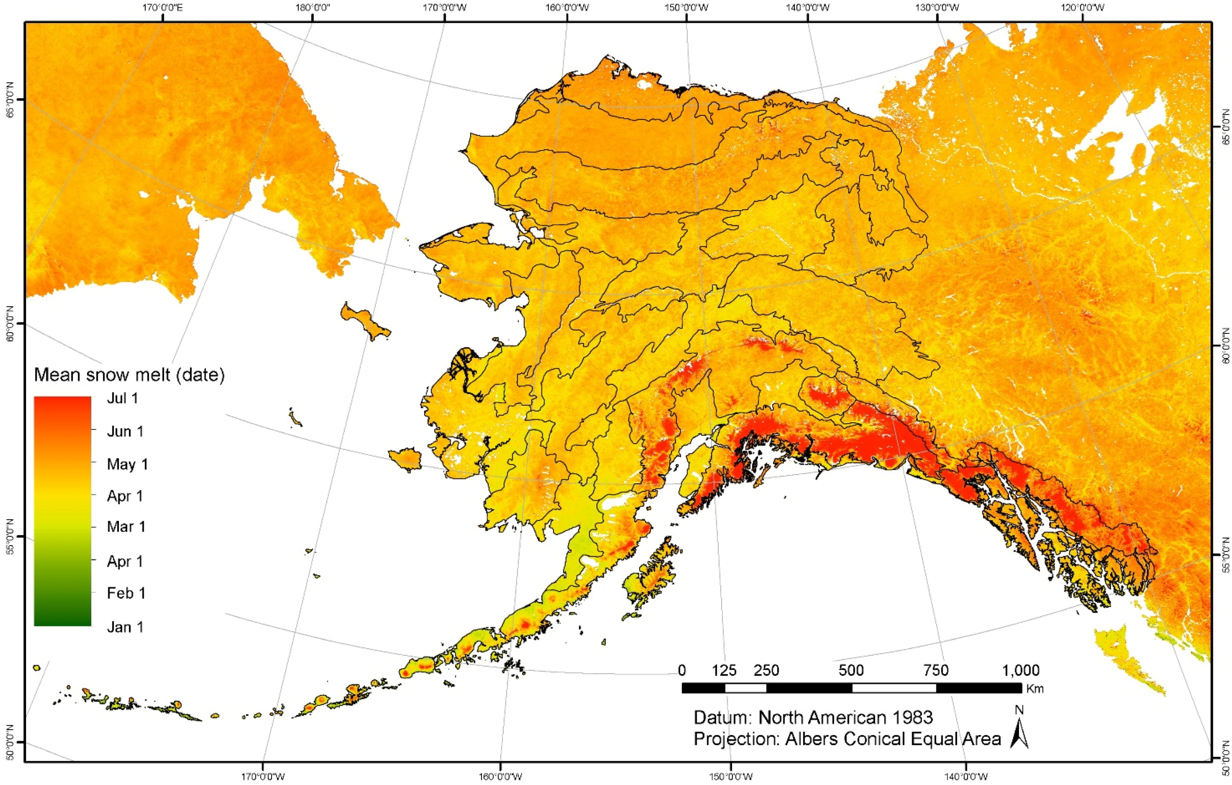
3.3. Snow Metrics
3.3.1. Full Snow Season


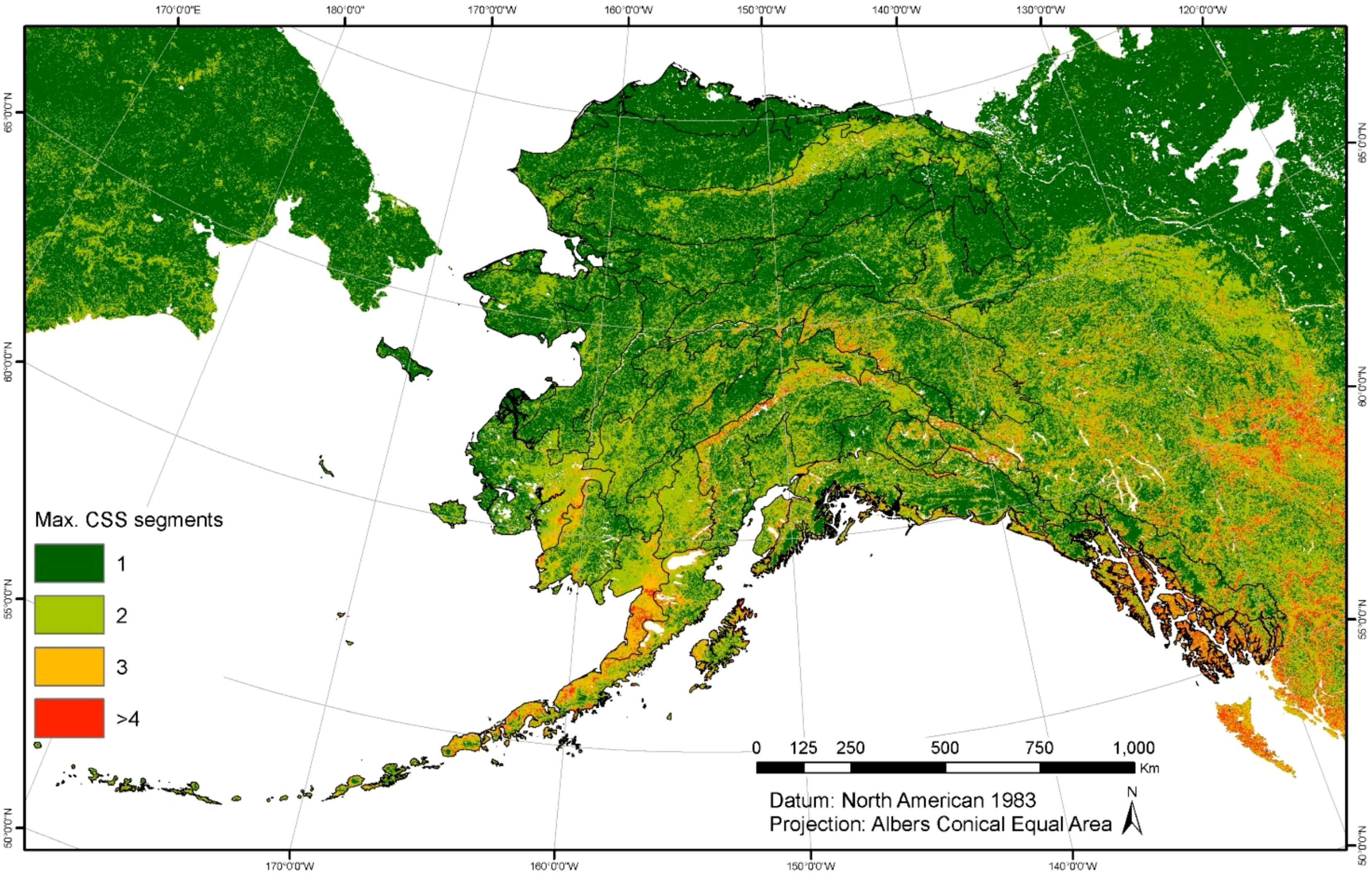
3.3.2. Continuous Snow Season

4. Conclusions
Supplementary Files
Supplementary File 1Acknowledgments
Author Contributions
Conflicts of Interest
References
- National Research Council. The Arctic in the Anthropocene: Emerging Research Questions; The National Academies Press: Washington, DC, USA, 2014; p. 4. [Google Scholar]
- Serreze, M.C.; Barry, R.G. Processes and impacts of Arctic amplification: A research synthesis. Glob. Planet. Change 2011, 77, 85–96. [Google Scholar] [CrossRef]
- Screen, J.A.; Simonds, I. The central role of diminishing sea ice in recent Arctic temperature amplification. Nature 2010, 464, 1334–1337. [Google Scholar] [CrossRef] [PubMed]
- Screen, J.A. The central role of diminishing sea ice in recent Arctic temperature amplification. Nat. Clim. Change 2014, 4, 577–582. [Google Scholar] [CrossRef]
- Lemke, P.; Ren, J.; Alley, R.; Allison, I.; Carrasco, J.; Flato, G.; Fujii, Y.; Kaser, G.; Mote, P.; Thomas, R.; Zhang, T. Chapter 4: Observations: Changes in snow, ice and frozen ground. In Climate Change 2007: The Physical Science Basis. Contribution of Working Group 1 to the Fourth Assessment Report of the Intergovernmental Panel on Climate Change; Solomon, S., Qin, D., Manning, M., Chen, Z., Marquis, M.C., Averyt, K., Tignor, M., Miller, H.L., Eds.; Intergovernmental Panel on Climate Change: Cambridge, UK and New York, NY, USA, 2007. [Google Scholar]
- Vihma, T. Effects of arctic sea ice decline on weather and climate: A review. Surv. Geophys. 2014, 35, 1175–1214. [Google Scholar] [CrossRef]
- Liston, G.E.; Hiemstra, C.A. The changing cryosphere: Pan-Arctic snow trends (1979–2009). J. Climate 2011, 24, 5691–5712. [Google Scholar] [CrossRef]
- PRISM Climate Group, Oregon State University. Available online: http://prism.oregonstate.edu (accessed on 20 February 2015).
- Scherrer, S.C.; Appenzeller, C.; Laternser, M. Trends in Swiss Alpine snow days: The role of local- and large-scale climate variability. Geophy. Res. Lett. 2004, 31. [Google Scholar] [CrossRef]
- Marty, C.; Meister, R. Long-term snow and weather observations at Wiessfluhjoch and its relation to other high-altitude observatories in the Alps. Theor. Appl. Climatol. 2012, 110, 573–583. [Google Scholar] [CrossRef]
- Peng, S.; Piao, S.; Ciais, P.; Friedlingstein, P.; Zhou, L.; Wang, T. Change in snow phenology and its potential feedback to temperature in the Northern Hemisphere over the last three decades. Environ. Res. Lett. 2013. [Google Scholar] [CrossRef]
- Garen, D.C.; Marks, D. Spatially distributed energy balance snowmelt modelling in a mountainous river basin: Estimation of meteorological inputs and verification of model results. J. Hydrol. 2005, 315, 126–153. [Google Scholar] [CrossRef]
- Xu, X.; Li, J.; Tolson, B. Progress in integrating remote sensing data and hydrologic modeling. Prog. Phys. Geogr. 2014, 38, 464–498. [Google Scholar] [CrossRef]
- Gao, Y.; Xie, H.; Yao, T.; Xue, C. Integrated assessment on multi-temporal and multi-sensor combinations for reducing cloud obscuration of MODIS snow cover products of the Pacific Northwest USA. Remote Sens. Environ. 2010, 114, 1662–1675. [Google Scholar] [CrossRef]
- Hall, D.K.; Solomonson, V.V.; Riggs, G.A. MODIS/Terra Snow Cover Daily L3 Global 500 m Grid. Version 5. NASA National Snow and Ice Data Center Distributed Active Archive Center: Boulder, CO, USA. Available online: http://dx.doi.org/10.5067/63NQASRDPDB0 (accessed on 4 September 2015).
- Hall, D.K.; Solomonson, V.V.; Riggs, G.A. MODIS/Aqua Snow Cover Daily L3 Global 500m Grid. Version 5. NASA National Snow and Ice Data Center Distributed Active Archive Center: Boulder, CO, USA. Available online: http://dx.doi.org/10.5067/ZFAEMQGSR4XD (accessed on 4 September 2015).
- Hall, D.K.; Riggs, G.A. Accuracy assessment of the MODIS snow products. Hydrol. Process. 2007, 21, 1534–1547. [Google Scholar] [CrossRef]
- Paintner, T.H.; Rittger, K.; McKenzie, C.; Slaughter, P.; Davis, R.E.; Dozier, J. Retrieval of subpixel snow covered area, grain size, and albedo from MODIS. Remote Sens. Environ. 2009, 113, 868–879. [Google Scholar] [CrossRef]
- Hall, D.K.; Riggs, G.A.; Salomonson, V.V.; DiGirolamo, N.E.; Bayr, K.J. MODIS snow-cover products. Remote Sens. Environ. 2002, 83, 181–194. [Google Scholar] [CrossRef]
- Parajka, J.; Blöschl, G. Spatio-temporal combination of MODIS images-potential for snow cover mapping. Water Resour. Res. 2008, 44, W030406. [Google Scholar] [CrossRef]
- Wang, X.; Xie, H.; Liang, T. Evaluation of MODIS snow cover and cloud mask and its application in Northern Xinjiang, China. Remote Sens. Environ. 2008, 112, 1497–1513. [Google Scholar] [CrossRef]
- Dietz, A.J.; Wohner, C.; Kuenzer, C. European snow cover characteristics between 2000 and 2011 derived from improved MODIS daily snow cover products. Remote Sens. 2012, 4, 2432–2454. [Google Scholar] [CrossRef]
- Paudel, K.P.; Andersen, P. Monitoring snow cover variability in an agropastoral area in the Trans Himalayan Region of Nepal using MODIS data with improved cloud removal methodology. Remote Sens. Environ. 2011, 115, 1234–1246. [Google Scholar] [CrossRef]
- Gafurov, A.; Bárdossy, A. Cloud removal methodology from MODIS snow cover product. Hydrol. Earth Syst. Sci. 2009, 13, 1361–1373. [Google Scholar] [CrossRef]
- Liang, T.G.; Huang, X.D.; Wu, C.X.; Liu, X.Y.; Li, W.L.; Guo, Z.G.; Ren, J.Z. An application of MODIS data to snow cover monitoring in a pastoral area: A case study in northern Xinjiang, China. Remote Sens. Environ. 2008, 112, 1514–1526. [Google Scholar] [CrossRef]
- Homer, C.C.; Huang, L.; Yang, B.; Wylie, B.; Coan, M. Development of a 2001 national landcover database for the United States. Photogramm. Eng. Remote Sens. 2004, 70, 829–840. [Google Scholar] [CrossRef]
- National Land Cover Database. Available online: http://www.mrlc.gov/ (accessed on 21 April 2015).
- Climate of Alaska. Available online: http://www.wrcc.dri.edu/narratives/alaska/ (accessed on 20 February 2015).
- L’Heureux, M.L.; Mann, M.E.; Gleason, B.E.; Vose, R.S. Atmospheric circulation influences on seasonal precipitation patterns in Alaska during the latter 20th century. J. Geophys. Res. 2004, 109, D06106. [Google Scholar] [CrossRef]
- Simpson, J.J.; Hufford, G.L.; Fleming, M.D.; Berg, J.S.; Ashton, J. Long-term climate patterns in Alaskan surface temperature and precipitation and their biological consequences. IEEE Trans. Geosc. Remote Sens. 2002, 40, 1164–1184. [Google Scholar] [CrossRef]
- Sturm, M.; Holmgren, J.; Liston, G.E. A seasonal snow cover classification system for local to global applications. J. Climate 1995, 8, 1261–1283. [Google Scholar] [CrossRef]
- Liston, G.E.; Sturm, M. Global seasonal snow classification system [53°N, 122°W; 73°N, 173°E]. National Snow and Ice Data Center: Boulder, CO, USA, 2006. [Google Scholar]
- Nowacki, G.; Spencer, P.; Fleming, M.; Brock, T.; Joregnson, T. Ecoregions of Alaska: 2001; U.S. Geological Survey Open-File Report 02-297; Alaska Geographic Data Committee: Anchorage, AK, USA, 2001.
- King, M.D.; Platnick, S.; Menzel, W.P.; Ackerman, S.A.; Hubanks, P.A. Spatial and temporal distribution of clouds observed by MODIS onboard the Terra and Aqua satellites. IEEE Trans. on Geosc. Remote Sens. 2013, 51, 3826–3852. [Google Scholar] [CrossRef]
- Frei, A.; Tedesco, M.; Lee, S.; Foster, J.; Hall, D.K.; Kelly, R.; Robinson, D.A. A review of global satellite-derived snow products. Adv. Space Res. 2012, 50, 1007–1029. [Google Scholar] [CrossRef]
- Parajka, J.; Holko, L.; Kostka, Z.; Blöschl, G. MODIS snow cover mapping accuracy in a small mountain catchment—Comparison between open and forest sites. Hydrol. Earth Syst. Sci. 2012, 16, 2365–2377. [Google Scholar] [CrossRef]
- Choi, G.; Robinson, D.A.; Kang, S. Changing northern hemisphere snow seasons. J. Climate 2010, 23, 5305–5310. [Google Scholar] [CrossRef]
- Brown, R.D.; Brasnett, B.; Robinson, D. Gridded North American monthly snow depth and snow water equivalent for GCM evaluation. Atmos.-Ocean 2003, 41, 1–14. [Google Scholar] [CrossRef]
- Alaska Snow Survey Program. Available online: http://www.nrcs.usda.gov/wps/portal/nrcs/main/ak/snow/ (accessed on 14 February 2014).
- Alaska Climate Research Center. Available online: http://climate.gi.alaska.edu (accessed on 17 January 2014).
- xmACIS2. Available online: http://xmacis.rcc-acis.org/ (accessed on 18 February 2014).
- Global Historical Climatology Network-Daily. Available online: https://www.ncdc.noaa.gov/oa/climate/ghcn-daily/ (accessed on 18 February 2014).
- MODIS Snow Metrics. Available online: https://github.com/gina-alaska/modis-snow-metrics (accessed on 26 April 2015).
- EXELIS Visual Information Systems. Available online: http://exelisvis.com/ (accessed on 21 May 2015).
- Singh, P.; Singh, V.P. Snow and Glacier Hydrology; Kluwer Academic Publishers: Dordrecht, The Netherlands, 2001; p. 236. [Google Scholar]
- Riggs, G.A.; Hall, D.K.; Salomonson, V.V. MODIS snow products user guide collection 5. Available online: http://modis-snow-ice.gsfc.nasa.gov/uploads/sug_c5.pdf (accessed on 4 September 2015).
- Klein, A.G.; Barnett, A.C. Validation of daily MODIS snow cover maps of the upper Rio Grande River Basin for the 2000–2001 snow year. Remote Sens. Environ. 2003, 86, 162–176. [Google Scholar] [CrossRef]
- Li, D.; Durand, M.; Margulis, S.A. Potential for hydrologic characterization of deep mountain snowpack via passive microwave remote sensing in the Kern River basin, Sierra Nevada, USA. Remote Sens. Environ. 2012, 125, 34–48. [Google Scholar] [CrossRef]
- R Project for Statistical Computing. Available online: https://www.r-project.org/ (accessed on 4 September 2015).
- Hüsler, F.; Jonas, T.; Musial, J.P.; Wunderle, S. A satellite-based snow cover climatology (1985–2011) for the European Alps derived from AVHRR data. Cryosphere 2014, 8, 73–90. [Google Scholar] [CrossRef]
- Hall, D.K.; Foster, J.L.; Verbyla, D.L.; Klein, A.G.; Benson, C.S. Assessment of snow-cover mapping accuracy in a variety of vegetation-cover densities in central Alaska. Remote Sens. Environ. 1998, 66, 129–137. [Google Scholar] [CrossRef]
- Parajka, J.; Pepe, M.; Rampini, A.; Rossi, S.; Blöschl, G. A regional snow-line method for estimating snow cover from MODIS during cloud cover. J. Hydrol. 2010, 381, 203–212. [Google Scholar] [CrossRef]
- Macander, M.J.; Swingley, C.S.; Joly, K.; Raynolds, M.K. Landsat-based snow persistence map for northwest Alaska. Remote Sens. Environ. 2015, 163, 23–31. [Google Scholar] [CrossRef]
- MODIS Snow Metrics. Available online: http://snow.proto.gina.alaska.edu/metrics (accessed on 26 April 2015).
- MODIS Snow Metrics. Available online: http://dds.gina.alaska.edu/public/NPS_products/MODIS_snow/ (accessed on 26 April 2015).
© 2015 by the authors; licensee MDPI, Basel, Switzerland. This article is an open access article distributed under the terms and conditions of the Creative Commons Attribution license (http://creativecommons.org/licenses/by/4.0/).
Share and Cite
Lindsay, C.; Zhu, J.; Miller, A.E.; Kirchner, P.; Wilson, T.L. Deriving Snow Cover Metrics for Alaska from MODIS. Remote Sens. 2015, 7, 12961-12985. https://doi.org/10.3390/rs71012961
Lindsay C, Zhu J, Miller AE, Kirchner P, Wilson TL. Deriving Snow Cover Metrics for Alaska from MODIS. Remote Sensing. 2015; 7(10):12961-12985. https://doi.org/10.3390/rs71012961
Chicago/Turabian StyleLindsay, Chuck, Jiang Zhu, Amy E. Miller, Peter Kirchner, and Tammy L. Wilson. 2015. "Deriving Snow Cover Metrics for Alaska from MODIS" Remote Sensing 7, no. 10: 12961-12985. https://doi.org/10.3390/rs71012961