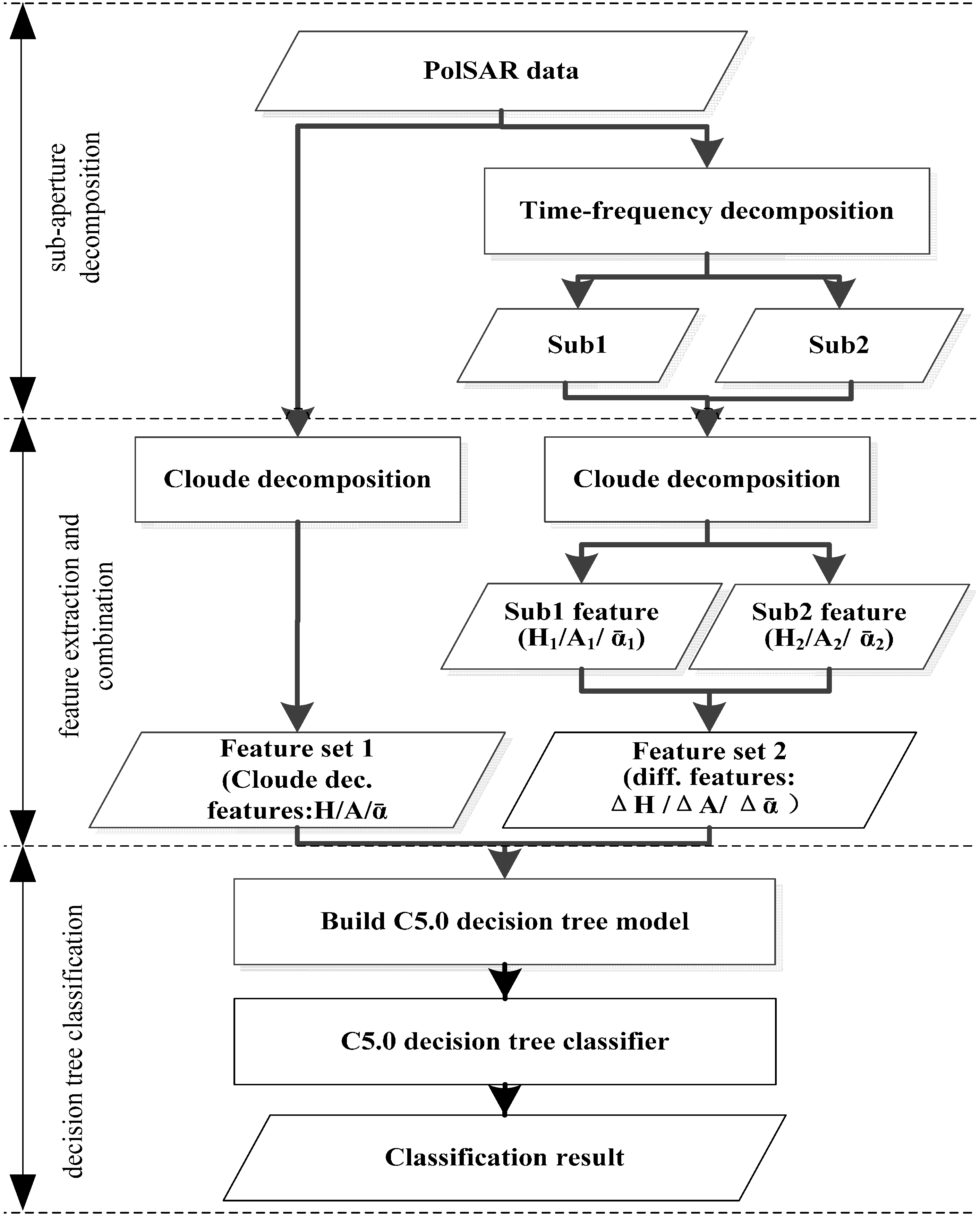
Article

Use of Sub-Aperture Decomposition for Supervised PolSAR Classification in Urban Area

College of Resource Environment and Tourism, Capital Normal University, Beijing 100048, China
*
Author to whom correspondence should be addressed.
Remote Sens. 2015, 7(2), 1380-1396; https://doi.org/10.3390/rs70201380
Submission received: 4 June 2014 / Accepted: 21 January 2015 / Published: 27 January 2015
(This article belongs to the Special Issue Remote Sensing Dedicated to Geographical Conditions Monitoring)

Abstract

:
A novel approach is proposed for classifying the polarimetric SAR (PolSAR) data by integrating polarimetric decomposition, sub-aperture decomposition and decision tree algorithm. It is composed of three key steps: sub-aperture decomposition, feature extraction and combination, and decision tree classification. Feature extraction and combination is the main contribution to the innovation of the proposed method. Firstly, the full-resolution PolSAR image and its two sub-aperture images are decomposed to obtain the scattering entropy, average scattering angle and anisotropy, respectively. Then, the difference information between the two sub-aperture images are extracted, and combined with the target decomposition features from full-resolution images to form the classification feature set. Finally, C5.0 decision tree algorithm is used to classify the PolSAR image. A comparison between the proposed method and commonly-used Wishart supervised classification was made to verify the improvement of the proposed method on the classification. The overall accuracy using the proposed method was 88.39%, much higher than that using the Wishart supervised classification, which exhibited an overall accuracy of 69.82%. The Kappa Coefficient was 0.83, whereas that using the Wishart supervised classification was 0.56. The results indicate that the proposed method performed better than Wishart supervised classification for landscape classification in urban area using PolSAR data. Further investigation was carried out on the contribution of difference information to PolSAR classification. It was found that the sub-aperture decomposition improved the classification accuracy of forest, buildings and grassland effectively in high-density urban area. Compared with support vector machine (SVM) and QUEST classifier, C5.0 decision tree classifier performs more efficient in time consumption, feature selection and construction of decision rule.

1. Introduction

Classification is one of the most important applications of Polarimetric synthetic aperture radar (PolSAR) images, especially in urban areas [1,2,3]. The rich information obtained from the backscatter signal of the ground features and polarimetric target decomposition of the echo signals [4] contains the electromagnetic scattering characteristics of the target objects, and it is usually used in understanding the scattering characteristics [4] and classification of the ground features [5,6,7,8,9,10]. Entropy/Alpha/Anisotropy–Wishart is one of the most famous PolSAR classification methods [11]. In this approach, the PolSAR data is first initialized by the Cloude–Pottier decomposition [9], and then the maximum likelihood classification is applied to extract the best-fit complex Wishart distribution [12] of the samples. But this method requires that the distribution of ground features follow a normal probability distribution function [13]. The complex distribution of ground features, especially for those in high-density urban area, often violates this premise and leads to poor classification results.
A full-resolution PolSAR image is obtained by synthesizing the signals scattered from the target in all azimuths [14]. The azimuth dependent backscattering is related to the type of target. The back-scattering of the same target under different azimuths would be different [15], as it is called anisotropy. But these differences have not been fully considered yet [14,15,16]. Sub-aperture decomposition technique [17], also known as time-frequency analysis, can make use of this different information from the changing azimuths. In recent years, progresses have been increasingly achieved by applying the sub-aperture decomposition to the target detection and extraction of the ground features. Ainsworth analyzed the high correlation between the sub-aperture images and extracted non-stationary targets from high-resolution PolSAR image [17]; Reigber detected the architectural structure in urban areas by verifying the point scatter with high correlation between the sub-apertures [18]; Runkle built the relationship between the irradiation direction and object orientation, and extracted the artificial targets through Hidden Markov Model (HMM) [19]. Good results can be obtained by using some of the above methods, but they require high intensity computation (e.g., coherence between the two sub-aperture) or complex algorithm (e.g., statistical inference on the distribution of surface features).
The purpose of the current study is to assess the potential of applying sub-aperture decomposition and Cloude–Pottier decomposition jointly to classify the PolSAR image. The core of the approach is the extraction and application of the feature set acquired by implementing Cloude–Pottier decompositions on the full-resolution PolSAR image and its sub-aperture images. Decision tree classifier [20] can be used for classification. It can efficiently select the most important features and give a better understanding of the results.

2. Experimental Data

The study area is located in San Francisco, CA, USA. The PolSAR data set used here is acquired by the C-band Airborne-Synthetic Aperture Radar (AIRSAR) in the NASA/JPL on 15 July 1994. The look angle ranges from 21.5° to 71.4°. The range resolution is about 6.6 m, and the azimuth resolution is about 9.3 m. In order to maintain the spatial resolution of the data, the original data without further processing (de-speckling) is used as the experimental data (Figure 1).
Figure 1. AIRSAR C-band polarimetric image of San Francisco with Pauli color-coding (Red: |HH − VV|, Green: |HV|, Blue: |HH + VV|). HH (horizontal transmit and horizontal receive), HV (horizontal transmit and vertical receive), VV (vertical transmit and vertical receive).
Remotesensing 07 01380 g001
It can be seen from the experimental data (Figure 1) that there are mainly four classes of ground covers, i.e., sea surface, vegetation, buildings and quasi-natural surface. The quasi-natural surface includes bare grounds, parking lots, sand, etc. The vegetation consists of forest and grassland. The building is divided into two parts based on the orientation of the building relative to the radar line of sight [21]. One is considered as the ortho-building (pink), which is vertical to the radar line-of-sight, and the other is considered as slant-building (green) whose main scatter center is at an oblique direction with the respect to the radar illumination. To simplify the process, 6 classes were selected to represent ground features in the study: water, forest, grassland, ortho-building, slant-building and others (quasi-natural surfaces).
The samples, which will be divided into the training and validation sets, were manually and randomly selected based on the optical image applied by Google Earth. The optical image was used to distinguish the ground truth, which was acquired in August 1993 and has a resolution about 1 m high precision in the buildings area. The number of samples for each class was determined according to the proportion of the class and the balance between the other classes. In order to show clearly, the distribution of the samples is shown on span image in Figure 2. Table 1 presents the number of pixels selected for the training and validation sets of each class.
Figure 2. The distribution of the samples shown on the span image.
Remotesensing 07 01380 g002
Table 1. Statistical chart of the sample data.
ClassTraining (Pixels)Validation (Pixels)Total
Water6656654013,196
Forest8508841734
Grassland103110902121
Ortho-Building137313122685
Slant-Building156316423205
Others152214893011
Total12,99512,95725,952

3. Methodology

The main procedure consists of three parts (Figure 3): sub-aperture decomposition, feature extraction and combination, and decision tree classification. The steps are detailed below:
Figure 3. Flow chart of the PolSAR image classification combining with the sub-aperture decomposition.
Remotesensing 07 01380 g003

3.1. Sub-Aperture Decomposition

Every pixel in SAR image does not correspond to a single observation of sight, but to a certain range of azimuthal look angle. This series of azimuthal look angle is defined as sub-aperture, and sub-aperture images can be obtained by performing the sub-aperture decomposition [15,16] on the full-resolution PolSAR image under certain azimuthal look angle. The transient characteristics of the target under different azimuthal look angles in the scattering of the electromagnetic waves are different. Therefore, the polarimetric information and physical characteristics of the targets could be mined by using the difference information of the echo waves scattered from the targets in the sub-aperture images. Moreover, the classification characteristics representing different scattering types are extracted and used in ground feature classification. In this section, two sub-aperture images under different azimuthal look angles are generated.

3.2. Feature Extraction and Combination

Cloude–Pottier decomposition is applied to the PolSAR images to obtain the feature set 1: scattering entropy (H), anisotropy (A) and scattering angle ( α ¯ ) The Cloude–Pottier decomposition is also conducted on the two sub-aperture images, respectively, and feature set 2, with its elements of ΔH, ΔA and Δ α ¯ is obtained through the differences between H, A and α ¯ of each sub-aperture image, respectively. Feature set 1 and 2 are combined to form the feature set for the target identification. The technology is introduced in detail as follows.
Cloude–Pottier decomposition [22] is an eigenvector analysis method based on coherence matrix. The polarimetric coherence matrix [T] is decomposed into the sum of three independent coherence matrices [Tn]:
[ T ] = i = 1 3 λ i [ T i ] = λ 1 e 1 e 1 * + λ 2 e 2 e 2 * + λ 3 e 3 e 3 *
where i represents the scattering mechanism; [ T i ] denotes an independent coherence matrix with rank 1 under a certain scattering mechanism; λ i denotes the eigenvalue, which represents the intensity of the scattering mechanism; e i is the eigenvector, which can be written as:
e i = e i i [ cos α i sin α i cos β i e i δ i sin α i sin β i e i γ i ] T
where α i corresponds to the physical mechanism of the process of target scattering, and its range is 0°~90°; β i denotes the azimuth angle of the target relative to the radar line-of-sight; i , δ i , and γ i are phase angles of target scattering [22]. In order to better describe the stochastic characteristics of media, Cloude and Pottier [10,23] gave the definitions as follows:
P i = λ i j = 1 3 λ j
H = i = 1 3 P i log 3 P i
α ¯ = i = 1 3 P i α i
A = λ 2 λ 3 λ 2 + λ 3
where P i is the probability obtained from the eigenvalue of [T]. H is the scattering entropy (0 ≤ H ≤ 1), and represents the stochastic characteristic of the target from isotropic scattering (H = 0) to complete stochastic scattering (H = 1). α ¯ is the scattering angle, representing the change of average scattering mechanisms from odd scattering ( α ¯ = 0°) to dipole scattering ( α ¯ = 45°) and then to even scattering ( α ¯ = 90°) [23]. The anisotropy A characterizes the relative magnitudes of the second and third eigenvalues. A 5 × 5 window was chosen when calculating H/alpha decomposition.
As a result of Cloude–Pottier decomposition to the full-resolution PolSAR image, entropy (H), anisotropy (A) and alpha ( α ¯ ) are taken as feature set 1. Besides, the differences information (ΔH, ΔA and Δ α ¯ ) between the results of the Cloude–Pottier decomposition to the two sub-aperture images are taken as feature set 2, which is defined as follows:
Δ H = H 2 H 1
Δ A = A 2 A 1
Δ α ¯ = α ¯ 1 α ¯ 2
where H i , A i and α ¯ ( i = 1 ,   2 ) represent polarimetric entropy, anisotropy and average scattering angle of the two sub-apertures. Feature set 2 are combined with feature set 1 to identify ground targets.
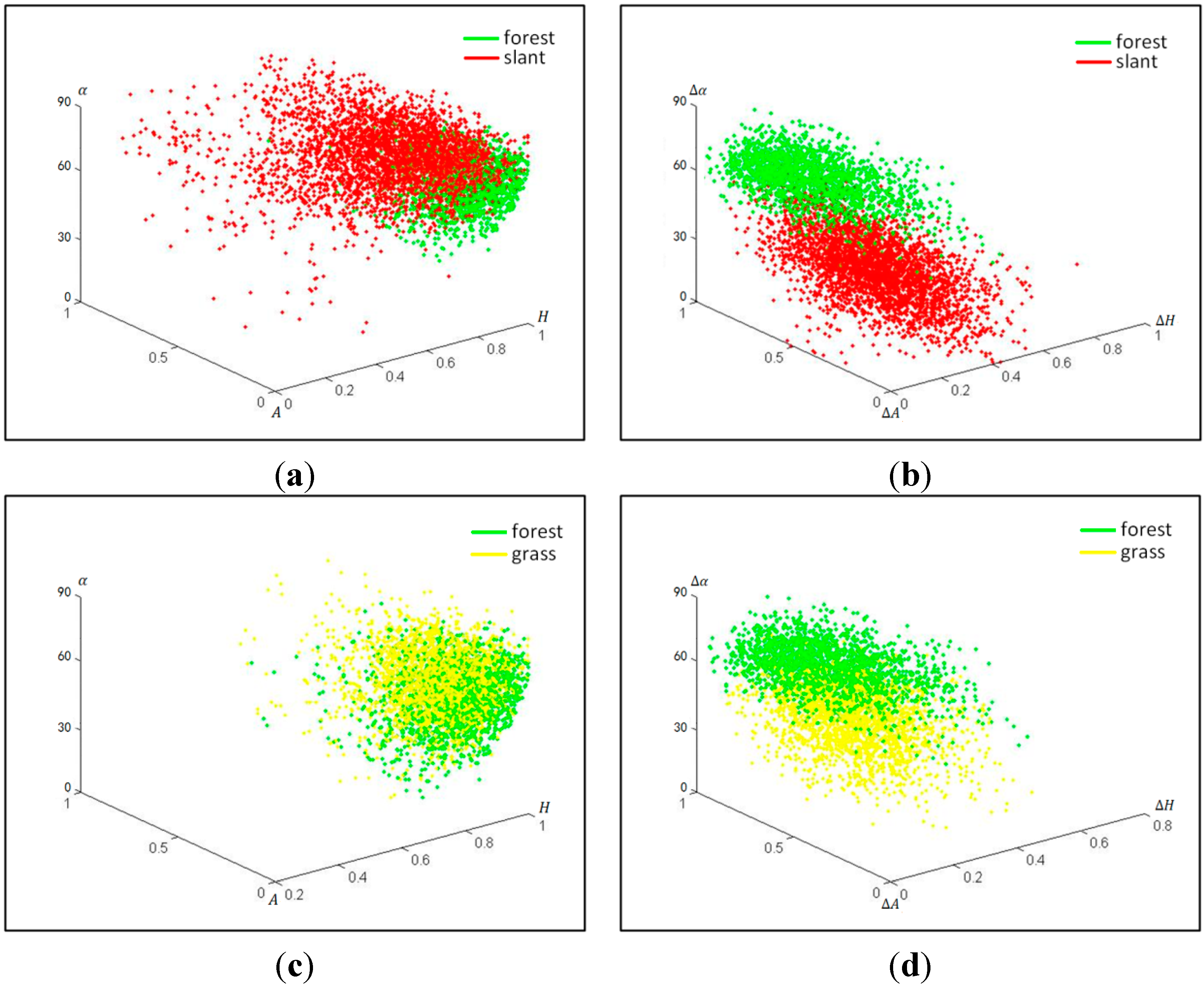
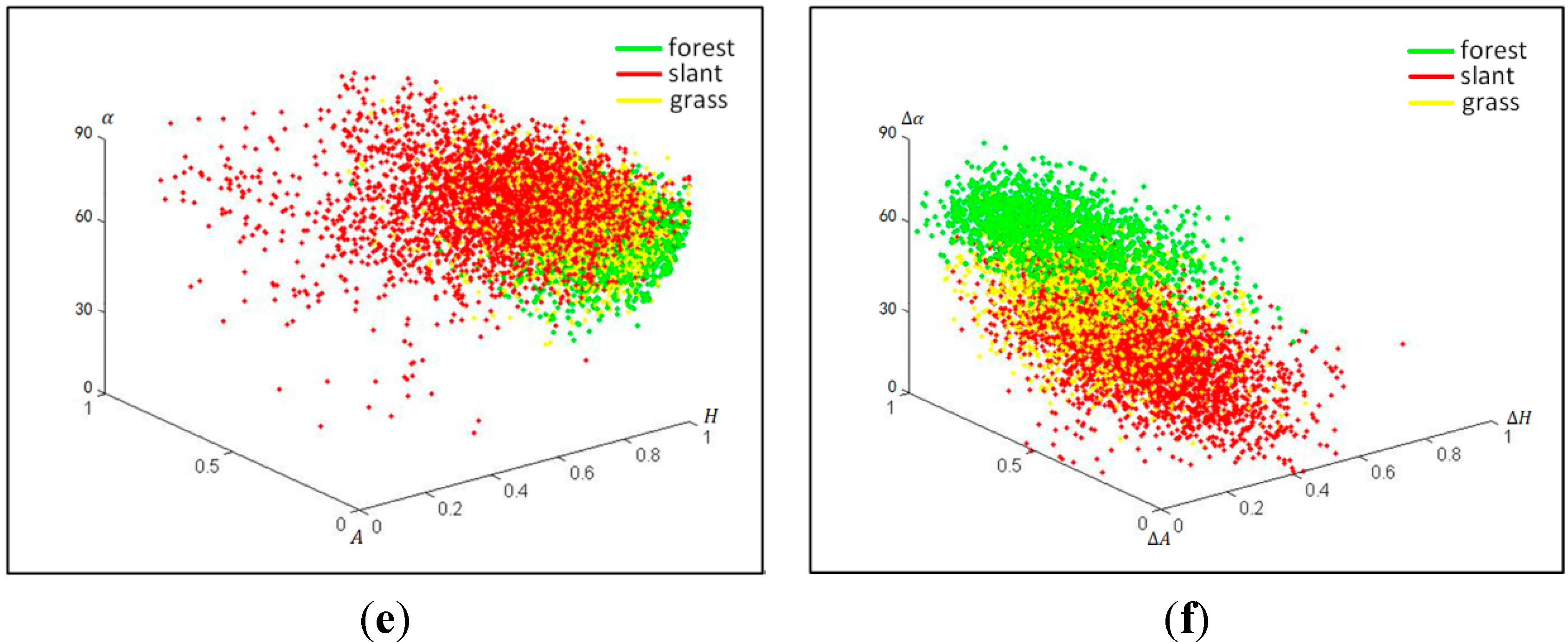
To further understand the capability of distinguishing ground features using feature set 1 and 2, the training samples of forest, grassland and slant-buildings were selected, and their scatter diagrams were plotted using feature set 1 and 2, respectively (Figure 4). Red points are the slant-buildings, green points are forest and yellow points are grassland.
As shown in Figure 4, feature set 2 can distinguish slant-buildings from forest (Figure 4b), and it can improve the separability between forest and grassland (Figure 4d). In Figure 4f, grassland and slant-buildings are mixed slightly but it performs better than feature set 1 (Figure 4e). In summary, feature set 2, compared with feature set 1, can mine more information from the original PolSAR image, and is more suitable for ground feature identification.
Figure 4. The scatter diagrams of forest, slant-buildings and grassland in feature set 1 and 2. Scattering entropy (H), anisotropy (A) and scattering angle ( α ¯ ) are decomposed from the PolSAR image. The same Cloude–Pottier decomposition is also conducted on the two sub-aperture images, respectively, and feature set 2, with its elements ΔH, ΔA and α ¯ , is obtained through the differences between H, A and α ¯ of each sub-aperture image, respectively. (a) Feature set 1: forest and slant-buildings; (b) Feature set 2: forest and slant-buildings; (c) Feature set 1: forest and grassland; (d) Feature set 2: forest and grassland; (e) Feature set 1: forest, grassland and slant-buildings; (f) Feature set 2: forest, grassland and slant-buildings.
Remotesensing 07 01380 g004aRemotesensing 07 01380 g004b

3.3. Decision Tree Classification

Different from the Maximum Likelihood classification method based on the statistical distribution function, the decision tree is a classifier with high speed, high accuracy, simple generation mode and applicability to large datasets [24]. Not requiring pre-decided data distribution, this algorithm is popularly used in data mining for complicated, non-linear mapping. Here we used C5.0 [25] decision tree to construct the classification rules because it has the following features: (1) generation of intuitive rules, enhancing user understanding of the algorithm; (2) robustness to missing data; (3) fast operation speed; (4) a powerful boosting technique, i.e., boosting and cost-sensitive tree building [26].
In this study, feature set 1 and the 2 were combined into a multichannel image. A feature vector was then formed for each of the selected 25,952 pixels (Table 1). Twelve thousand nine hundred and ninety-five training pixels (vectors) were used to develop the C5.0 decision tree model, and then the classification result is applied to the 12,957 validation pixels using the developed C5.0 tree to evaluate the classification accuracy.

4. Results and Discussion

4.1. Comparison between the Proposed Method and the Wishart Supervised Classification

The results of the proposed method are compared to that of the Wishart supervised classification method [13] to verify the improvement of the proposed method on the classification. Our research is mainly about the application of the new method in urban area (as marked with red rectangle in Figure 1), thus comparisons of the classification results in urban area are shown in Figure 5.
Figure 5. Classification Results of Wishart supervised and proposed method. (a) Classification result obtained by Wishart supervised classification method; and (b) Classification result obtained by the proposed method.
Remotesensing 07 01380 g005
From Figure 5, it can be seen that the classification result obtained by Wishart supervised classification method (Figure 5a) are generally greenish. Most of the slant-buildings are classified as forest improperly. However, the proposed method (Figure 5b) shows a good discriminate ability of the ground features. The buildings and vegetation are well distinguished.
To verify the improvement that the proposed method brings to the classification accuracy, quantitative analysis was made through four parameters, namely, overall accuracy (OA), Kappa Coefficient, user’s accuracy (UA) and producer’s accuracy (PA) [27]. The confusion matrices of classification results are shown as follows (Table 2 and Table 3).
Table 2. Confusion matrix of Wishart supervised classification method. (PA = producer’s accuracy, UA =user’s accuracy, OA =overall accuracy).
ClassWaterForestGrasslandOrtho-BuildingSlant-BuildingOthersPA (%)
Water6257131680010295.67
Forest583564220321640.27
Grassland4430659541103154.59
Ortho-Building049222499535738.03
Slant-Building35188647916592240.13
Others599341680768145.74
UA (%)89.4837.6326.7884.0149.0779.28
OA (%): 69.82 Kappa Coefficient: 0.56
Table 3. Confusion matrix of the proposed classification method. (PA = producer’s accuracy, UA =user’s accuracy, OA =overall accuracy).
ClassWaterForestGrasslandOrtho-BuildingSlant-BuildingOthersPA (%)
Water6433714008698.36
Forest187091210112580.20
Grassland131386311519010357.89
Ortho-Building00711461491087.35
Slant-Building0191807112868678.32
Others851855677124883.81
UA (%)98.2379.5762.6092.5775.0780.10
OA (%): 88.39 Kappa Coefficient: 0.83
From Table 2 and Table 3, it can be readily seen that the overall accuracy using the proposed method is 88.39%, much higher than that using the Wishart supervised classification, which exhibits an overall accuracy of 69.82%. The Kappa Coefficient is 0.83, whereas that using the Wishart supervised classification is 0.56. Through the confusion matrix (Table 2), it can be seen that there are a lot of misclassifications among slant-buildings, forest and grassland. However, the misclassifications have been decreased obviously using the proposed methods. The UA values of grassland and forest using Wishart supervised classification method are only 26.78% and 37.63%, while those using proposed method are increased by 35.82% and 41.94%, respectively. Taking the slant-buildings as an example, the UA of slant-buildings using the Wishart supervised classification method is 49.07%. However, in the proposed method, it is increased by 26.00%.
The application of Wishart supervised classification method requires the ground features statistical distribution conforms to a certain probability distribution function. When the distribution of the ground features is complex or PolSAR data with the high spatial resolution are used, this assumption is always hard to be satisfied. For example, the experimental area is a high-density urban area, so the Wishart classifier’s assumption is not applicable. However, decision tree model does not require such assumptions, and it is more suitable for supervised classification of PolSAR data in complex ground features [28]. The sub-aperture decomposition is not used at this point. Fortunately it improves the classification accuracy from the perspective of multiple features.

4.2. Influence of Sub-Aperture Decomposition

In this section, the H/A/ α ¯ -C5 method was designed to find out the contribution of sub-aperture decomposition used in the proposed method. In the proposed method, both feature set 1 (H, A and α ¯ from the full-resolution PolSAR image) and feature set 2 (difference information between the two sub-aperture images) were input into the C5.0 decision tree algorithm, while only feature set 1 were used for H/A/ α ¯ -C5 method. In this way, the influence of the sub-aperture decomposition brought to the proposed method could be dug out. In order to take a closer view of the classification results, a subset is used to show the differences between using H/A/ α ¯ -C5 and the proposed method (Figure 6).
Figure 6. Details of the Classification Results from H (entropy)/A (anisotropy)/ α ¯ (scattering angle)-C5 and proposed method. (a) ground truth; (b) H/A/ α ¯ -C5; (c) proposed method.
Remotesensing 07 01380 g006
From Figure 6, as the results of classification using H/A/ α ¯ -C5, it can be seen that most of the grassland has been mistakenly classified as others, and the forest in the middle of the picture were misclassified as slant-buildings. However, the proposed method can effectively avoid the misclassifications referred to above, as well as obtain a better visual consequent of the six ground features.
The importance of every feature was calculated in SPSS Clementine v14.2, and sorted in descending order. The importance of H, Δ α ¯ , α ¯ -A, ΔA and ΔH is 0.23, 0.21, 0.17, 0.16, 0.13, 0.10, respectively. The features extracted from sub-aperture decomposition are as important as Cloude–Pottier decomposition. Δ α ¯ plays an essential role in the proposed method. Due to all the features that work together in the classification process, the quality of image classification has improved significantly.
The confusion matrix of the H/A/ α ¯ -C5 method (Table 4) was calculated with the experimental data and the detailed quantitative analysis are given by comparison with the proposed method (Table 3).
Table 4. Confusion Matrix of H (entropy)/A (anisotropy)/ α ¯ (scattering angle)-C5 Classification Method. (PA = producer’s accuracy, UA =user’s accuracy, OA =overall accuracy).
ClassWaterForestGrasslandOrtho-BuildingSlant-BuildingOthersPA (%)
Water6429115009598.3
Forest155991740435367.76
Grassland2525447082587543.12
Ortho-Building0041143162387.12
Slant-Building4511748512903878.56
Others1463889997111074.55
UA (%)97.1362.8551.3191.8169.7380.79
OA (%): 85.21 Kappa Coefficient: 0.79
It was illustrated by the result of comparing with Table 3 and Table 4 that the sub-aperture decomposition played a limited role, as the OA and Kappa Coefficient of the proposed method are only increased by 0.0318 and 0.04, respectively. However, when a more detailed comparison was performed on the PA and UA of these two methods, the advantages of the sub-aperture decomposition became more apparent. It can be seen from Table 3 and Table 4, that the misclassifications of forest and grassland are the most serious. A certain proportion of the grassland is mistakenly classified as forest and slant-buildings. The values of PA and UA are 43.12% and 51.31%, respectively. The polarization orientation angle shifts are induced by surfaces with nonzero azimuth slopes as well as by man-made targets that are not aligned in the along-track direction [29]. These shifts produce higher cross-polarization (HV) intensity and make coherency or covariance matrix reflection asymmetrical. The ratio of the cross-polarized component, which mainly contributes to the volume scattering power, increases in the slant-buildings whose main scatter center is at an oblique direction with the respect to the radar illumination. However, using the proposed method, classification accuracies of forest, grassland and slant-buildings are obviously improved. The result of quantitative analysis is consistent with that of the visual interpretation. The PA and UA of grassland are increased by 14.77% and 11.29%, and those of forest are increased by 12.44% and 16.72%. Additionally, the UA of the slant-building is increased by 5.34% as the reduction of misclassifications of forest and grassland. The misclassifications of forest in the H/A/ α ¯ -C5 method are 43 samples, whereas that of in the proposed method is only 11 samples.
The difference between the proposed method and the H/A/ α ¯ -C5 method is whether or not the sub-aperture decomposition features are input into the C5.0 decision tree algorithm, therefore, a conclusion can be drawn that the improvement of classification accuracy of the objects including forest, grassland and slant-buildings is due to the injection of sub-aperture decomposition. When the full decomposition-based classification method (e.g., Wishart and H/A/ α ¯ -C5 method) is used on C-band PolSAR data, the forest and grassland cannot be distinguished. By imaging the same target from different angles, the slight differences between the forest and the grassland can be found in the Sub-aperture images in C-band. As a result, sub-aperture decomposition can distinguish the forest and the grassland so effectively that it can be used to improve the accuracy of classification.

4.3. Comparison among Different Classifiers

In order to investigate the contribution of C5.0 classifier to the final accuracy, two typical classifiers are used to classify the study area with the same feature set as the proposed method, which include Support Vector Machine (SVM) [30] and Quest [28]. Comparisons of the classification results are shown in Figure 7.
Figure 7. Details of the Classification Results. (a) Ground truth; (b) Support Vector Machine (SVM); (c) Quest; (d) proposed method.
Remotesensing 07 01380 g007
The image of the ground truth is applied by Google Earth (Figure 7a). It is used to distinguish the ground truth. From the perspective of the classification of slant-building, using SVM and Quest classifier can lead to an over-classification. Roads will be classified as slant-buildings, while using C5.0 decision tree roads and slant-buildings can be better distinguished. It can be inferred from the classification of grassland that it still has a poor performance, though the result of using C5.0 decision tree algorithm is superior to the other two classifiers.
The confusion matrixes of the classification methods, using SVM and Quest (Table 5 and Table 6), were calculated and the detailed quantitative analysis are given by comparison with the proposed method (Table 3).
Table 5. Confusion Matrix of Classification Method using Support Vector Machine (SVM). (PA = producer’s accuracy, UA =user’s accuracy, OA =overall accuracy).
ClassWaterForestGrasslandOrtho-BuildingSlant-BuildingOthersPA (%)
Water63508560083797.09
Forest11462463008370.59
Grassland17084509320711746.70
Ortho-Building30511631132888.64
Slant-Building42313564125913976.67
Others971361536841661941.57
UA (%)93.7166.9555.0389.662.8660.51
OA (%): 81.22 Kappa Coefficient: 0.73
Table 6. Confusion Matrix of Classification Method using Quest. (PA = producer’s accuracy, UA =user’s accuracy, OA =overall accuracy).
ClassWaterForestGrasslandOrtho-BuildingSlant-BuildingOthersPA (%)
Water62747800018895.93
Forest346961121281378.76
Grassland6015649762908145.60
Ortho-Building01571125165785.75
Slant-Building5132588130121079.23
Others52736381212575150.44
UA (%)90.9370.0273.2091.3168.1560.41
OA (%): 82.03 Kappa Coefficient: 0.74
The selection of the classifier has a great influence on classification results. The OA and Kappa Coefficient of the classification using C5.0 decision tree are increased by about 6% and 0.1 compared with the classifications using QUEST decision tree and SVM.
The influence of classifier on the accuracy of slant-buildings, others and grassland is obvious. Others refer to quasi-natural surfaces. Although the PA values of the three methods are similar, the application of SVM classifier to slant-buildings classification made an over-classification. The UA values of slant-building using SVM and Quest classifier are 62.86% and 68.15%, while that using the proposed method is 75.07%. The PA values of others using C5.0 decision tree, QUEST decision tree and SVM are 83.81%, 50.44% and 41.57%, respectively. The UA value of others using C5.0 decision tree increased by 20% compared with those using the other classifiers. The PA value of grassland using C5.0 decision tree increased by 12% compared with those using QUEST decision tree and SVM, while The UA value of grassland using C5.0 decision tree decreased by 10.6% compared with that using QUEST decision tree. The application of C5.0 classifier to grassland classification made an over-classification.
C5.0 decision tree has a better performance on feature space optimization and feature selection, especially when the feature set is large [20,24]. SVM is computationally expensive, as it is required to be trained and evaluated a large number of times with different subsets of features in order to achieve a group of optimization parameters [30]. The decision tree can provide clear classification rules that can be easily interpreted based on the physical meaning of the features. The rule of C5.0 tree is more complex than QUEST but it allows for more than the two subgroups of segmentation many times. QUEST decision tree is designed to reduce the processing time required for the large decision tree analysis [31]. In the condition of a small feature set, the complex rules built by C5.0 decision tree are more conducive to accurate classification.

5. Conclusions

In this paper, an approach for classifying the PolSAR data by integrating polarimetric decomposition, sub-aperture decomposition and decision tree algorithm is proposed. The sub-aperture decomposition showed great capability on distinguishing between slant-buildings and vegetation (forest and grassland) on C-band PolSAR data. As a result, the proposed method improved the PolSAR data classification dramatically. Its performance was compared with that of Wishart supervised classification.
The proposed method has the following advantages: (1) it has high practicality because the PolSAR data is not strictly required. Although many studies have shown that multi-band classification technology, such as multi-frequency and PolSAR interferometry, can improve the classification accuracy. In practical applications, it is often difficult to meet the data requirements of these methods. The proposed method is more convenient because high classification accuracy could be achieved by only one PolSAR data band. (2) It is simple and fast. Polarimetric decomposition, sub-aperture decomposition and C5.0 decision tree algorithm, as the three components of the proposed method, are well developed and easy to use, so that both complicated pre-processing (e.g., registration in multi-band classification method) and intensive computation (e.g., polarimetric interferometry) can be avoided. (3) It is a white box. The given classifier or classification rule reveals the ground types associated with specific features. Therefore, unlike black box algorithms (such as neural network, etc.), the proposed method can give a clear physical explanation. (4) No assumptions on the distribution of ground features are demanded. In conclusion, this approach provides a superior way of classifying PolSAR data.
Although the producer’s accuracy of grassland has been improved by using the proposed method, it still has a poor performance because of azimuth slopes affect the relative magnitude and phase of the polarimetric coherence matrix and similitude of scattering characteristics between lawn and others. To resolve this disadvantage, a further research will be done.

Acknowledgments

This research is supported by Beijing Natural Science Foundation, Project No.: 4142011, and National Natural Science Foundation of China, Project No.: 40801172. The authors would like to thank JPL AIRSAR for providing valuable polarimetric SAR.

Author Contributions

Lei Deng conducted the study and developed the proposed methodology. Lei Deng was responsible for data pre-processing. Ya-nan and Yan Chen Sun carried out the results validation and analysis. Chen Sun wrote the manuscript. Lei Deng and Ya-nan Yan were involved in discussing its results and correcting the manuscript.

Conflicts of Interest

The authors declare no conflict of interest.

References

  1. Yu, J.; Yan, Q.; Zhang, Z.; Ke, H.; Zhao, Z.; Wang, W. Unsupervised classification of polarimetric synthetic aperture radar images using kernel fuzzy c-means clustering. Int. J. Image Data Fusion 2012, 3, 319–332. [Google Scholar] [CrossRef]
  2. Brook, A.; Ben-Dor, E.; Richter, R. Modelling and monitoring urban built environment via multi-source integrated and fused remote sensing data. Int. J. Image Data Fusion 2013, 4, 2–32. [Google Scholar] [CrossRef]
  3. Dickinson, C.; Siqueira, P.; Clewley, D.; Richard, L. Classification of forest composition using polarimetric decomposition in multiple landscapes. Remote Sens. Environ. 2013, 131, 206–214. [Google Scholar] [CrossRef]
  4. Boerner, W.M.; Yan, W.-L.; Xi, A.Q.; Yamaguchi, Y. On the basic principles of radar polarimetry: The target characteristic polarization state theory of kennaugh, huynen’s polarization fork concept, and its extension to the partially polarized case. IEEE Proc. 1991, 79, 1538–1550. [Google Scholar] [CrossRef]
  5. Del Frate, F.; Latini, D.; Pratola, C.; Palazzo, F. Pcnn for automatic segmentation and information extraction from x-band sar imagery. Int. J. Image Data Fusion 2013, 4, 75–88. [Google Scholar]
  6. Vanzyl, J.J. Unsupervised classification of scattering behavior using radar polarimetry data. IEEE Trans. Geosci. Remote Sens. 1989, 27, 36–45. [Google Scholar] [CrossRef]
  7. Park, S.E.; Moon, W.M. Unsupervised classification of scattering mechanisms in polarimetric sar data using fuzzy logic in entropy and alpha plane. IEEE Trans. Geosci. Remote Sens. 2007, 45, 2652–2664. [Google Scholar] [CrossRef]
  8. Kourgli, A.; Ouarzeddine, M.; Oukil, Y.; Belhadj-Aissa, A. Texture modelling for land cover classification of fully polarimetric sar images. Int. J. Image Data Fusion 2012, 3, 129–148. [Google Scholar] [CrossRef]
  9. Cloude, S.R.; Pottier, E. A review of target decomposition theorems in radar polarimetry. IEEE Trans. Geosci. Remote Sens. 1996, 34, 498–518. [Google Scholar] [CrossRef]
  10. Trisasongko, B.H. The use of polarimetric SAR data for forest disturbance monitoring. Sens. Imaging: Int. J. 2010, 11, 1–13. [Google Scholar] [CrossRef]
  11. Potier, E.; Lee, J.S. Unsupervised classification scheme of polSAR images based on the complex Wishart distribution and the “H/A/alpha” polarimetric decomposition theorem. In Proceedings of the EUSAR 2000, Munich, Germany, 23–25 May 2000; pp. 265–268.
  12. Conradsen, K.; Nielsen, A.A.; Sehou, J.; Skriver, H. A test statistic in the complex wishart distribution and its application to change detection in polarimetric sar data. IEEE Trans. Geosci. Remote Sens. 2003, 41, 4–19. [Google Scholar] [CrossRef]
  13. Lee, J.S.; Grunes, M.R. Classification of multi-look polarimetric SAR data based on complex Wishart distribution. In Proceedings of the 1992 IEEE National Telesystems Conference, George Washington University, Virginia Campus, Washington, DC, USA, 19–20 May 1992; pp. 21–24.
  14. Ainsworth, T.L.; Lee, J.S. Polarimetric SAR image classification employing subaperture polarimetric analysis. In Proceedings of the 2005 IEEE International Geoscience and Remote Sensing Symposium, Seoul, Korea, 25–29 July 2005; pp. 41–43.
  15. Ainsworth, T.L.; Jansen, R.W.; Lee, J.S.; Fiedler, R. Sub-aperture analysis of high-resolution polarimetric SAR data. In Proceedings of the 1999 IEEE International Geoscience and Remote Sensing Symposium, Hamburg, Germany, 28 June–2 July 1999; pp. 41–43.
  16. Ferro-Famil, L.; Reigber, A.; Pottier, E.; Boerner, W.M. Analysis of anisotropic behavior using sub-aperture polarimetric SAR data. In Proceedings of the 2003 IEEE International Geoscience and Remote Sensing Symposium, Toulouse, France, 21–25 July 2003; pp. 434–436.
  17. Ferro-Famil, L.; Reigber, A.; Pottier, E. Nonstationary natural media analysis from polarimetric sar data using a two-dimensional time-frequency decomposition approach. Can. J. Remote Sens. 2005, 31, 21–29. [Google Scholar]
  18. Reigber, A.; Jager, M.; He, W.; Ferro-Famil, L.; Hellwich, O. Detection and classification of urban structures based on high-resolution SAR imagery. In Proceedings of the 2005 IEEE International Urban Remote Sensing Joint Event, Paris, France, 11–13 April 2007; pp. 1–6.
  19. Runkle, P.; Nguyen, L.H.; McClellan, J.H.; Carin, L. Multi-aspect target detection for sar imagery using hidden markov models. IEEE Trans. Geosci. Remote Sens. 2001, 39, 46–55. [Google Scholar]
  20. Chen, M. Comparing traditional statistics, decision tree classification and support vector machine techniques for financial bankruptcy prediction. Intell. Autom. Soft Comput. 2012, 18, 65–73. [Google Scholar]
  21. Kimura, H. Radar polarization orientation shifts in built-up areas. IEEE Trans. Geosci. Remote Sens. 2008, 5, 217–221. [Google Scholar]
  22. Cloude, S.R. Target decomposition theorems in radar scattering. Electron. Lett. 1985, 21, 22–24. [Google Scholar] [CrossRef]
  23. Cloude, S.R.; Pottier, E. An entropy based classification scheme for land applications of polarimetric sar. IEEE Trans. Geosci. Remote Sens. 1997, 35, 68–78. [Google Scholar]
  24. Wang, Y.Y.; Li, J. Feature-selection ability of the decision-tree algorithm and the impact of feature-selection/extraction on decision-tree results based on hyperspectral data. Int. J. Remote Sens. 2008, 29, 2993–3010. [Google Scholar]
  25. Pang, S.L.; Gong, J.Z. C5.0 classification algorithm and application on individual credit evaluation of banks. Syst. Eng.—Theory Pract. 2009, 29, 94–104. [Google Scholar]
  26. Freund, Y.; Schapire, R.E. A decision-theoretic generalization of on-line learning and an application to boosting. J. Comput. Syst. Sci. 1997, 55, 119–139. [Google Scholar] [CrossRef]
  27. Story, M.; Congalton, R.G. Accuracy assessment-a user’s perspective. Photogramm. Eng. Remote Sens. 1986, 52, 397–399. [Google Scholar]
  28. Qia, Z.; Yeh, A.G.O.; Li, X.; Zheng, L. A novel algorithm for land use and land cover classification using RADARSAT-2 polarimetric SAR data. Remote Sens. Environ. 2012, 118, 21–39. [Google Scholar] [CrossRef]
  29. Lee, J.S.; Ainsworth, T.L. The effect of orientation angle compensation on coherency matrix and polarimetric target decompositions. IEEE Trans. Geosci. Remote Sens. 2011, 49, 53–64. [Google Scholar]
  30. Lardeux, C.; Frison, P.L.; Rudant, J.P.; Souyris, J.C. Use of the SVM classification with polarimetric SAR data for land use cartography. In Proceedings of the 2006 IEEE International Geoscience and Remote Sensing Symposium, Denver, CO, USA, 31 July–4 August 2006; pp. 493–496.
  31. Lim, T.S.; Loh, W.Y.; Shih, Y.S. A comparison of prediction accuracy, complexity, and training time of thirty-three old and new classification algorithms. Machine Learning 2000, 40, 203–228. [Google Scholar] [CrossRef]

