Article

Meeting Earth Observation Requirements for Global Agricultural Monitoring: An Evaluation of the Revisit Capabilities of Current and Planned Moderate Resolution Optical Earth Observing Missions

by
Alyssa K. Whitcraft
1,*,
Inbal Becker-Reshef
1,†,
Brian D. Killough
2,† and
Christopher O. Justice
1
1
Department of Geographical Sciences, University of Maryland, College Park, 4321 Hartwick Rd. Suite 410, College Park, MD 20742, USA
2
National Aeronautics and Space Administration—Langley Research Center, Committee on Earth Observation Satellites Systems Engineering Office, Hampton, VA 23681, USA
*
Author to whom correspondence should be addressed.
These authors contributed equally to this work.
Remote Sens. 2015, 7(2), 1482-1503; https://doi.org/10.3390/rs70201482
Submission received: 30 September 2014 / Accepted: 14 January 2015 / Published: 29 January 2015
(This article belongs to the Special Issue Remote Sensing in Food Production and Food Security)

Abstract

:
Agriculture is a highly dynamic process in space and time, with many applications requiring data with both a relatively high temporal resolution (at least every 8 days) and fine-to-moderate (FTM < 100 m) spatial resolution. The relatively infrequent revisit of FTM optical satellite observatories coupled with the impacts of cloud occultation have translated into a barrier for the derivation of agricultural information at the regional-to-global scale. Drawing upon the Group on Earth Observations Global Agricultural Monitoring (GEOGLAM) Initiative’s general satellite Earth observation (EO) requirements for monitoring of major production areas, Whitcraft et al. (this issue) have described where, when, and how frequently satellite data acquisitions are required throughout the agricultural growing season at 0.05°, globally. The majority of areas and times of year require multiple revisits to probabilistically yield a view at least 70%, 80%, 90%, or 95% clear within eight days, something that no present single FTM optical observatory is capable of delivering. As such, there is a great potential to meet these moderate spatial resolution optical data requirements through a multi-space agency/multi-mission constellation approach. This research models the combined revisit capabilities of seven hypothetical constellations made from five satellite sensors—Landsat 7 Enhanced Thematic Mapper (Landsat 7 ETM+), Landsat 8 Operational Land Imager and Thermal Infrared Sensor (Landsat 8 OLI/TIRS), Resourcesat-2 Advanced Wide Field Sensor (Resourcesat-2 AWiFS), Sentinel-2A Multi-Spectral Instrument (MSI), and Sentinel-2B MSI—and compares these capabilities with the revisit frequency requirements for a reasonably cloud-free clear view within eight days throughout the agricultural growing season. Supplementing Landsat 7 and 8 with missions from different space agencies leads to an improved capacity to meet requirements, with Resourcesat-2 providing the largest incremental improvement in requirements met. The best performing constellation can meet 71%–91% of the requirements for a view at least 70% clear, and 45%–68% of requirements for a view at least 95% clear, varying by month. Still, gaps exist in persistently cloudy regions/periods, highlighting the need for data coordination and for consideration of active EO for agricultural monitoring. This research highlights opportunities, but not actual acquisition rates or data availability/access; systematic acquisitions over actively cropped agricultural areas as well as a policy which guarantees continuous access to high quality, interoperable data are essential in the effort to meet EO requirements for agricultural monitoring.

Graphical Abstract

1. Introduction

Remote sensing during the past decade has undergone what has been described as the “MODIS Revolution”, with nearly twice daily, consistently high quality global observations available in near real time (NRT) being used to generate global scale science results [1,2,3]. With the Landsat archive opening and computational resources growing, global scale analyses are poised to move into the moderate resolution domain [4,5,6,7,8], with regional to global datasets at 30 m resolution already demonstrated [9,10,11,12,13]. In the context of crop condition monitoring and yield forecasting, moderate resolution data have not yet achieved broad scale results across the globe, primarily due to the lack of consistent cloud free acquisitions with sufficiently high temporal resolution. However, as demonstrated by the Group on Earth Observations Global Agricultural Monitoring (GEOGLAM) initiative’s table of Earth observation (EO) data requirements (Table 1, especially Requirements #4–6; full discussion in Whitcraft et al. (this issue) [1]), this is a priority growth area for analyses spanning the extent of cropland for fields of all sizes.
Requirements for coarse resolution data are presently being met by the systematic acquisitions of systems like MODIS and its follow-on, the Visible Infrared Imaging Radiometer (VIIRS) Suite [14], as well as Proba-V and Sentinel-3. However, in terms of moderate spatial resolution optical missions, no single observatory at present is capable of acquiring data with sufficient frequency to meet an eight day reasonably cloud free requirement over all croplands [1], much less one which makes data freely and openly available. Still, the Landsat observatory has been used in many regional studies, particularly for land cover and land use analyses [11,15,16,17,18,19]. In the private sector, there are emerging options for both fine and moderate spatial resolution monitoring, such as Planet Labs and Disaster Modeling Constellation [20]. However, they are (or will be) fee-based, and are not yet established as a viable data source with sufficient calibration and testing. For this reason, the focus herein will be on analyzing the capability of current and near-term moderate resolution civil space agency flown instruments to meet EO requirements for global agricultural monitoring in the context of GEOGLAM.
The GEOGLAM community of practice [21], composed of agricultural monitoring experts from operational monitoring, research centers, and universities across the globe [22,23,24,25,26,27,28], together with the Committee on Earth Observation Satellites (CEOS) Ad Hoc Team for GEOGLAM [29] have developed a table documenting the EO data requirements for satellite-based monitoring of large-scale agriculture (Table 1). Based on this requirements table (specifically, Table 1, Requirement #5’s preferred temporal resolution of eight days), Whitcraft et al. (this issue) [1] have articulated spatially explicit (0.05°) temporal revisit requirements for reasonably cloud free moderate resolution optical monitoring (spanning the visible, reflected infrared, and thermal infrared portions of the electromagnetic spectrum) over within-season global agricultural areas. While the table requests “cloud free” data (Table 1, Column D), in fact reasonably cloud free data may suffice. As such, four definitions of reasonably cloud free were analyzed—70%, 80%, 90%, and 95%—with the required revisit frequency commonly falling in the two- to four-day range (depending on month and clarity thresholds).
From this, there remains the assessment of the capacity of our current and planned moderate resolution missions to meet these revisit frequency requirements for reasonably cloud free data within eight days during the agricultural growing season. This is achieved by identifying candidate missions and modeling their coincident orbital overpasses to form hypothetical multi-mission/multi-space agency constellations, then comparing their combined revisit capabilities with the required revisit frequencies established in Whitcraft et al. (this issue) [1]. While all four cloud free thresholds are analyzed, the 70% and 95% are specifically highlighted as bounding the upper (“best”) and lower (“worst”) cases, respectively. This reveals how and where we can (and cannot) meet moderate spatial resolution optical EO requirements for monitoring. In those areas where we cannot meet these requirements, alternative data types (namely, microwave synthetic aperture radar (SAR) data) should be considered. In fact, one of the GEOGLAM data requirements (Table 1, Requirement #6) calls for SAR data on an approximately weekly basis in areas that are “persistently cloudy,” in addition to rice cultivating areas. The term “persistently cloudy” is qualitative but carries the implication that areas which fit this description are those for which current/planned moderate resolution optical instrumentation are insufficient. Therefore, “persistently cloudy” will be defined herein as those areas and times of year which require a more frequent revisit in order to yield a reasonably clear view than our current/planned moderate resolution optical missions are capable of delivering.
Table 1. The table of requirements for satellite-based Earth observations data, developed by the Committee on Earth Observation Satellites (CEOS) Ad Hoc Team for Group on Earth Observations Global Agricultural Monitoring (GEOGLAM) [21,29]. Requirements are broken down by spatial and spectral range (Columns B and C), frequency with which reasonably cloud free data are required (Column D), geographic extent (Columns E and F), as well as the application or target product for which the data would be used (Columns G–M). Requirements are further refined based on the field size over which acquisitions are required (Column F), or the field sizes for which a certain data type would be useful (Columns G–M). “L” refers to “Large fields” (defined as >15 ha), “M” refers to “Medium fields” (defined as 1.5–15 ha), and “S” refers to “small fields” (<1.5 ha). The symbol “x” or the word “All” indicate that these data are useful for that product generation for all field sizes.
ABCDEFGHIJKL M
Spatial ResolutionSpectral RangeEffective observ. frequency (cloud free)ExtentField SizeTarget Products
Req#Crop MaskCrop Type Area and Growing CalendarCrop Condition IndicatorsCrop YieldCrop Biophys. VariablesEnviron. VariablesAg Practices/Cropping Systems
Coarse Resolution Sampling (>100 m)
1500–2000 mopticalDailyWall-to-WallAll X L
2100–500 moptical2 to 5 per weekCropland extentAllXXXLLXL
35–50 kmmicrowaveDailyCropland extentAll XXXX
Moderate Resolution Sampling (10 to 100 m)
410–70 mopticalMonthly (min 3 in season + 2 out of season); Required every 1–3 yearsCropland extent (if #5 = sample, else skip)AllXL/M X
510–70 moptical8 days; 1 min per 16 daysSample (pref. Cropland extent)AllXXXXXXX
610–100 mSAR8 days; 1 min per 16 daysCropland extent of persistantly cloudy and rice areasAllXXXXXXX
Fine Resolution Sampling (5 to 10 m)
75–10 mVIS NIR + SWIRMonthly (3 min in season)Cropland extentM/SM/SM/S
85–10 mVIS NIR + SWIRApprox. weekly; 5 min per seasonSampleAll M/SX XXX
95–10 mSARMonthlyCropland extent of persistantly cloudy and rice areasM/SM/SM/S M/S
Very Fine Resolution Sampling (<5 m)
10<5 mVIS NIR3 per year (2 in season + 1 out of season); Every 3 yearsCropland extent of small fieldsSSS
11<5 mVIS NIR1 to 2 per monthRefined Sample (Demo)All X X X

Identifying Candidate Missions

There are a number of moderate resolution optical missions that are currently operating as well as several additional planned to launch in the next few years. As of late 2014, the only moderate resolution optical missions with free and open data policies are Landsat 7 Enhanced Thematic Mapper (L7 ETM+; [30]) and the Landsat 8 Operational Land Imager and Thermal Infrared Sensor (L8 OLI and TIRS; ibid), which together have a combined revisit capability of eight days (SLC-Off problems notwithstanding). However, due to onboard storage and downlinking limitations, these missions have not historically acquired every land scene at every opportunity. Notably, however, recent alterations to the missions’ acquisition plans have greatly increased daily acquisitions to 550–600 daylit scenes per day for L8 and 400–450 for L7 [31] from the originally partitioned 250 best quality daylit, land-containing scenes, coming close to acquiring all possible 540–630 daylit land-containing scenes within view of each sensor each day [32,33,34]. The Indian Space Research Organization’s (ISRO) Resourcesat-2 Advanced Wide Field Sensor (R2 AWiFS; [35]) is also currently operating, with a spatial resolution as fine as 55 m and a repeat cycle of 24 days, although with its sensor engineering characteristics, this permits a revisit capability on the order of five days. At present, ISRO does not provide this data freely to all and their nominal acquisition plan does not include coverage of global agricultural areas. Agencies within the United States—namely, the Department of Agriculture—have procured these data and found them to be valuable for cropland monitoring applications and compatible if not complementary to Landsat data, although some uncertainty about long term radiometric calibration stability remains [6,11,36]. Meanwhile, planned for the near future is the European Space Agency’s Sentinel-2 Earth observatory, made up of two separate satellites, each with the Multi-Spectral Instrument (MSI) on-board (S2A, S2B; [37]), the first of which is set for launch in 2015. The two satellites together are planned to systematically acquire all data over land in the low-latitudes every five days and in the mid-latitudes on the order of two to three days [38]. The Sentinel-2 program also plans to employ a free and open data policy, and efforts are underway to cross-calibrate the instruments and ensure interoperability with Landsat [8,39]. It should be noted that the Sentinel-2 MSI sensors do not include thermal bands. Thermal data in the agricultural monitoring context are used primarily for evapotranspiration and water status [40,41], and land surface temperature measurements [42,43], as well as for atmospheric adjustment [3,8,44], although there is recent research suggesting their utility in yield forecasting [45] as well as for crop type classification and residue mapping. Nevertheless, data from the visible, near-IR, and shortwave IR are still the most broadly applied resource in the agricultural monitoring context. Therefore, due to the Sentinel-2 missions’ MSI’s high spatial and temporal resolution, their free and open data policy, their planned interoperability with the Landsat missions, and their otherwise well-placed spectral bands, they are included herein for analysis. While there are other moderate resolution Earth observing missions in orbit or planned for launch within the next five years, these five instruments have (or will have) the highest quality data, are being studied for interoperability, and are considered to be the most attainable and highest quality by the CEOS Ad Hoc Team for GEOGLAM. They therefore comprise the candidate missions analyzed herein for their combined revisit capabilities.

2. Methods

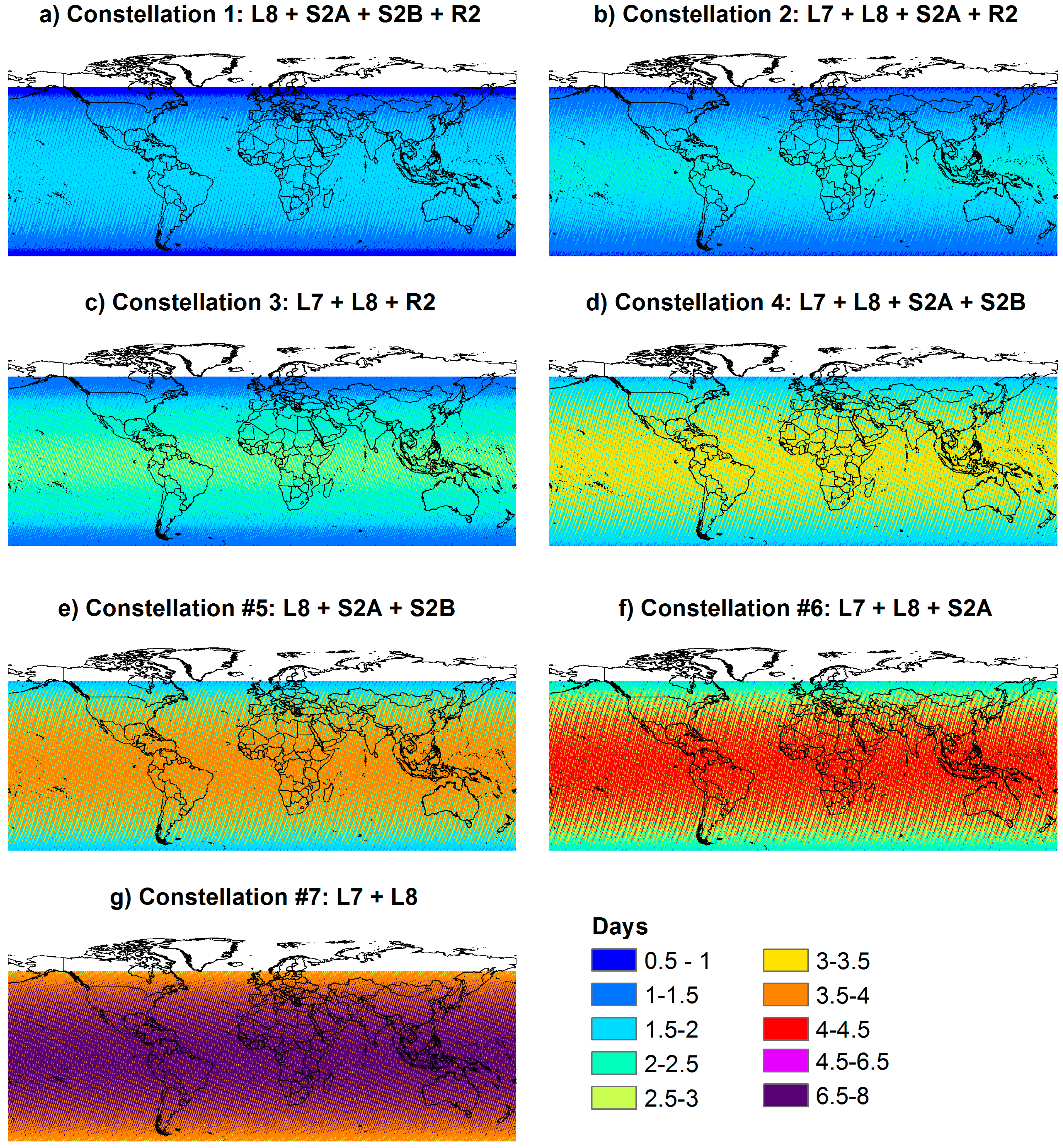
2.1. Overpass Analysis

The frequency with which a given area falls within the view of a satellite sensor is contingent upon the satellite’s orbit, the field of view of the sensor, and the latitude of the target area. With polar orbiters, high latitudes are within view more frequently than Equatorial zones, and so the variability in combined revisit capabilities occurs on a latitudinal gradient. Different missions have different repeat cycles, which refers to the time it takes the satellite to repeat a full orbital cycle (to be distinguished from revisit capabilities, which is the amount of time until an area is within view of a sensor). As such, it is necessary to evaluate the combined revisit capabilities of multiple sensors in a window of time (“scenario period”) sufficient to allow for all considered missions to complete their respective full repeat cycles on the same day, at least once (note that in the case of Constellation #7 in Table 2, the scenario period could have been 16 days; however, for computational simplicity in the simulation process, the period analyzed was lengthened to 80 days—5 completed scenarios–but this has no impact on the revisit frequency results). CEOS has invested in the development of the CEOS Visualization Environment (COVE) tool that models the orbits, and by extension, the coincident overpasses of multiple missions [46,47]. In this analysis, the aforementioned five satellites have been combined to form seven hypothetical imaging moderate resolution optical constellations (Table 2) run within the COVE system.
Table 2. The seven hypothetical constellations and the lengths of their scenario period.
Constellation #Satellites IncludedScenario Period—Days
1L8, S2A, S2B, R2160
2L7, L8, S2A, R2120
3L7, L8, R272
4L7, L8, S2A, S2B80
5L8, S2A, S2B 80
6L7, L8, S2A80
7L7, L8 80
Each time a given area passes within view of one sensor in a hypothetical constellation during its scenario period, it is counted as an acquisition opportunity (AO). In order to yield the average time to revisit for each 1° cell, at the end of the scenario period the number of AOs for each hypothetical constellation is divided by the number of days within the scenario period (Figure 1). For example, if Constellation #1 were to have 200 AOs in its 160 day scenario, the average time to revisit would be 0.8 days. The actual interval between AOs is variable throughout the scenario period and will be shorter or longer than the average as the scenario period progresses. However, this interval of AOs is not consistently bound to any point in time or any specific longitude (it is contingent upon the initial conditions of the simulation run in COVE); as such, the mode (most common) of these average revisit frequencies over each 1° increment of latitude has been extracted to be compared with the spatially explicit revisit frequencies required (from Whitcraft et al. (this issue) [1]) for the four reasonably cloud-free thresholds: 70%, 80%, 90%, and 95%.
This analysis shows coincident overpasses and therefore acquisition opportunities from 60° N to 60° S (where the majority of croplands lie), but does not attempt to analyze actual acquisition frequencies. As previously mentioned, of the observatories incorporated in this analysis, only the Sentinel-2 program (S2A/S2B) plans to acquire every (low- and mid-latitude) land scene at every opportunity, and therefore an acquisition opportunity does not automatically mean that an image will be acquired. This analysis provides a baseline of what kind of performance by these missions is possible.
Figure 1. The average revisit capabilities of the seven hypothetical constellations analyzed herein (ag). This is the “raw” revisit analysis, showing for each 1° cell the average revisit time observed over the scenario period. Because the variability across longitude is not significant, as it is tied to the initial conditions of the simulation, the most frequent (mode) revisit observed for each 1° of latitude has been extracted for use in this analysis.
Remotesensing 07 01482 g001

2.2. Comparing Overpass Capabilities with EO Requirements

Whitcraft et al. (this issue) [1], shows the revisit frequencies required (RFR) to yield a reasonably clear view (defined as having a final percentage clear (FPC) of at least 70%, 80%, 90%, or 95%) within 8 days over in-season (actively cropped, as defined by agricultural growing season calendars in Whitcraft et al. (2014) [48]) 0.05° agriculture-containing cells (as defined by the cropland mask in Fritz et al. (2015) [49]). For views at least 70% clear within 8 days, 44%–55% of in-season cropped cells worldwide (depending on the month) would require a revisit more frequent than 4 days, respectively. For views at least 95% clear, if data are required within 8 days, a revisit frequency of less than 4 days would be required in 76%–99% of actively cropped cells (depending on the month). Full dataset inputs, methods, results, and discussion regarding the derivation of these RFRs can be found in the accompanying manuscript. In this present manuscript, the focus is evaluating whether the mode (most common) revisit capabilities of each of the seven constellations introduced in the previous section (resampled to 0.05°) are frequent enough to meet the RFRs to yield a view at least 70%, 80%, 90%, or 95% clear within 8 days for each 0.05° cell. The FPC ≥ 70% case and the FPC ≥ 95% case are further highlighted as upper (“best case”) and lower (“worst case”) approximations, respectively, of our ability to meet this 8 day requirement for reasonably clear optical data.

3. Results

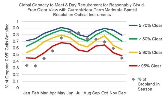
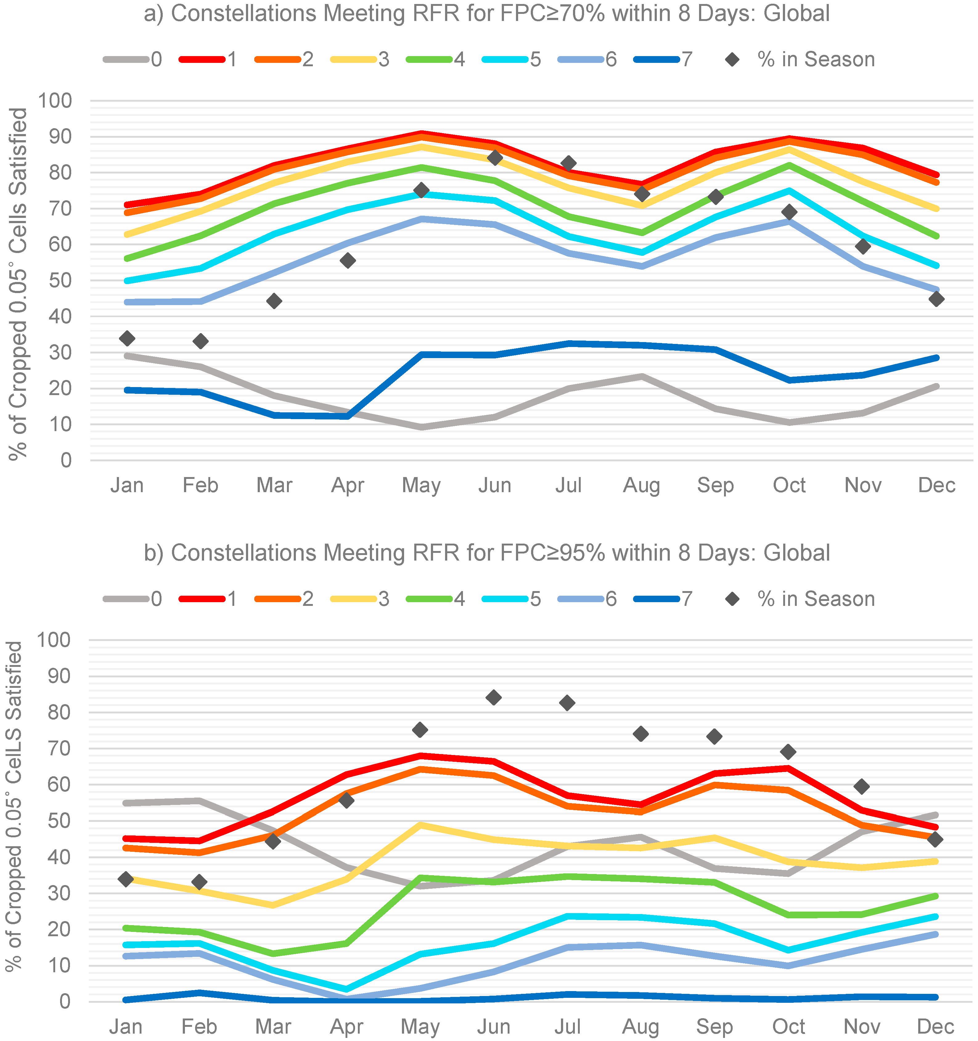
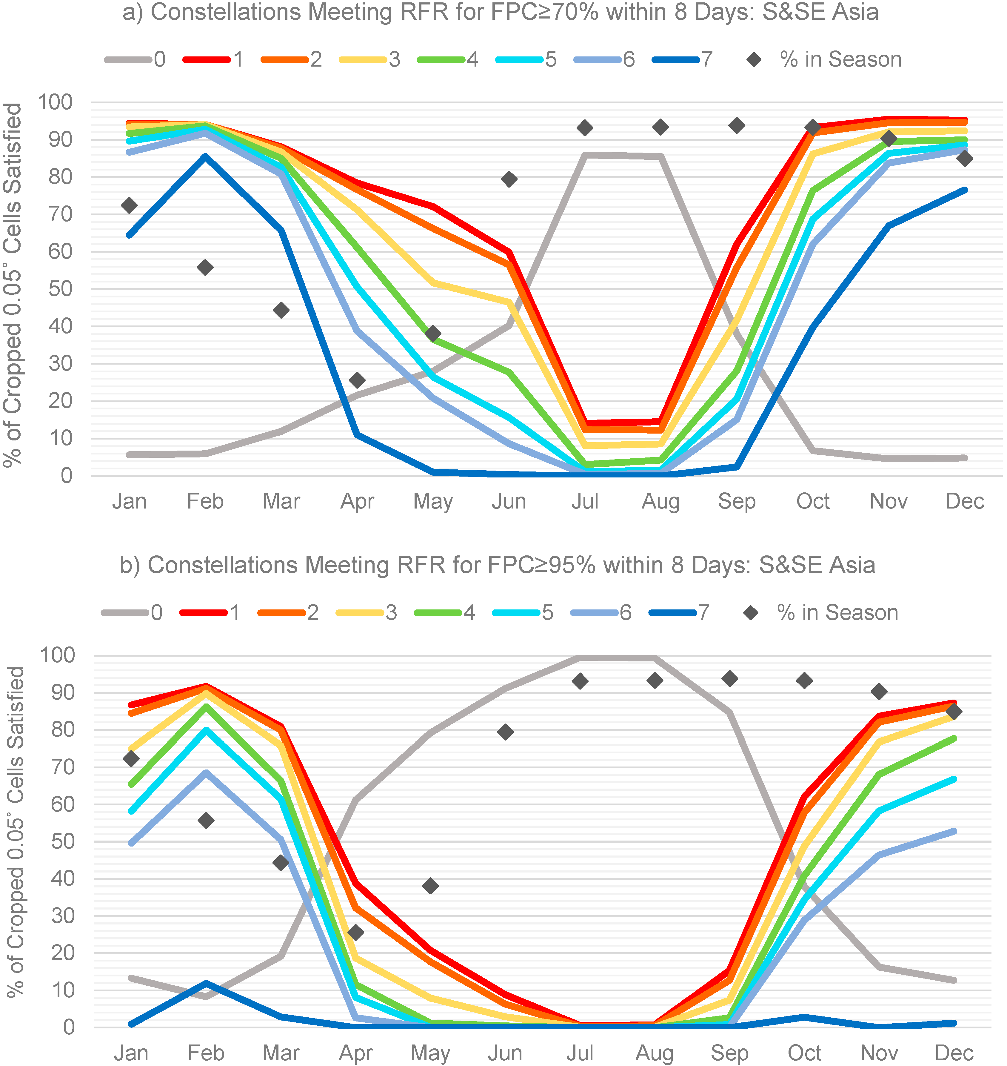
3.1. Meeting the Requirement for a Reasonably Clear View Every 8 Days

In Table 2, the constellations are numbered 1 through 7, which both identifies them and denotes their rank in terms of revisit frequency. That is to say, anything that Constellation #7 can meet, so too can #1–6, anything Constellation #6 can meet, so too can #1–5 but not #7, et cetera. Meanwhile, a value of 0 (denoted “None” in Figure 2) indicates that no constellation is capable of meeting the revisit frequency requirement (RFR), and denotes a time and area for which active microwave SAR data ought to be considered. The monthly maps showing which of the constellations are capable of meeting the less frequent required revisit for each month (based on a final percentage clear requirement of at least 70%; Figure 2) show that for most areas in most months, 6–7 different proposed constellations are capable of meeting the RFR for this best case scenario. The same, however, cannot be said for the worst case scenario (based on a final percentage clear requirement of at least 95%; Figure 2, right), wherein many areas are met by only Constellations #1–3, and still many others are not viable candidates for the use of optical data alone (shown in grey, and denoted as “None” or “0” in subsequent figures).
In fact, at the global level, Constellation #1 (most frequent revisit capability) can probabilistically meet an 8 day requirement for at least 70% cloud free data for between 71% (January) and 91% (May) of 0.05° cells worldwide (Figure 3). For at least 80% clear, 63%–87% of cells can have their requirements met; for at least 90% clear, 53%–80% can have their requirements met; and, for at least 95% clear, 45%–68% of cells can have their requirements met.
As of late 2014, Landsat 7 and Landsat 8 acquire the only freely and openly available moderate resolution data. Their combination, Constellation #7, even in the FPC ≥ 70% (“best case”) scenario (Figure 4a), can only meet an 8 day revisit requirement in 12%–32% of actively cropped 0.05˚ grid cells, and in virtually 0% of actively cropped cells for all months in the FPC ≥ 95% (“worst case”) scenario (Figure 4b).
Figure 2. Where which constellation is capable of meeting the revisit frequency required to yield a view of in-season croplands that is at least 70% ((left), “best case scenario”) or 95% ((right), “worst case scenario”) clear for the representative months of January, April, July, and October. In-season croplands have been defined by the growing season calendars from Whitcraft et al. (2014) [48] and the cropland mask from Fritz et al. (2015) [49]. The missions included in Constellations #1–7 can be found in Table 2. Note that constellation number both identifies the constellation, as well as denotes its rank in terms of revisit frequency (with #1 being capable of the most frequent revisit). Areas requiring a revisit more frequent that any hypothetical constellation analyzed herein are shown in gray, and denoted as “None.” Full map figures for all months can be found in Supplemental Materials.
Remotesensing 07 01482 g002
Figure 3. The overall capacity to meet an 8 day data requirement for data at least 70%, 80%, 90%, or 95% clear (FPC), as introduced in Whitcraft et al. (this issue) [1]. “Capacity” corresponds with the percentage of total actively cropped 0.05° cells which have their revisit frequency requirements satisfied by at least one constellation (i.e., the best/most frequent performer, Constellation #1). To provide perspective on the relative cropland area requiring imagery for each month, also plotted is the percentage of total global croplands which are in-season during each month, as indicated by Whitcraft et al. (2014) [48] and Fritz et al. (2015) [49].
Remotesensing 07 01482 g003
The addition of a single Sentinel-2 mission, as in Constellation #6, leads to a marked increase in the success rate in the best case scenario (44%–67%), although is less impactful in the worst case scenario (0–18%) (Figure 4). Meanwhile, the addition of R2 to the two Landsats (as in Constellation #3) increases the global success rate to 63%–87% (best case) and 27%–49% (worst case). Interestingly, Constellations #1–2’s inclusion of 4 instruments does not greatly improve upon Constellation #3 in the best case scenario, although in the worst case scenario, Constellation #2 does increase the success rate to 41%–64%. These examples highlight the importance of sensor architecture, as R2’s large swath width lends the largest improvement in success rate. Nevertheless, the addition of any single sensor to the current capabilities (Constellation #7) would improve revisit and therefore success rates, particularly when allowing for less stringent clarity thresholds.
These success rates, of course, vary greatly when taking a regional perspective, as cloud cover’s impact on obtaining (reasonably) clear views varies geographically and revisit capability varies latitudinally (more frequent revisits are possible at the poles than at the Equator). A region with a particularly strong seasonality is South/Southeast Asia, including India, Nepal, Burma, Bhutan, Bangladesh, Vietnam, Laos, Thailand, Cambodia, and Malaysia (Figure 5).
An analysis of this region shows a very large difference between the best (Figure 5a) and worst (Figure 5b) case scenarios during the middle of the year (April-September), although the general shapes of the curves are similar. This is due to the effects of the Indian Summer Monsoon, during which cloud obscuration is both pervasive and persistent [50]. As seen in Figure 5a, the success rate for the best case scenario for even Constellation #1 during July and August hovers around 15%, meaning approximately 85% of actively 0.05° cells are left without a view that is even 70% clear. Exacerbating this situation is the fact that July and August are among the most pervasively cropped months of the calendar year, meaning these requirements are unmet, not just at a higher rate but over a larger area. The outlook is even poorer in the worst case scenario (Figure 5b), where even Constellation #1’s success rate stays below 10% from June until September. However, from October through March, the cloud cover declines considerably and the success rates for multiple constellations are quite high. In this (and other) areas so seasonally impacted by cloud cover, SAR data alone and/or optical-SAR fused data should be further explored and implemented for agricultural monitoring [51,52,53].
Figure 4. Globally, the percent of actively cropped 0.05° cells in each month which have their requirement for (a) at least 70% clear views (“best case”); and (b) at least 95% clear views (“worst case”), every 8 days met by each constellation’s mode revisit rate (a value of “0” indicates no constellation is capable, and can be understood as the failure rate). To provide perspective on the relative cropland area requiring imagery for each month, also plotted is the percentage of total global croplands which are in-season during each month, as indicated by Whitcraft et al. (2014) [48] and Fritz et al. (2015) [49].
Remotesensing 07 01482 g004
Figure 5. For South and Southeast Asia (excluding China), the percent of actively cropped 0.05° cells in each month which have their requirement for (a) at least 70% clear views (“best case”); and (b) at least 95% clear views (“worst case”) every 8 days satisfied by each constellation’s mode revisit rate (a value of “0” indicates no constellation is capable, and can be understood as the failure rate). To provide perspective on the relative cropland area requiring imagery for each month, also plotted is the percentage of total croplands in this region which are in-season during each month, as indicated by Whitcraft et al. (2014) [48] and Fritz et al. (2015) [49].
Remotesensing 07 01482 g005

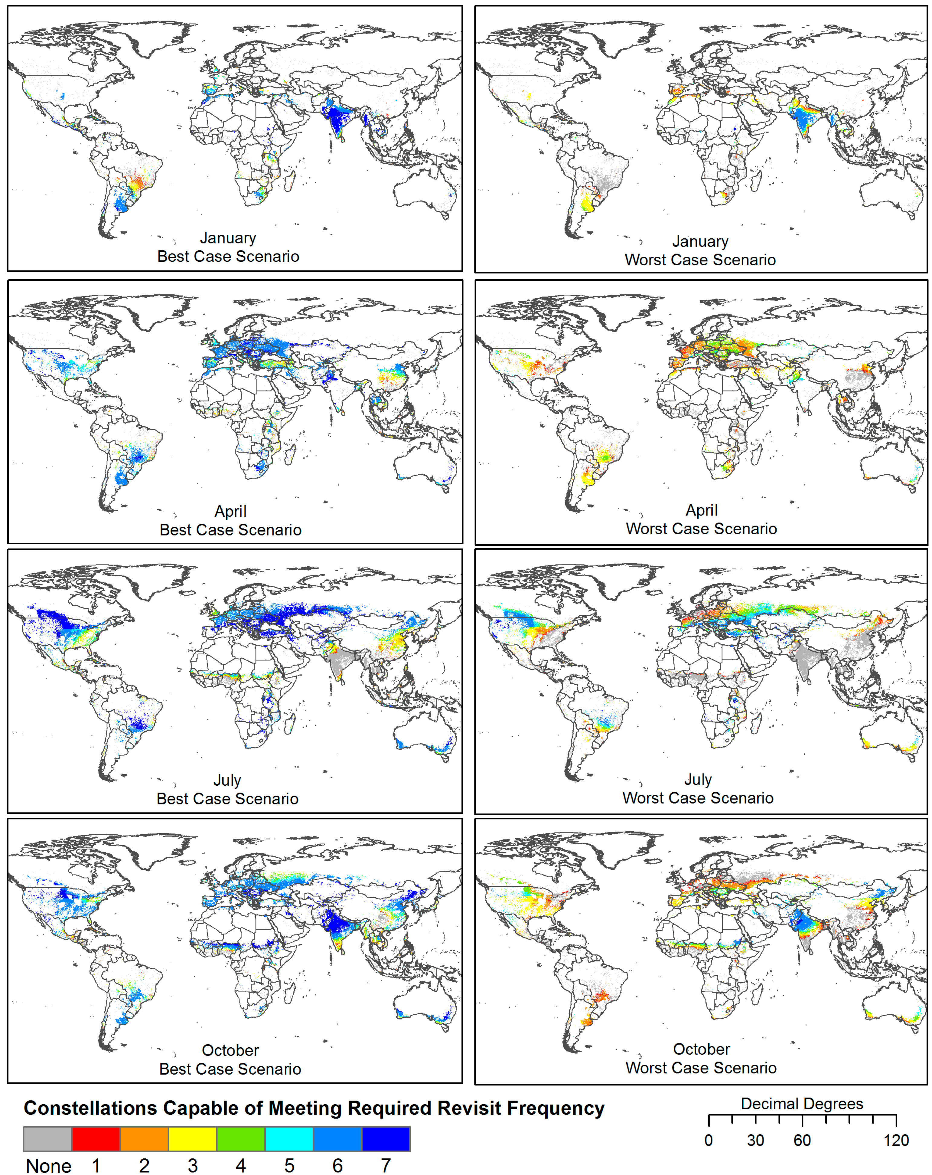
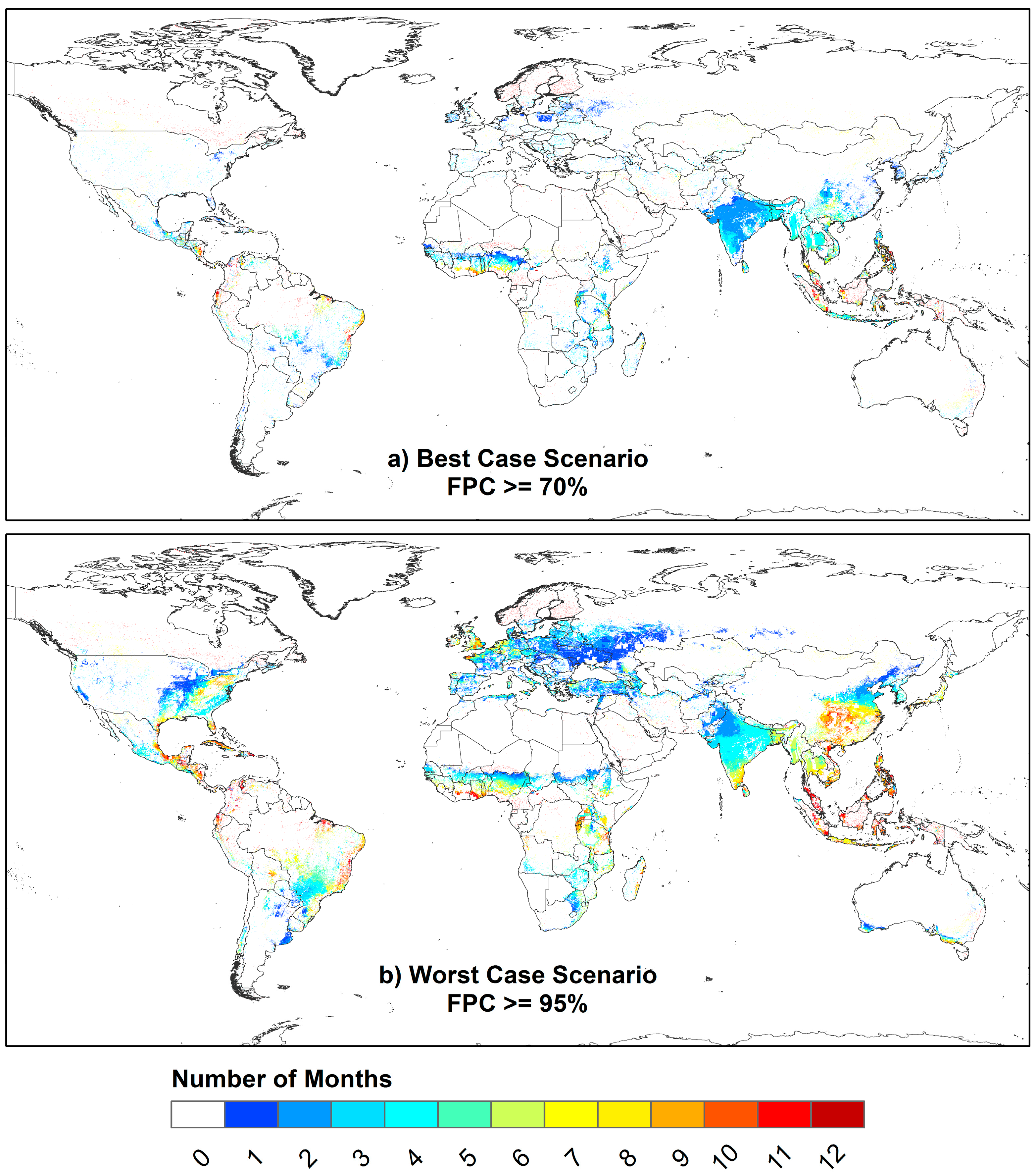
3.2. Persistently Cloudy Areas: Where Requirements Are Unmet

As seen in Figure 2, there are a number of cells/times of year shown in gray (with value “0”) for which none of the analyzed hypothetical constellations of polar-orbiting optical sensors have a combined revisit capability frequent enough to meet a reasonably cloud free requirement within 8 days. Requirement #6 in the GEOGLAM table (Table 1) states that moderate resolution microwave SAR data are required every 8 days in “persistently cloudy areas” (including/in addition to rice cultivating areas), which are defined herein as those areas and times of year which require a revisit in order to yield a reasonably clear view that is more frequent than our current/planned moderate resolution polar orbiting optical missions are capable of delivering. SAR data are not the only alternative—for example, data from geostationary satellites with multiple observations per day have been used, but at rather coarse spatial resolution [54]—but they are currently most broadly available non-optical moderate resolution type of data. Figure 6 shows the extent and number of months for which SAR data may be required for both scenarios examined.
Figure 6. The number of months throughout the agricultural growing season for which an 8 day requirement cannot be met by any of the seven moderate resolution polar-orbiting optical constellations evaluated, for the best case scenario (mode revisit vs. requirement for views at least 70% clear (a, top); and worst case scenario (mode revisit vs. requirement for views at least 95% clear (b, bottom). These areas are too persistently and pervasively cloudy for these systems, and as such, alternatives for monitoring—principally, SAR data (as in Table 1, Requirement #6), alone or fused with optical data should be considered.
Remotesensing 07 01482 g006
In the best case, very few areas (concentrated in Southeast Asia, West Africa (Gulf of Guinea), and parts of Eastern Europe and the Equatorial Americas) require microwave data for more than 3–4 months, with the majority of areas requiring SAR data for 0–2 months. The extreme cloud cover seasonality present in the Indian Summer Monsoon areas—very consistently and pervasively cloudy in June–September; very low cloud cover occultation in October-March, as seen in Figure 5—means that regardless of the cloud cover threshold, alternatives or supplements to optical data are required during those periods. A similar situation is apparent in the Gulf of Guinea, where in both scenarios, cloud cover is so pervasive during portions of the year that not even the 70% cloud free threshold can be satisfied by the constellations analyzed herein. Meanwhile, in the worst case scenario, the extent of necessary SAR data is expanded both in space and time, with many areas throughout the world requiring more than six months of SAR data. This highlights the potential value of microwave SAR data in a global agricultural monitoring system.

4. Discussion

There are three primary insights gained from this analysis. First, it is possible in many areas and periods of the year to meet the required revisit frequency with one or more of these proposed constellations, regardless of cloud cover threshold. However, it certainly necessitates a constellation beyond that which is currently freely available (Constellation #7), or these data must be supplemented in other areas/times of year by non-optical data, or data with even less strict cloud thresholds. By adding an additional instrument to the Constellation #7 (e.g., Sentinel-2A in Constellation #6; Resourcesat-2 in Constellation #3), success rates are increased in both scenarios, in virtually all regions. As agricultural monitoring applications increasingly rely upon daily to approximately weekly data, this is an important point for space agencies to consider in the development of future observatories or in developing inter-space agency collaboration. Further, the addition of Resourcesat-2 in Constellation #3 has a greater impact upon success rate than does the addition of Sentinel-2A alone (Constellation #6)—a jump from 12%–32% (Constellation #7, only L7 + L8) to 63%–87% (adding R2) versus 44%–67% (adding S2A) in the best case, and a jump from practically 0% in all months to 27%–49% versus 0%–18% in the worst case. In fact, R2 has the largest effect on increasing revisit frequency of any single satellite analyzed herein due to its very wide swath, albeit with a relatively lower spatial resolution (55 m). What these points suggest is that sensor architecture and alternative designs can and should be considered in the future, although this should be weighed against other factors such as the ground distortion at the edge of wide swath [55].
Second, loosening the definition of “reasonably” cloud free, as exemplified in the FPC ≥ 70% case, provides a promising outlook for the capabilities of our current and near-term moderate resolution optical instruments for many areas throughout the growing season. Areas wherein virtually clear views (e.g., 95% clear) are not probable, but at least one constellation is capable of yielding a view that is at least 70% clear, are good candidates for an image compositing approach, although it should be noted that this approach may underestimate the impacts of cloud cover as well as miss changes in crop condition and progress during the compositing period ([1,54,56]).
A third finding is that in both scenarios presented herein, for the 8 day reasonably clear data requirement, there are still areas and times for which no combination of our current and near-term moderate resolution optical instrumentation can yield a sufficient revisit frequency to overcome the pervasiveness of cloud cover. Space agencies can deploy a cadre of polar orbiting optical missions, but little difference will be made in areas/times that are frequently and pervasively occluded by clouds (e.g., South and Southeast Asia during the Summer Monsoon). These areas, as illustrated by Figure 6, are poorly suited for polar orbiting optical imaging, and alternative data sources, particularly microwave SAR data on its own or in fusion with optical data, should be considered. If willing to accept optical data which are at least 70% clear, that leaves between 9%–29% percent of 0.05° cells globally, depending on month, which can be characterized as requiring microwave SAR. However, if cells at least 95% clear are required, this leaves between 40%–58% of cells worldwide, a considerable quantity pointing at the value of further investing in research related to using data from alternatives to polar orbiting optical instruments.

Considerations and Limitations

There are a few caveats to consider in this analysis. First, pinning down the exact combined revisit frequency for each constellation is very challenging due to the repeat cycles of each component mission being out of sync with one another. For example, if there are 80 revisits within 120 days, it can only be said that the average combined revisit frequency is 1.5 days, although revisits may have actually alternated between 1 and 2 days apart. All of the satellites discussed herein are sun-synchronous with overpass times at (or projected to be at) 10:30 am, and so a revisit of 1.5 days is actually impossible. How precisely this impacts the success rate and merits further research and is beyond the scope of this analysis.
Further, the cloud data used in this analysis are natively at 1 km [57], scaled up as percentage of 1 km pixels which are cloudy within a 0.05° cell [50]. It makes no difference what percentage within the initial 1 km pixel is cloudy, so long as enough cloud is present for cloud detection to occur for that pixel. The impact of this sub-MODIS pixel level cloudiness on true percentage cloudy/clear at 0.05° is unknown.
Finally, it is worth noting that Landsat 7 has had a scan-line corrector (SLC) mirror failure since 2003, resulting in the absence of a considerable amount of data (22%) in stripes throughout the scene [58]. The remaining data are still valuable and usable [59], but this will impact the apparent revisit frequency, because even if the data are acquired (which is not a certitude, as systematic acquisitions are only planned for S2A + S2B), 22% of data will be missing from each L7 acquisition.

5. Conclusions and Future Research

The analysis presented herein shows the strength of combining multiple satellite missions to form an imaging constellation. Combining missions from two or three different space agencies leads to greatly improved revisit frequencies and an improvement in our ability to meet our EO requirements for global agricultural monitoring, although key gaps exist in pervasively and persistently cloudy regions. The extent and severity of these gaps in capability depend largely on the degree of acceptable cloud cover, and as such, research to pinpoint the precise definition of “reasonable” cloud cover for each agricultural monitoring application should be prioritized.
Future research should continue the investigation initiated by Gao et al. (2006) [60] regarding the utility of a moderate resolution MODIS-type system (with daily or even twice daily revisit capability) for meeting EO requirements for agriculture and other societal benefit areas. Such a revisit frequency could prove particularly useful for crop condition monitoring and yield forecasting with their reliance on frequent data, but it is possible that an investment in such a system would experience diminishing marginal returns due to persistent cloud cover, as exemplified by some areas/periods in the present analysis. For this reason, an increased investment in SAR systems and related algorithm development would be well-placed, as would a continued focus on SAR-optical data fusion [53,61,62,63,64,65,66].
Lastly, it is important to reiterate that an acquisition opportunity, as shown in this analysis, is just that—An opportunity, but not a fait accompli, in terms of acquisition or in terms of data availability. To date, agricultural analysts in many parts of the world have been hesitant to rely more fully upon a remote sensing based monitoring system due to concerns about data access, availability, interoperability, and continuity. Systematic acquisitions over actively cropped agricultural areas as well as a policy which guarantees continuous access to high quality, interoperable data are essential in the effort to meet EO requirements for agricultural monitoring [67].

Supplementary Files

Supplementary File 1

Acknowledgments

The authors would like to acknowledge Paul Kessler and Shaun Deacon in the CEOS Systems Engineering office for their assistance with the COVE simulation. We thank the CEOS Ad Hoc Team for GEOGLAM for their contributions in the development of the EO data requirements table. We thank Eric Vermote (NASA-GSFC), Samuel Goward (UMD) and Jeffrey Masek (NASA-GSFC) for their feedback and guidance. Finally, the authors would like to acknowledge the NASA Earth and Space Science Fellowship (NNX11AL56H) and NASA Applied Sciences (NNX1AQ79G) for their support of this work.

Author Contributions

Alyssa K. Whitcraft designed the research, performed the comparisons, analyzed the results, and drafted the manuscript. Together with Inbal Becker-Reshef and Brian D. Killough, she also selected the missions for inclusion in the development of hypothetical constellations. Brian D. Killough supervised the analysis run within COVE. All four authors revised the manuscript and contributed to the discussion, implications, future research, and conclusions.

Conflicts of Interest

The authors declare no conflict of interest.

References

  1. Whitcraft, A.K.; Becker-Reshef, I.; Justice, C. A Framework for Defining Spatially Explicit Earth Observation Requirements for a Global Agricultural Monitoring Initiative (GEOGLAM). Remote Sens. 2015, 7, 1461–1481. [Google Scholar] [CrossRef]
  2. Justice, C.O.; Vermote, E.; Privette, J.; Sei, A. The evolution of US moderate resolution optical land remote sensing from AVHRR to VIIRS. In Land Remote Sensing and Global Environmental Change; Springer: Berlin, Germany, 2011; pp. 781–806. [Google Scholar]
  3. Justice, C.O.; Vermote, E.; Townshend, J.R.G.; DeFries, R.; Roy, D.P.; Hall, D.K.; Salomonson, V.V.; Privette, J.L.; Riggs, G.; Strahler, A.; et al. The Moderate Resolution Imaging Spectroradiometer (MODIS): land remote sensing for global change research. IEEE Trans. Geosci. Remote Sens. 1998, 36, 1228–1249. [Google Scholar] [CrossRef]
  4. Goward, S.N.; Arvidson, T.; Williams, D.L.; Irish, R.; Irons, J.R. Moderate Spatial Resolution Optical Sensors; SAGE Publications Ltd.: London, UK, 2009. [Google Scholar]
  5. Goward, S.; Williams, D.; Arvidson, T.; Irons, J. The future of landsat-class remote sensing. In Land Remote Sensing and Global Environmental Change; Springer: Berlin, Germany, 2011; pp. 807–834. [Google Scholar]
  6. Goward, S.; Chander, G.; Pagnutti, M.; Marx, A.; Ryan, R.; Thomas, N.; Tetrault, R. Complementarity of ResourceSat-1 AWiFS and Landsat TM/ETM+ sensors. Remote Sens. Environ. 2012, 123, 41–56. [Google Scholar] [CrossRef]
  7. Wulder, M.A.; Masek, J.G.; Cohen, W.B.; Loveland, T.R.; Woodcock, C.E. Opening the archive: How free data has enabled the science and monitoring promise of Landsat. Remote Sens. Environ. 2012, 122, 2–10. [Google Scholar] [CrossRef]
  8. Roy, D.P.; Wulder, M.A.; Loveland, T.R.; Allen, R.G.; Anderson, M.C.; Helder, D.; Irons, J.R.; Johnson, D.M.; Kennedy, R.; Scambos, T.A. Landsat-8: Science and product vision for terrestrial global change research. Remote Sens. Environ. 2014, 145, 154–172. [Google Scholar] [CrossRef]
  9. Gong, P.; Wang, J.; Yu, L.; Zhao, Y.; Zhao, Y.; Liang, L.; Niu, Z.; Huang, X.; Fu, H.; Liu, S.; et al. Finer resolution observation and monitoring of global land cover: First mapping results with Landsat TM and ETM+ data. Int. J. Remote Sens. 2013, 34, 2607–2654. [Google Scholar] [CrossRef]
  10. Hansen, M.C.; Potapov, P.V.; Moore, R.; Hancher, M.; Turubanova, S.A.; Tyukavina, A.; Thau, D.; Stehman, S.V.; Goetz, S.J.; Loveland, T.R. High-Resolution global maps of 21st-century forest cover change. Science 2013, 342, 850–853. [Google Scholar] [CrossRef] [PubMed]
  11. Johnson, D.M.; Mueller, R. The 2009 cropland data layer. Photogramm. Eng. Remote Sens. 2010, 76, 1201–1205. [Google Scholar]
  12. Roy, D.P.; Ju, J.; Kline, K.; Scaramuzza, P.L.; Kovalskyy, V.; Hansen, M.; Loveland, T.R.; Vermote, E.; Zhang, C. Web-enabled Landsat Data (WELD): Landsat ETM+ composited mosaics of the conterminous United States. Remote Sens. Environ. 2010, 114, 35–49. [Google Scholar] [CrossRef]
  13. Yu, L.; Wang, J.; Clinton, N.; Xin, Q.; Zhong, L.; Chen, Y.; Gong, P. FROM-GC: 30 m global cropland extent derived through multisource data integration. Int. J. Digit. Earth 2013, 6, 521–533. [Google Scholar] [CrossRef]
  14. Justice, C.O.; Román, M.O.; Csiszar, I.; Vermote, E.F.; Wolfe, R.E.; Hook, S.J.; Friedl, M.; Wang, Z.; Schaaf, C.B.; Miura, T. Land and cryosphere products from Suomi NPP VIIRS: Overview and status. J. Geophys. Res.: Atmos. 2013, 118, 9753–9765. [Google Scholar] [CrossRef]
  15. Homer, C.; Dewitz, J.; Fry, J.; Coan, M.; Hossain, N.; Larson, C.; Herold, N.; McKerrow, A.; VanDriel, J.N.; Wickham, J. Completion of the 2001 national land cover database for the counterminous United States. Photogramm. Eng. Remote Sens. 2007, 73, 337–341. [Google Scholar]
  16. Skole, D.; Tucker, C. Tropical deforestation and habitat fragmentation in the Amazon. Satellite data from 1978 to 1988. Science 1993, 260, 1905–1910. [Google Scholar] [CrossRef] [PubMed]
  17. Vogelmann, J.E.; Howard, S.M.; Yang, L.; Larson, C.R.; Wylie, B.K.; Van Driel, N. Completion of the 1990s national land cover data set for the conterminous United States from Landsat thematic mapper data and ancillary data sources. Photogramm. Eng. Remote Sens. 2001, 67, 650–662. [Google Scholar]
  18. Wulder, M.A.; White, J.C.; Goward, S.N.; Masek, J.G.; Irons, J.R.; Herold, M.; Cohen, W.B.; Loveland, T.R.; Woodcock, C.E. Landsat continuity: Issues and opportunities for land cover monitoring. Remote Sens. Environ. 2008, 112, 955–969. [Google Scholar] [CrossRef]
  19. Li, Q.; Wu, B. Accuracy assessment of planted area proportion using Landsat TM imagery. J. Remote Sens. 2004, 8, 581–587. [Google Scholar]
  20. Underwood, C.; Machin, S.; Stephens, P.; Hodgson, D.; da Silva Curiel, A.; Sweeting, M. Evaluation of the utility of the disaster monitoring constellation in support of earth observation applications. In Proceedings of Small Satellites for Earth Observation: Selected Proceedings of the 5th International Symposium of the International Academy of Astronautics, Berlin, Germany, 4–8 April 2005.
  21. GEO-GEOGLAM (Global Agirculture Monitoring Initiative). Available online: http://www.earthobservations.org/geoglam_cop.php (accessed on 4 November 2014).
  22. Parihar, J.S.; Oza, M.P. FASAL: An integrated approach for crop assessment and production forecasting. Proc. SPIE 2006, 6411. [Google Scholar] [CrossRef]
  23. Wu, B.; Meng, J.; Li, Q.; Yan, N.; Du, X.; Zhang, M. Remote sensing-based global crop monitoring: experiences with China’s Crop Watch system. Int. J. Digit. Earth 2014, 7, 113–137. [Google Scholar] [CrossRef]
  24. Baruth, B.; Royer, A.; Klisch, A.; Genovese, G. The use of remote sensing within the MARS crop yield monitoring system of the European commission. Int. Arch. Photogramm. Remote Sens. Spat. Inf. Sci. 2008, 37, 935–940. [Google Scholar]
  25. Genovese, G.; Vignolles, C.; Nègre, T.; Passera, G. A methodology for a combined use of normalised difference vegetation index and CORINE land cover data for crop yield monitoring and forecasting. A case study on Spain. Agronomie 2001, 21, 91–111. [Google Scholar] [CrossRef]
  26. Allen, R.; Hanuschak, G.; Craig, M. History of remote Sensing for crop acreage in USDA’s National Agricultural Statistics Service; NASS: Washington, DC, USA, 2002. [Google Scholar]
  27. Duveiller, G.; Defourny, P.; Gérard, B. A method to determine the appropriate spatial resolution required for monitoring crop growth in a given agricultural landscape. In Proceedings of 2008 IEEE International Geoscience and Remote Sensing Symposium, IGARSS 2008, Boston, MA, USA, 7–11 July 2008; pp. 562–565.
  28. Developing a Strategy for Global Agricultural Monitoring in the framework of Group on Earth Observations (GEO) Workshop Report. Available online: http://www.fao.org/gtos/igol/docs/meeting-reports/07-geo-ag0703-workshop-report-nov07.pdf (accessed on 27 January 2015).
  29. Committee on Earth Observation Satellites. CEOS Acquisition Strategy for GEOGLAM Phase 1. Available online: http://ceos.org/images/Plenary2013/25-CEOS_Acquisition_Strategy_for_GEOGLAM_Phase-1_v1-0.pdf (accessed on 14 November 2014).
  30. Landsat. Available online: http://landsat.usgs.gov/index.php (accessed on 14 November 2014).
  31. Fosnight, E.; USGS/EROS Data Center, Sioux Falls, SD, USA. Personal Communication regarding Landsat 7&8 Acquisitions, 2014.
  32. Arvidson, T.; Gasch, J.; Goward, S.N. Pleasing all of the people most of the time: Planning Landsat 7 acquisitions for the US archive. In Proceedings of Pecora 14 - Land Satellite Information III: Demonstrating the Value of Satellite Imagery, ASPRS, Denver, CO, USA, 6–10 December 1999; pp. 154–162.
  33. Arvidson, T.; Gasch, J.; Goward, S.N. Landsat 7’s long-term acquisition plan—An innovative approach to building a global imagery archive. Remote Sens. Environ. 2001, 78, 13–26. [Google Scholar] [CrossRef]
  34. Arvidson, T.; Goward, S.; Gasch, J.; Williams, D. Landsat-7 long-term acquisition plan: Development and validation. Photogramm. Eng. Remote Sens. 2006, 72, 1137–1146. [Google Scholar] [CrossRef]
  35. Welcome to ISRO : Satellites : Earth Observation Satellite : RESOURCESAT-2. Available online: http://www.isro.org/satellites/resourcesat-2.aspx (accessed on 4 November 2014).
  36. Boryan, C.; Craig, M. Multiresolution Landsat TM and AWiFS sensor assessment for crop area estimation in Nebraska. In Proceedings of Pecora 16 “Global Priorities in Land Remote Sensing”, Sioux Falls, SD, USA, 23–27 October 2005; pp. 22–27.
  37. Sentinel-2 / Copernicus / Observing the Earth / Our Activities / ESA. Available online: http://www.esa.int/Our_Activities/Observing_the_Earth/Copernicus/Sentinel-2 (accessed on 4 November 2014).
  38. Drusch, M.; Del Bello, U.; Carlier, S.; Colin, O.; Fernandez, V.; Gascon, F.; Hoersch, B.; Isola, C.; Laberinti, P.; Martimort, P.; et al. Sentinel-2: ESA’s optical high-resolution mission for GMES operational services. Remote Sens. Environ. 2012, 120, 25–36. [Google Scholar] [CrossRef]
  39. ESA–NASA collaboration fosters comparable land imagery. Available online: http://www.esa.int/Our_Activities/Observing_the_Earth/Copernicus/ESA_NASA_collaboration_fosters_comparable_land_imagery (accessed on 10 September 2014).
  40. Anderson, M.C.; Hain, C.; Wardlow, B.; Pimstein, A.; Mecikalski, J.R.; Kustas, W.P. Evaluation of drought indices based on thermal remote sensing of evapotranspiration over the continental United States. J. Clim. 2011, 24, 2025–2044. [Google Scholar] [CrossRef]
  41. Hain, C.R.; Crow, W.T.; Mecikalski, J.R.; Anderson, M.C.; Holmes, T. An intercomparison of available soil moisture estimates from thermal infrared and passive microwave remote sensing and land surface modeling. J. Geophys. Res.: Atmos. 2011, 116, 1–18. [Google Scholar] [CrossRef]
  42. Tomlinson, C.J.; Chapman, L.; Thornes, J.E.; Baker, C. Remote sensing land surface temperature for meteorology and climatology: A review. Meteorol. Appl. 2011, 18, 296–306. [Google Scholar]
  43. Weng, Q.; Fu, P.; Gao, F. Generating daily land surface temperature at Landsat resolution by fusing Landsat and MODIS data. Remote Sens. Environ. 2014, 145, 55–67. [Google Scholar] [CrossRef]
  44. Frey, R.A.; Ackerman, S.A.; Liu, Y.; Strabala, K.I.; Zhang, H.; Key, J.R.; Wang, X. Cloud detection with MODIS. Part I: Improvements in the MODIS cloud mask for Collection 5. J. Atmos. Ocean. Technol. 2008, 25, 1057–1072. [Google Scholar] [CrossRef]
  45. Johnson, D.M. An assessment of pre-and within-season remotely sensed variables for forecasting corn and soybean yields in the United States. Remote Sens. Environ. 2014, 141, 116–128. [Google Scholar] [CrossRef]
  46. Kessler, P.D.; Killough, B.D.; Gowda, S.; Williams, B.R.; Chander, G.; Qu, M. CEOS Visualization Environment (COVE) Tool for Intercalibration of Satellite Instruments. IEEE Trans. Geosci. Remote Sens. 2013, 51, 1081–1087. [Google Scholar] [CrossRef]
  47. Chander, G.; Killough, B.; Gowda, S. An overview of the web-based Google Earth coincident imaging tool. In proceedings of 2010 IEEE International Geoscience and Remote Sensing Symposium (IGARSS), 25–30 July 2010; pp. 1679–1682.
  48. Whitcraft, A.K.; Becker-Reshef, I.; Justice, C.O. Agricultural growing season calendars derived from MODIS surface reflectance. Int. J. Digit. Earth 2014. [Google Scholar] [CrossRef]
  49. Fritz, S.; See, L.; McCallum, I.; You, L.; Bun, A.; Moltchanova, E.; Duerauer, M.; Albrecht, F.; Schill, C.; Perger, C.; et al. Mapping global cropland and field size. Glob. Change Biol. 2015. [Google Scholar] [CrossRef] [Green Version]
  50. Whitcraft, A.K.; Vermote, E.F.; Becker-Reshef, I.; Justice, C.O. Cloud cover throughout the agricultural growing season: Impacts on passive optical earth observations. Remote Sens. Environ. 2015, 156, 438–447. [Google Scholar] [CrossRef]
  51. Takashima, S.; Oyoshi, K.; Fukuda, T.; Okumura, T.; Tomiyama, N.; Nagano, T. Asia rice crop monitoring in GEO GLAM. In Proceedings of 2013 IEEE Second International Conference on Agro-Geoinformatics (Agro-Geoinformatics), Fairfax, VA, USA, 12–16 August 2013; pp. 398–401.
  52. Takashima, S.S.; Oyoshi, K.; Okumura, T.; Tomiyama, N.; Rakwatin, P. Rice crop yield monitoring system prototyping and its evaluation result. In Proceedings of the 2012 IEEE First International Conference on Agro-Geoinformatics (Agro-Geoinformatics), Shanghai, China, 2–4 August 2012; pp. 1–4.
  53. McNairn, H.; Champagne, C.; Shang, J.; Holmstrom, D.; Reichert, G. Integration of optical and Synthetic Aperture Radar (SAR) imagery for delivering operational annual crop inventories. ISPRS J. Photogramm. Remote Sens. 2009, 64, 434–449. [Google Scholar] [CrossRef]
  54. Duveiller, G.; López-Lozano, R.; Seguini, L.; Bojanowski, J.S.; Baruth, B. Optical remote sensing requirements for operational crop monitoring and yield forecasting in Europe. In Proceedings of Sentinel-3 OLCI/SLSTR and MERIS/(A) ATSR Workshop, ESA SP-711, Frascati, Italy, 15–19 October 2012.
  55. Verma, N.; Garg, P.; Garg, R. Evaluation of geometric properties of AWiFS images: A comparative study. Geomat. Eng. 2009. Available online: http://www.csre.iitb.ac.in/~csre/conf/wp-content/uploads/fullpapers/OS1/OS1_1.pdf (accessed on 28 January 2015).
  56. Roy, D.P.; Lewis, P.; Schaaf, C.B.; Devadiga, S.; Boschetti, L. The global impact of clouds on the production of MODIS bidirectional reflectance model-based composites for terrestrial monitoring. Geosci. Remote Sens. Lett. 2006, 3, 452–456. [Google Scholar] [CrossRef]
  57. Vermote, E.F.; El Saleous, N.Z.; Justice, C.O. Atmospheric correction of MODIS data in the visible to middle infrared: first results. Remote Sens. Environ. 2002, 83, 97–111. [Google Scholar] [CrossRef]
  58. Scaramuzza, P.; Micijevic, E.; Chander, G. SLC gap-filled products phase one methodology. In Landsat Tech. Notes; 2004; pp. 1–5. Available online: http://landsat.usgs.gov/documents/SLC_Gap_Fill_Methodology.pdf (accessed on 28 January 2015). [Google Scholar]
  59. Maxwell, S.K.; Schmidt, G.L.; Storey, J.C. A multi-scale segmentation approach to filling gaps in Landsat ETM+ SLC-off images. Int. J. Remote Sens. 2007, 28, 5339–5356. [Google Scholar] [CrossRef]
  60. Gao, F.; Masek, J.; Schwaller, M.; Hall, F. On the blending of the Landsat and MODIS surface reflectance: Predicting daily Landsat surface reflectance. IEEE Trans. Geosci. Remote Sens. 2006, 44, 2207–2218. [Google Scholar] [CrossRef]
  61. Hong, G.; Zhang, A.; Zhou, F.; Brisco, B. Integration of optical and Synthetic Aperture Radar (SAR) images to differentiate grassland and alfalfa in Prairie area. Int. J. Appl. Earth Obs. Geoinf. 2014, 28, 12–19. [Google Scholar] [CrossRef]
  62. Kussul, N.; Skakun, S.; Shelestov, A.; Kravchenko, O.; Kussul, O. Crop classification in Ukraine using satellite optical and SAR images. Inf. Models Anal. 2012, 2, 118–122. [Google Scholar]
  63. Leichtle, T.; Schmitt, A.; Roth, A.; Schardt, M. On the capability of different SAR polarization combinations for agricultural monitoring. In Proceedings of the 2012 IEEE International Geoscience and Remote Sensing Symposium (IGARSS), Munich, Germany, 22–27 July 2012; pp. 3752–3755.
  64. McNairn, H.; Shang, J.; Champagne, C.; Jiao, X. TerraSAR-X and RADARSAT-2 for crop classification and acreage estimation. In Proceedings of the 2009 IEEE International Geoscience and Remote Sensing Symposium, IGARSS 2009, Cape Town, South Africa, 12–17 July 2009; pp. II-898–II-901.
  65. McNairn, H.; Shang, J.; Jiao, X.; Champagne, C. The contribution of ALOS PALSAR multipolarization and polarimetric data to crop classification. IEEE Trans. Geosci. Remote Sens. 2009, 47, 3981–3992. [Google Scholar] [CrossRef]
  66. Torbick, N.; Salas, W.; Xiao, X.; Ingraham, P.; Fearon, M.; Biradar, C.; Zhao, D.; Liu, Y.; Li, P.; Zhao, Y. Integrating SAR and optical imagery for regional mapping of paddy rice attributes in the Poyang Lake Watershed, China. Can. J. Remote Sens. 2011, 37, 17–26. [Google Scholar] [CrossRef]
  67. Atzberger, C. Advances in remote sensing of agriculture: Context description, existing operational monitoring systems and major information needs. Remote Sens. 2013, 5, 949–981. [Google Scholar] [CrossRef]

