
Time Series Analysis of Landslide Dynamics Using an Unmanned Aerial Vehicle (UAV)


Abstract
:
1. Introduction
2. Methodology
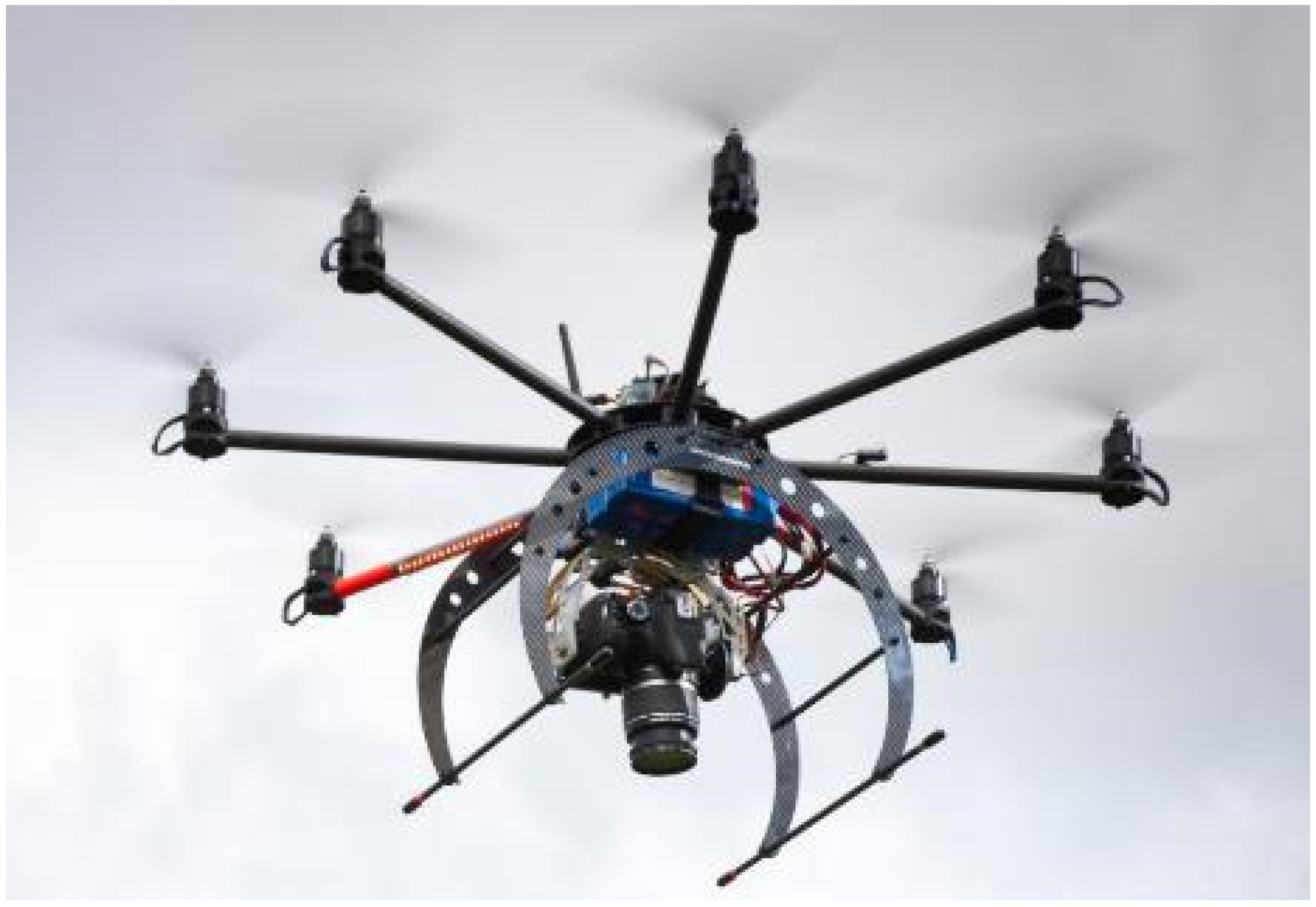
2.1. Platform

2.2. Sensor
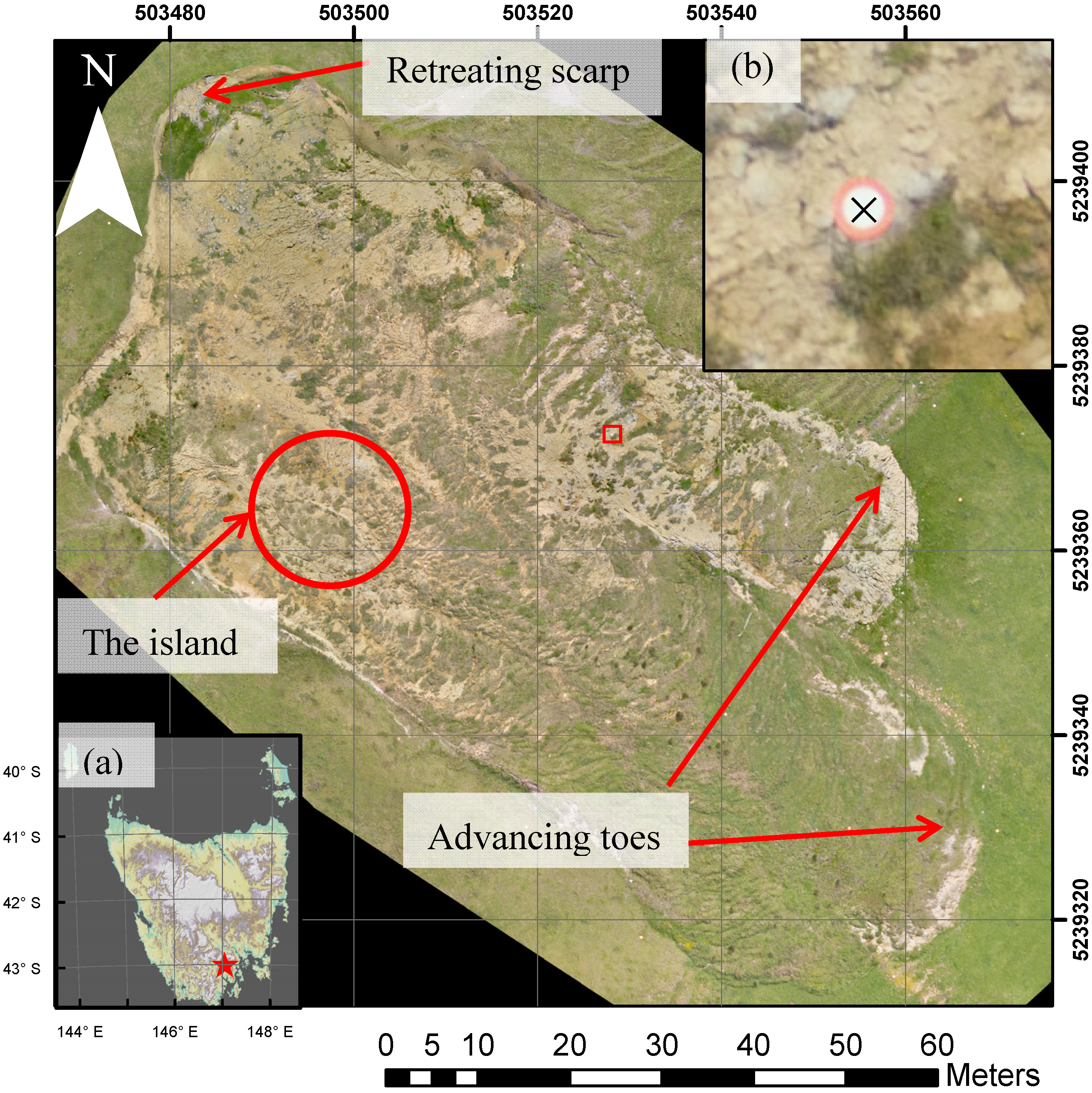
2.3. Field Site


| Survey Name | Date | Interval (Days) | Weather Conditions |
|---|---|---|---|
| 2010A | 20 July 2010 | - | Sunny, light winds |
| 2011A | 19 July 2011 | 364 | Overcast, light rain and wind |
| 2011B | 10 November 2011 | 114 | Sunny, moderate winds |
| 2012A | 27 July 2012 | 260 | Sunny, light winds |
| 2013A | 5 April 2013 | 252 | Sunny, moderate winds |
| 2013B | 29 July 2013 | 115 | Sunny, moderate winds |
| 2014A | 25 July 2014 | 361 | Sunny, no wind |
2.4. Three-Dimensional Model Generation
2.5. Alignment of Digital Surface Models
| DSM Pair | Prior to Offset Application | Offset Applied (m) | After Offset Application | ||
|---|---|---|---|---|---|
| Volume Difference (m3) | RMSE (m) | Volume Difference (m3) | RMSE (m) | ||
| 2010A–2011A | 153 | 0.109 | 0.10 | 114 | 0.077 |
| 2011A–2011B | 88 | 0.061 | 0.00 | 88 | 0.061 |
| 2011B–2012A | 98 | 0.074 | 0.00 | 98 | 0.074 |
| 2012A–2013A | 134 | 0.108 | 0.09 | 115 | 0.085 |
| 2013A–2013B | 148 | 0.101 | 0.13 | 102 | 0.087 |
| 2013B–2014A | 76 | 0.059 | 0.00 | 76 | 0.059 |
2.6. Measurement of Landslide Area and Volume Change
2.7. Tracking of Landslide Surface Movement
3. Results
3.1. Accuracy of DSMs and Orthophotos
| Name | Date | Number Photos Used in Model | GCPs | Checkpoints | XY RMSE (m) | Z RMSE (m) |
|---|---|---|---|---|---|---|
| 2010A | 20 July 2010 | 62 | 56 | 19 | 0.046 | 0.031 |
| 2011A | 19 July 2011 | 116 | 41 | 20 | 0.045 | 0.042 |
| 2011B | 10 November 2011 | 194 | 23 | 23 * | 0.021 | 0.025 |
| 2012A | 27 July 2012 | 170 | 66 | 17 | 0.047 | 0.039 |
| 2013A | 5 April 2013 | 179 | 29 | 22 | 0.058 | 0.078 |
| 2013B | 29 July 2013 | 241 | 23 | 21 | 0.076 | 0.090 |
| 2014A | 25 July 2014 | 415 | 16 | 10 | 0.031 | 0.031 |
3.2. Area and Slope Analysis

| Name | Total Area (m2) | Slope of Large Toe (Deg) | Slope of Small Toe (Deg) | Area of Toe Advance (m2) | Area of Scarp Retreat (m2) |
|---|---|---|---|---|---|
| 2010A | 4887 | 31.05 | 36.26 | - | - |
| 2011A | 5168 | 33.72 | 34.92 | 281 | - |
| 2011B | 5435 | 34.37 | 34.06 | 105 | 162 |
| 2012A | 5455 | 39.98 | 36.22 | 20 | - |
| 2013A | 5675 | 34.17 | 34.78 | 126 | 95 |
| 2013B | 5675 | 33.17 | 34.54 | - | - |
| 2014A | 5744 | 33.87 | 37.63 | 22 | 47 |
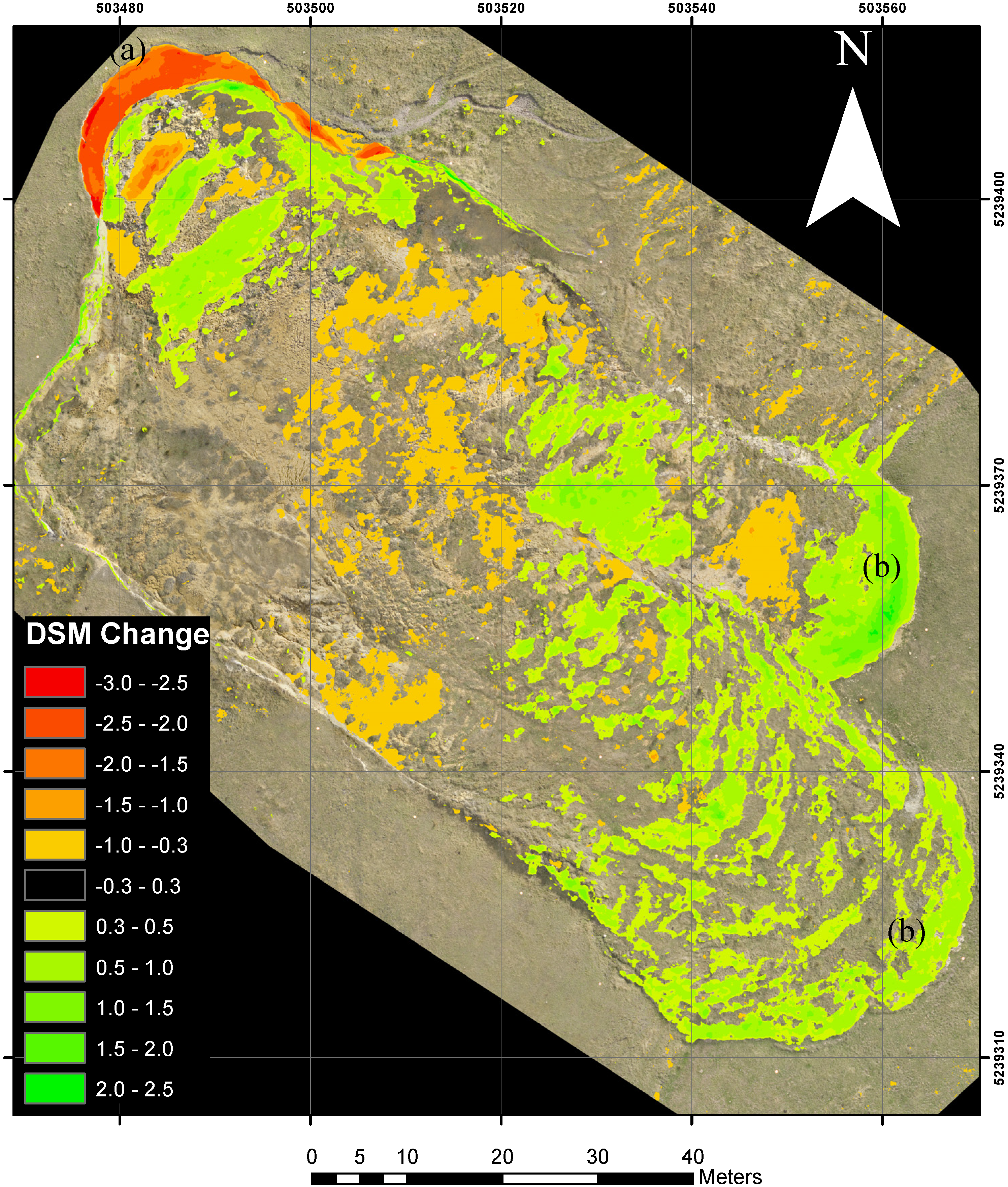
3.3. DSM Volumetric Changes
| Name | Toe Accumulation and Estimated Error (m3) | Loss above Toe and Estimated Error (m3) | Bulking Factor |
|---|---|---|---|
| 2010A → 2011A | 572 ± 24 | 340 ± 14 | 1.68 |
| 2011A → 2011B | 249 ± 21 | 124 ± 17 | 2.00 |
| 2011B → 2012A | 88 ± 19 | 24 ± 10 | 3.66 |
| 2012A → 2013A | 175 ± 21 | 41 ± 9 | 4.27 |
| 2013A → 2013B | no change | no change | - |
| 2013B → 2014A | 85 ± 17 | 22 ± 8 | 3.86 |

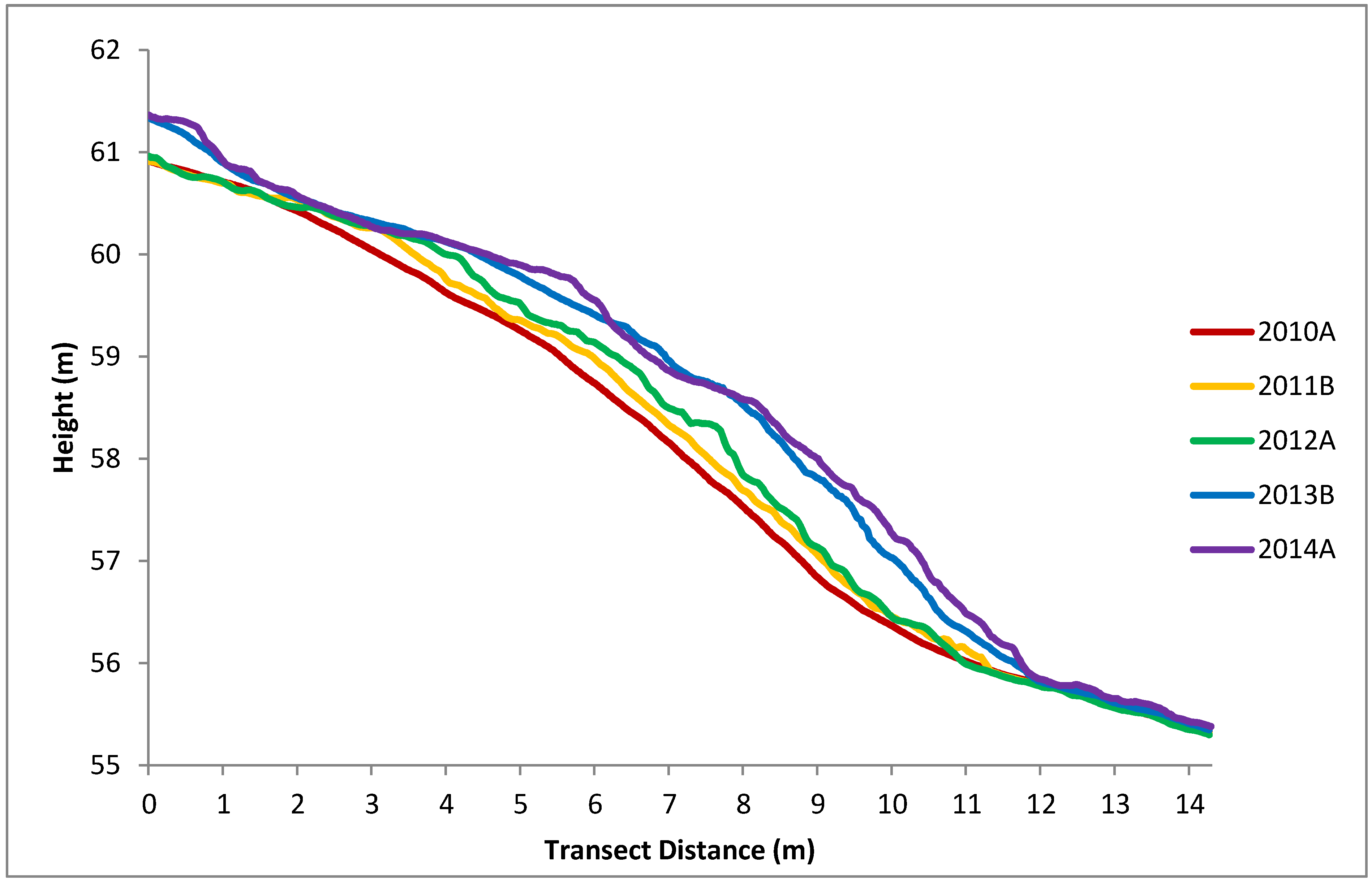
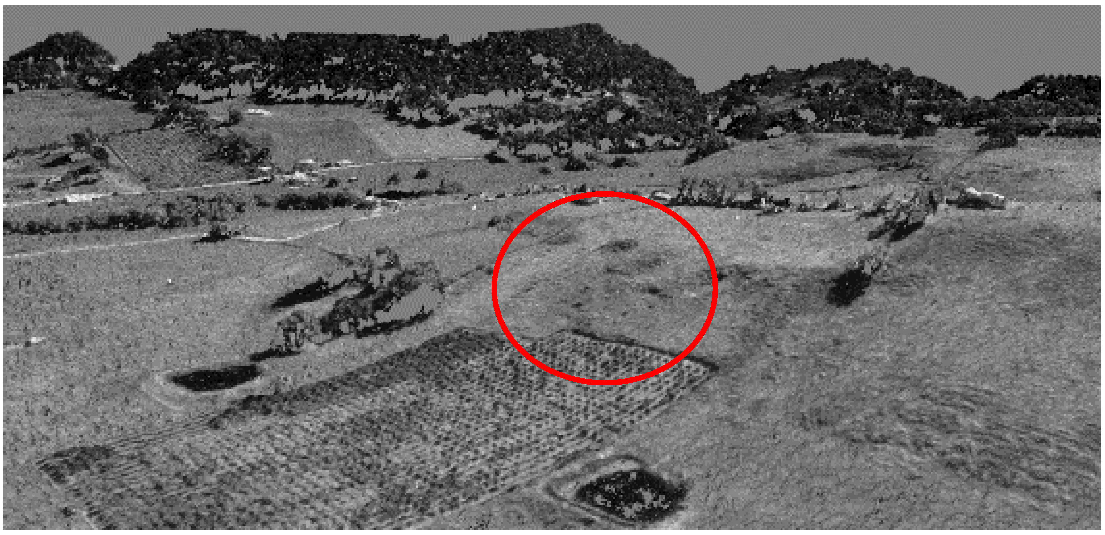
3.4. Historical DSM

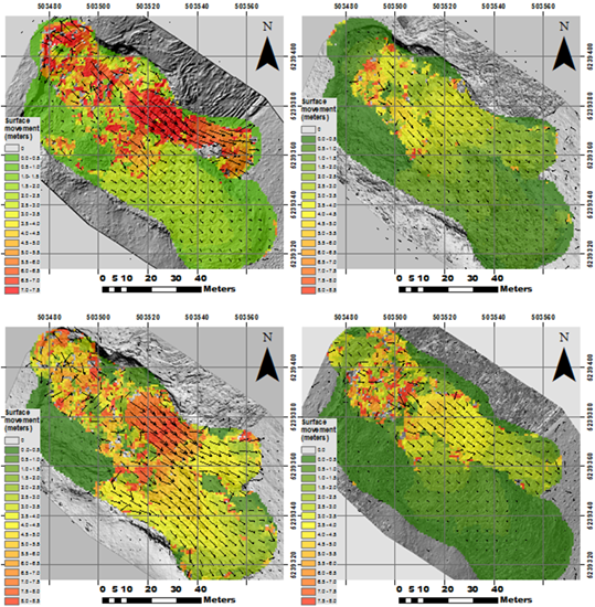
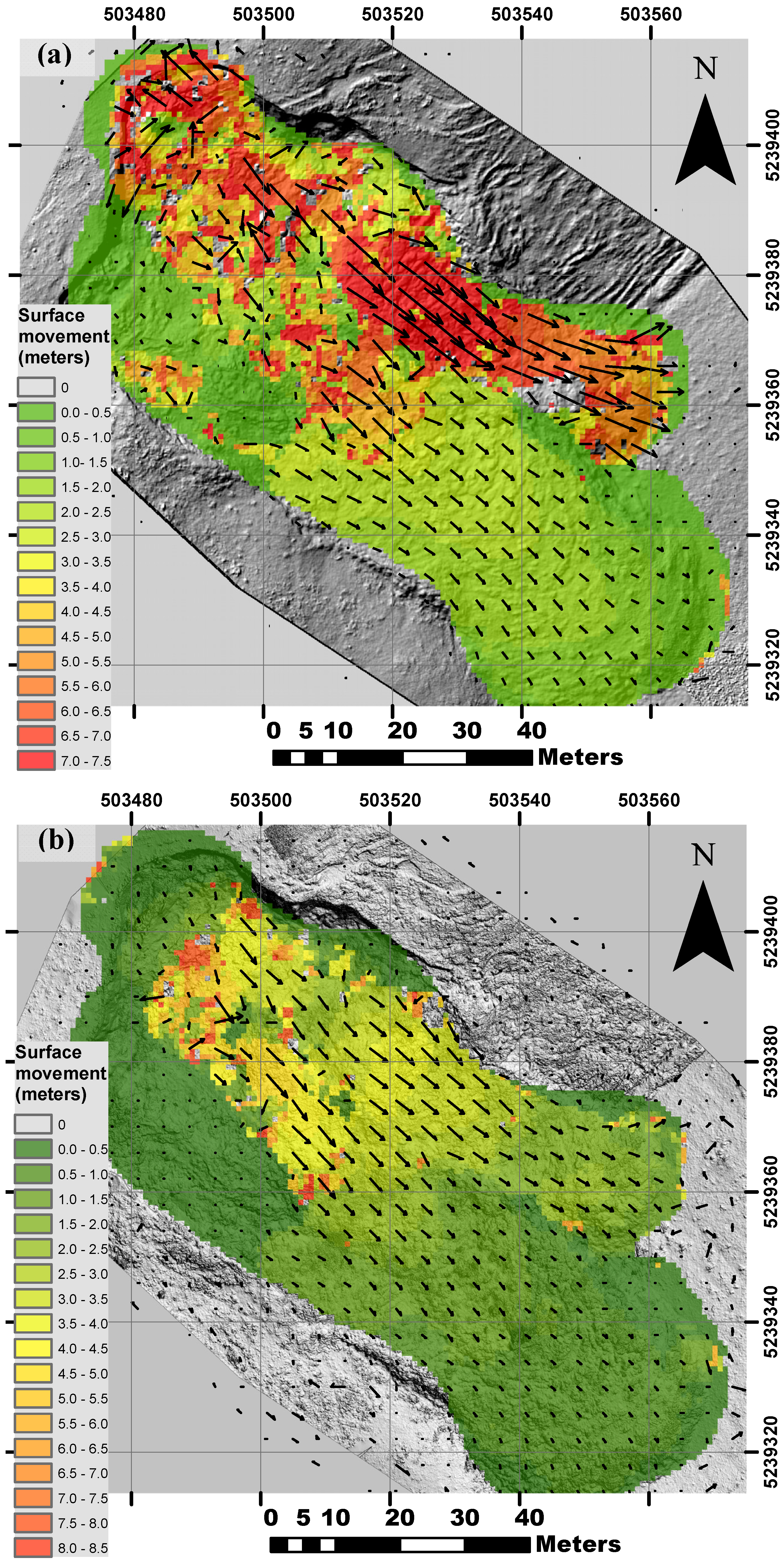
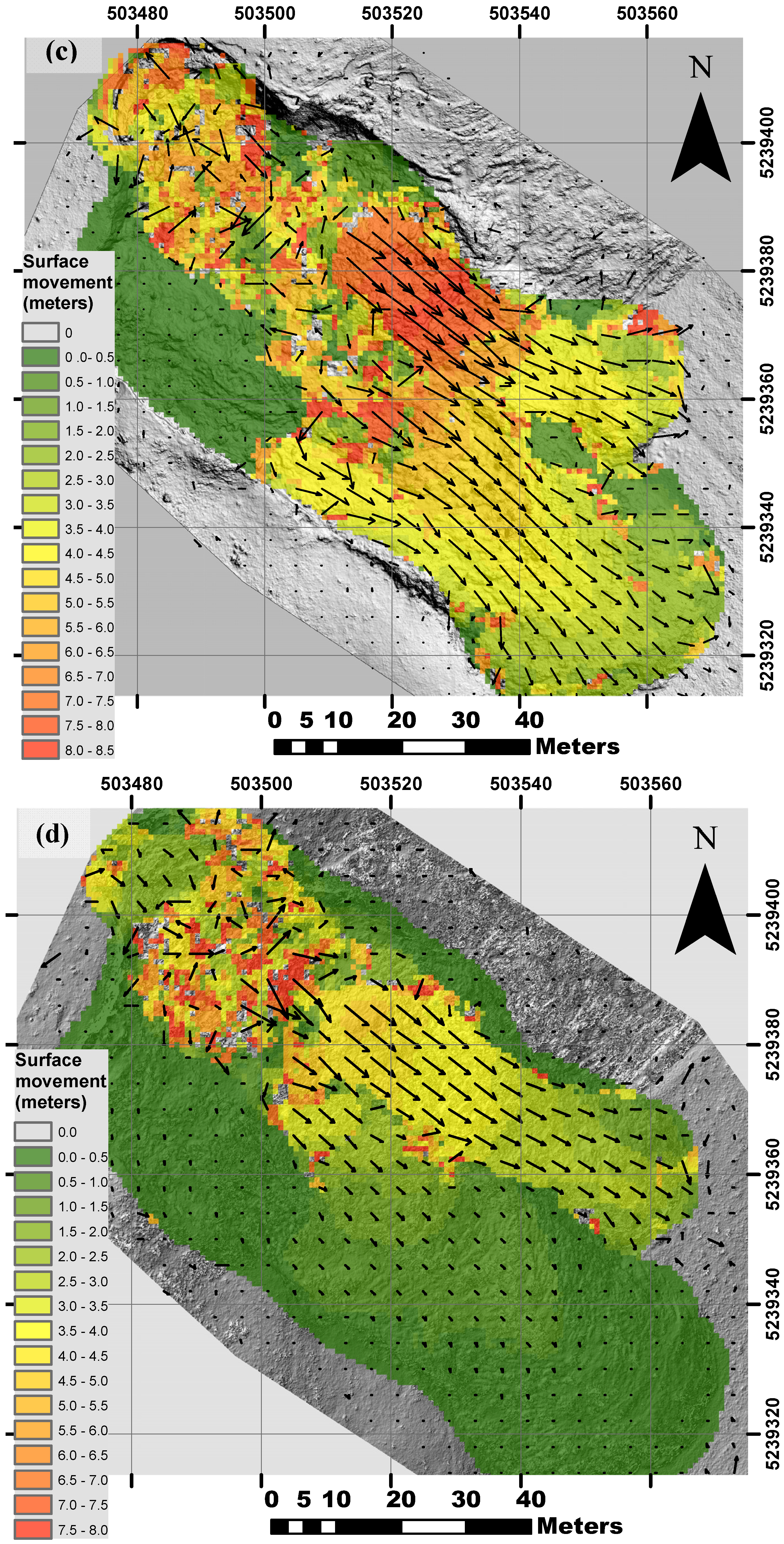
3.5. Surface Movement


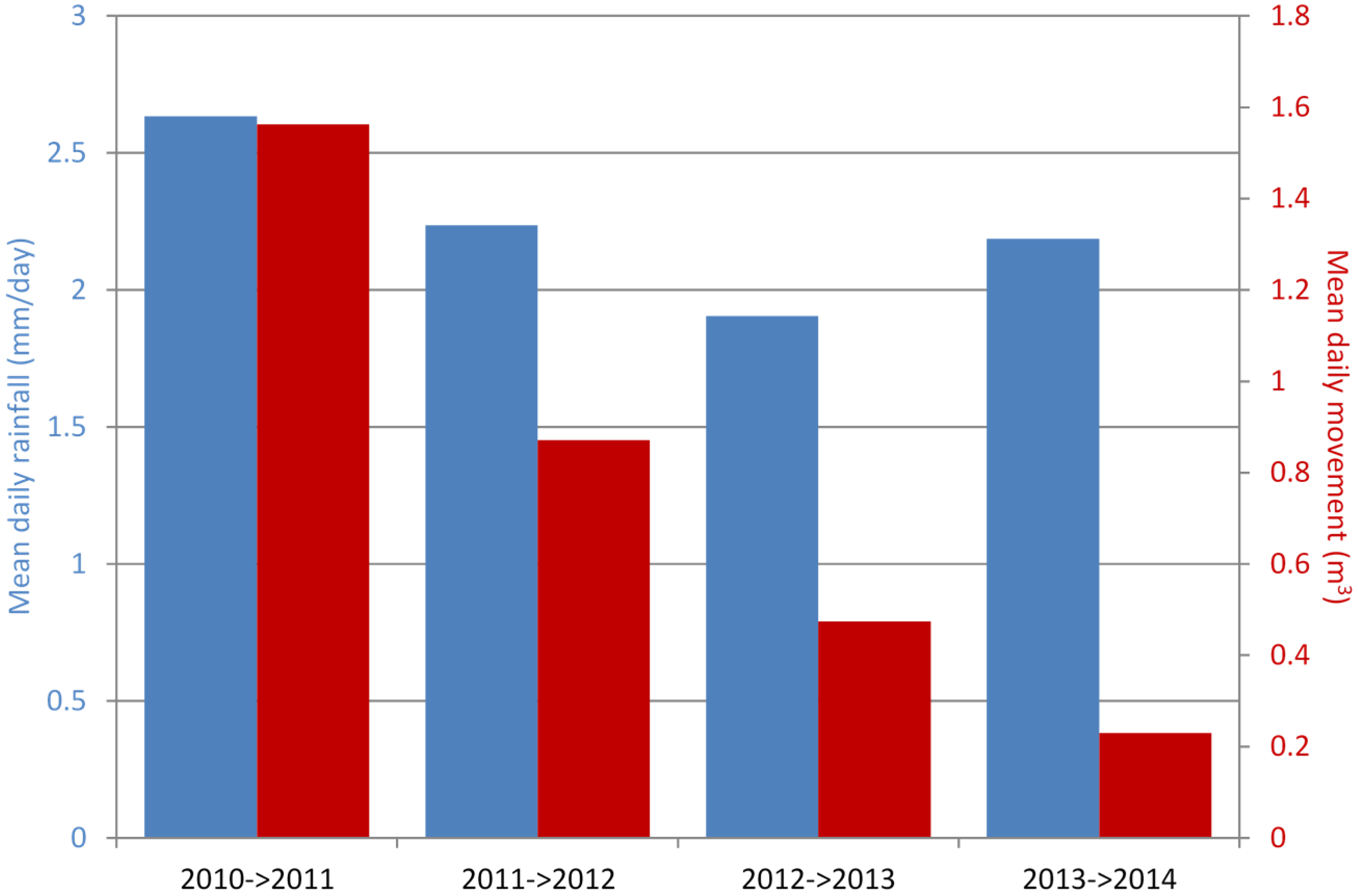
3.6. Comparison of Landslide Movement with Rainfall

4. Discussion
5. Conclusions
Acknowledgments
Author Contributions
Conflicts of Interest
References
- Schuster, R.L. Scoioeconomic significance of landslides. In Landslides—Investigation and Mitigation; Turner, A.K., Schuster, R.L., Eds.; National Research Council: Washington, DC, USA, 1996; pp. 12–35. [Google Scholar]
- Pesci, A.; Teza, G.; Casula, G.; Loddo, F.; De Martino, P.; Dolce, M.; Obrizzo, F.; Pingue, F. Multitemporal laser scanner-based observation of the Mt. Vesuvius crater: Characterization of overall geometry and recognition of landslide events. ISPRS J. Photogramm. Remote Sens. 2011, 66, 327–336. [Google Scholar] [CrossRef]
- Nadim, F.; Kjekstad, O.; Peduzzi, P.; Herold, C.; Jaedicke, C. Global landslide and avalanche hotspots. Landslides 2006, 3, 159–173. [Google Scholar] [CrossRef]
- Bell, R.; Petschko, H.; Rohrs, M.; Dix, A. Assessment of landslide age, landslide persistence and human impact using airborne laser scanning digital terrain models. Geogr. Ann. A 2012, 94, 135–156. [Google Scholar] [CrossRef]
- Niethammer, U.; Rothmund, S.; James, M.R.; Travelletti, J.; Joswig, M. UAV-based remote sensing of landslides. In Proceedings of the International Archives of Photogrammetry, Remote Sensing and Spatial Information Sciences, Commission V Symposium, Newcastle upon Tyne, UK, 21–24 June 2010; pp. 496–501.
- Akca, D. Photogrammetric monitoring of an artificially generated shallow landslide. Photogramm. Rec. 2013, 28, 178–195. [Google Scholar] [CrossRef] [Green Version]
- Dewitte, O.; Jasselette, J.C.; Cornet, Y.; Van Den Eeckhaut, M.; Collignon, A.; Poesen, J.; Demoulin, A. Tracking landslide displacements by multi-temporal DTMs: A combined aerial stereophotogrammetric and LIDAR approach in western Belgium. Eng. Geol. 2008, 99, 11–22. [Google Scholar] [CrossRef]
- Martha, T.R.; Kerle, N.; Jetten, V.; van Westen, C.J.; Kumar, K.V. Landslide volumetric analysis using cartosat-1-derived dems. IEEE Geosci. Remote Sens. Lett. 2010, 7, 582–586. [Google Scholar] [CrossRef]
- Westoby, M.J.; Brasington, J.; Glasser, N.F.; Hambrey, M.J.; Reynolds, J.M. “Structure-from-motion” photogrammetry: A low-cost, effective tool for geoscience applications. Geomorphology 2012, 179, 300–314. [Google Scholar] [CrossRef] [Green Version]
- Nebiker, S.; Annen, A.; Scherrer, M.; Oesch, D. A light-weight multispectral sensor for micro UAV—Opportunities for very high resolution airborne remote sensing. Int. Arch. Photogramm. Remote Sens. Spat. Inf. Sci. 2008, 37, 1193–1198. [Google Scholar]
- Lucieer, A.; de Jong, S.M.; Turner, D. Mapping landslide displacements using structure from motion (SfM) and image correlation of multi-temporal UAV photography. Prog. Phys. Geogr. 2013. [Google Scholar] [CrossRef]
- Niethammer, U.; Rothmund, S.; Joswig, M. UAV-based remote sensing of the slow-moving landslide super-sauze. In Proceedings of the International Conference on Landslide Processes: From Geomorpholgic Mapping to Dynamic Modelling, Strasbourg, France, 6–7 February 2009.
- Niethammer, U.; Rothmund, S.; Schwaderer, U.; Zeman, J.; Joswig, M. Open source image-processing tools for low-cost UAV-based landslide investigations. Int. Arch. Photogramm. Remote Sens. Spat. Inf. Sci. 2011, 38, 1/C22. 1–6. [Google Scholar]
- Immerzeel, W.W.; Kraaijenbrink, P.D.A.; Shea, J.M.; Shrestha, A.B.; Pellicciotti, F.; Bierkens, M.F.P.; de Jong, S.M. High-resolution monitoring of himalayan glacier dynamics using unmanned aerial vehicles. Remote Sens. Environ. 2014, 150, 93–103. [Google Scholar] [CrossRef]
- Harwin, S.; Lucieer, A. Assessing the accuracy of georeferenced point clouds produced via multi-view stereopsis from unmanned aerial vehicle (UAV) imagery. Remote Sens. 2012, 4, 1573–1599. [Google Scholar] [CrossRef]
- James, M.R.; Robson, S. Straightforward reconstruction of 3D surfaces and topography with a camera: Accuracy and geoscience application. J. Geophys. Res.: Earth Surface 2012, 117. [Google Scholar] [CrossRef] [Green Version]
- Ragg, H.; Fey, C. UAS in the mountains. GIM Int. 2013, 27, 29–31. [Google Scholar]
- Turner, D.; Lucieer, A. Using a micro unmanned aerial vehicle (UAV) for ultra high resolution mapping and monitoring of landslide dynamics. In Proceedings of the IEEE International Geoscience and Remote Sensing Symposium, Melbourne, Australia, 25 July 2013.
- Lucieer, A.; Turner, D.; King, D.H.; Robinson, S.A. Using an unmanned aerial vehicle (UAV) to capture micro-topography of antarctic moss beds. Int. J. Appl. Earth Obs. 2014, 27, 53–62. [Google Scholar] [CrossRef]
- Chou, T.-Y.; Yeh, M.-L.; Chen, Y.-C.; Chen, Y.-H. Disaster monitoring and management by the unmanned aerial vehicle technology. In Proceedings of the ISPRS TC VII Symposium—100 Years ISPRS, Vienna, Austria, 5–7 July 2010.
- Bendea, H.; Boccardo, P.; Dequal, S.; Giulio Tondo, F.; Marenchino, D.; Piras, M. Low cost UAV for post-disaster assessment. Int. Arch. Photogramm. Remote Sens. Spat. Inf. Sci. 2008, 37, 1373–1379. [Google Scholar]
- Walter, M.; Niethammer, U.; Rothmund, S.; Joswig, M. Joint analysis of the super-sauze (French Alps) mudslide by nanoseismic monitoring and UAV-based remote sensing. First Break 2009, 27, 53–60. [Google Scholar]
- McIntosh, P.D.; Price, D.M.; Eberhard, R.; Slee, A.J. Late quaternary erosion events in lowland and mid-altitude Tasmania in relation to climate change and first human arrival. Quat. Sci. Rev. 2009, 28, 850–872. [Google Scholar] [CrossRef]
- Agisoft Photoscan Professional. Available online: http://www.agisoft.ru/ (accessed on 20 January 2014).
- Crete, F.; Dolmiere, T.; Ladret, P.; Nicolas, M. The Blur Effect: Perception and estimation with a new no-reference perceptual blur metric. Proc. SPIE 2007, 6492. [Google Scholar] [CrossRef]
- Turner, D.; Lucieer, A.; Wallace, L. Direct georeferencing of ultrahigh-resolution UAV imagery. IEEE Trans. Geosci. Remote Sens. 2014, 52, 2738–2745. [Google Scholar] [CrossRef]
- Girardeau-Montaut, D. Cloud Compare v2.3. Available online: http://www.danielgm.net/cc/ (accessed on 13 March 2014).
- Leprince, S.; Barbot, S.; Ayoub, F.; Ayouac, J.P. Automatic and precise orthorectification, co-registration, and sub-pixel correlation of satellite images, application to ground deformation measurements. IEEE Trans. Geosci. Remote Sens. 2007, 46, 1529–1558. [Google Scholar] [CrossRef]
- Leprince, S. Monitoring earth surface dynamics with optical imagery. EOS Trans. Am. Geophys. Union 2008, 89, 1–2. [Google Scholar] [CrossRef]
- ITTVIS. ENVI Software—Image Processing and Analysis Solutions. Available online: http://www.ittvis.com/envi (accessed on 12 February 2014).
- Ayoub, F.; LePrince, S.; Keene, L. User’s Guide to Cosi-Corr: Co-Registration of Optically Sensed Images and Correlation; California Institute of Technology: Pasadena, CA, USA, 2009; p. 38. [Google Scholar]
- CalTech Cosi-Corr: Co-Registration of Optically Sensed Images and Correlation. Available online: http://www.tectonics.caltech.edu (accessed on 30 November 2011).
- Besl, P.J.; McKay, N.D. A method for registration of 3-D shapes. IEEE Trans. Pattern Anal. 1992, 14, 239–256. [Google Scholar] [CrossRef]
- Isenburg, M. Lastools: Converting, Filtering, Viewing, Gridding, and Compressing Lidar Data. Available online: http://www.cs.unc.edu/~isenburg/lastools/ (accessed on 27 March 2014).
- Scaioni, M.; Longoni, L.; Melillo, V.; Papini, M. Remote sensing for landslide investigations: An overview of recent achievements and perspectives. Remote Sens. 2014, 6, 9600–9652. [Google Scholar] [CrossRef]
© 2015 by the authors; licensee MDPI, Basel, Switzerland. This article is an open access article distributed under the terms and conditions of the Creative Commons Attribution license (http://creativecommons.org/licenses/by/4.0/).
Share and Cite
Turner, D.; Lucieer, A.; De Jong, S.M. Time Series Analysis of Landslide Dynamics Using an Unmanned Aerial Vehicle (UAV). Remote Sens. 2015, 7, 1736-1757. https://doi.org/10.3390/rs70201736
Turner D, Lucieer A, De Jong SM. Time Series Analysis of Landslide Dynamics Using an Unmanned Aerial Vehicle (UAV). Remote Sensing. 2015; 7(2):1736-1757. https://doi.org/10.3390/rs70201736
Chicago/Turabian StyleTurner, Darren, Arko Lucieer, and Steven M. De Jong. 2015. "Time Series Analysis of Landslide Dynamics Using an Unmanned Aerial Vehicle (UAV)" Remote Sensing 7, no. 2: 1736-1757. https://doi.org/10.3390/rs70201736